
Abstract
This work proposes a novel methodology for the automatic multi-objective optimisation of sensor paths in structural health monitoring (SHM) sensor networks using archived multi-objective simulated annealing. Using all of the sensor paths within a sensor network may not always be beneficial during damage detection. Many sensor paths may experience significant signal noise, attenuation, and wave mode conversion due to the presence of features, such as stiffeners, and hence impair the detection accuracy of the overall system. Many paths will also contribute little to the overall coverage level or damage detection accuracy of the network and can be ignored, reducing complexity. Knowing which paths to include, and which to exclude, can require significant prior expert knowledge, which may not always be available. Furthermore, even when expert knowledge is considered, the optimum path selection might not be achieved. Therefore, this work proposes a novel automatic procedure for optimising the sensor paths of an SHM sensor network to maximise coverage level, maximise damage detection accuracy and minimise the overall signal noise in the network due to geometric features. This procedure was tested on a real-world large composite stiffened panel with many geometric features in the form of frames and stiffeners. Compared to using all of the available sensor pairs, the optimised network exhibits superior performance in terms of detection accuracy and overall noise. It was also found to provide very similar performance, in terms of coverage level and overall signal noise, to a sensor path network designed based on prior expert knowledge but provided up to 35% higher damage detection accuracy. As a result, the novel procedure proposed in this work has the capability to design high-performing SHM sensor path networks for structures with complex geometries but without the need for prior expert knowledge, making SHM more accessible to the engineering community.
Keywords
Introduction
Structural health monitoring (SHM) offers engineers the opportunity to transition to condition-based maintenance practices, whereby maintenance is performed only if damage is detected by integrated sensors, reducing overall maintenance costs. Current damage tolerance philosophy in the aviation industry requires the use of conservative safety factors for composite materials due to their susceptibility to low-velocity impact damage. SHM systems can provide regular and on-demand health assessment of the structure. Therefore, the design of a SHM enabled composite structure can be optimised to improve material utilisation and reduce the overall weight of the structure. 1 The accuracy of the SHM system is of utmost importance, and high accuracy is vital for achieving the high-reliability targets required in the aviation industry. The implementation of the SHM system must also consider the costs associated with its procurement, installation and operation. 2 Since simply increasing the number of sensors can lead to financially sub-optimal or unfeasible designs.
A key approach to optimising SHM systems is the optimisation of sensor locations within the system. This approach has attracted a great deal of interest among the research community and has lead to significant improvements in the damage detectability of SHM systems.3–14 One of the most notable works on this topic is a recent review by Ostachowicz et al., 3 which provides a comprehensive overview of the development of novel sensor placement optimisation techniques for a wide range of different sensor technologies and optimisation algorithms based on different performance indices. Among the most common performance indices is the coverage area index, which describes the coverage area provided by the sensors of an SHM network. One of the most relevant examples of this is by Thiene et al., 4 where a maximum area coverage (MAC) approach was developed for optimising the position of sensors within an SHM network for damage localisation in composite structures. A genetic algorithm was used to determine the optimal combination of sensor locations that maximised the coverage area of the network based on an initial set of possible locations. The resulting sensor networks were validated via experimental measurements, and they were found to provide accurate damage localisation. Another relevant example is by Salmanpour et al., 5 where a similar approach to Thiene et al. 4 was taken for optimal transducer network placement using a genetic algorithm but was designed specifically for a delay and sum damage detection algorithm. The optimisation was carried out using a fitness function based on coverage area and signal attenuation. The optimised sensor networks were successfully validated using experimental data. Another example is by Gao et al., 6 where the design of a sensor network for a composite aircraft tail was optimised to maximise coverage level. Further examples are provided by Soman et al.7,8 Another common performance index is the signal attenuation index, which describes the level of signal attenuation in the sensor network. This was also investigated by Thiene et al. 4 and by Salmanpour et al. 5 Probability of sensor malfunction has also been investigated by the research community as a performance index. Mallardo et al. 9 used this index with a Bayesian inference approach, under the presence of sensor data uncertainties, to optimise the positions of sensors for improving impact localisation accuracy. The reliability and robustness of the proposed approach were validated with experimental examples. A performance index based on economic cost was investigated by Mkwananzi et al., 10 who optimised sensor positions to minimise capital costs and costs associated with detection errors. As a result of this optimisation, it was shown that costs associated with detection errors could be reduced by 40%. Modal characteristics have also been used as performance indexes. Sun and Buyukozturk 14 took an integer optimisation approach to the optimisation of sensor locations using modal characteristics. Results indicate that the proposed methodology is efficient and effective in optimisation the locations of the sensors. Ferreira Gomes et al. 11 employed a multi-objective genetic algorithm to search for the optimal locations of sensors. The objectives were based on information collected by the fisher information matrix (FIM) and mode shape interpolation, and it was demonstrated that the proposed method could distribute a small number of sensors on a structure and guarantee the quality of information obtained from these sensors. Other examples of the use of the FIM are De Stefano et al. 12 and Shi et al. 13 More detailed information on the use of different performance indices for sensor location optimisation can be seen in a recent review by Barthorpe and Worden. 15
In this study, the focus is on SHM systems based on guided waves. These systems employ surface-mounted or embedded piezoelectric transducers (PZTs) to generate and record propagating ultrasonic guided waves (UGWs) in thin-walled structures and have been demonstrated to be capable of reliably detecting barely visible impact damage (BVID) in composites. From the works mentioned in the previous paragraph, it is evident that the research community has developed a number of novel methodologies for optimising the position of sensors to minimise or maximise various objective functions, such as damage detection accuracy or coverage level. However, once this optimisation has been conducted and the optimum sensor positions found, the optimum selection of sensor paths to be included during damage detection has not been studied. Although counter-intuitive, using all possible sensor paths within a network may not be the optimum strategy. Many sensor paths may experience significant signal attenuation, increased noise, and wave mode conversion due to the presence of features, such as stiffeners. A-priori expert knowledge of which paths to include and which to exclude might require significant expert knowledge, which may not be available in some situations, such as in the case of complex geometries. An example of choosing optimal sensor paths based on a-priori expert knowledge is given by Yue et al., 16 who developed a manual approach to optimising sensor paths for maximising impact damage detection in large composite stiffened panels. The optimal sensor paths were selected based on prior expert knowledge of SHM systems. To detect damage, outlier analysis was performed using damage index data extracted from signals in pristine and damaged composite stiffened panels. The same path selection approach was also used in Giannakeas et al. 17 for large composite stiffened panels. A drawback of the manual optimisation approach used in these works is that it can require significant prior expert knowledge to determine the combination of sensor paths that maximises the coverage level of the network, maximises damage detection accuracy and minimises signal noise due to geometric features. In many situations, this expert knowledge may not be available, and even when it is available, the ability to select the optimum combination of sensor paths is not guaranteed.
It is thus evident that an automatic approach is needed for selecting the optimal combination of sensor paths. This approach would require minimal a-priori expert knowledge and would be capable of providing the user with a set of optimal solutions that balance a set of objectives and then automatically provide the combination of paths needed for this solution. However, the authors have only been able to find one relevant example of this in the literature. Verma et al. 18 developed an automatic optimisation procedure in which the paths of 10 wireless sensor nodes were successfully automatically optimised to maximise coverage level and minimise path length. However, the damage detection accuracy of the sensor network was not considered as part of the optimisation procedure, and signal noise in the network due to geometric features was also not considered. The procedure also did not involve the use of experimental data, which could limit its use in real-world applications.
This present paper builds upon previous work by the authors on the topic of SHM in large composite stiffened panels.16,17 The main novelty of the present paper is the development of a novel automatic procedure for optimising the sensor paths in a SHM network. Previous works on sensor path optimisation have either taken a manual approach to this problem,16,17 or they have not involved the use of experimental measurements. 18 By taking an automatic approach to this problem, the novel path optimisation procedure developed in this work would be able to generate a sensor path network similar in performance to one generated manually using extensive prior knowledge without actually needing extensive prior knowledge from the user, and while requiring minimal user intervention. Furthermore, by employing experimental data and measurements to inform the novel automatic optimisation procedure, this procedure is provided with a stronger connection and relevancy to the real world.
The objectives of the novel automatic sensor path optimisation procedure developed in this work are:
1. To maximise the damage detection accuracy of the sensor network. This is based on the damage detection approach presented by Yue et al. 16 and Giannakeas et al. 17
2. To maximise the sensor coverage area of the sensor network. This is based on the MAC approach developed by Thiene et al. 4
3. To minimise the overall noise present in the sensor network.
A significant benefit of the proposed optimisation procedure is that it is scalable to different structures of varying complexity and can be used with panels of any material and with any UGW damage detection methodology. The proposed procedure does not change based on the details of the damage detection methodology. However, the objectives used in the procedure should be based on UGW principles for damage detection.
The proposed optimisation procedure is validated using a large flat aircraft stiffened composite panel. The experimental measurements collected from the integrated SHM system are used to drive the path selection. The performance of the procedure is compared against the case where all sensor pairs are selected and also against the case where expert knowledge is available. 16
The layout of this paper is as follows: The damage detection methodology is described in the second section. The experiment details, and how they link to the damage detection methodology, are given in the third section. The novel methodology for sensor path optimisation is developed in the fourth section. Finally, in the fifth section, the results of the novel optimisation procedure for a large composite stiffened panel subjected to impact damage are presented and discussed.
Damage detection methodology
The damage detection approach presented by Yue et al. 16 and Giannakeas et al. 17 is used in this study to extract damage-sensitive features that indicate the existence of damage. The optimisation algorithm will leverage this information to select the sensor paths that provide the best detection capabilities.
Damage detection is performed by comparing a baseline measurement that is recorded at the defect-free state of a structure with a current measurement of unknown state. This comparison is facilitated through the introduction of a damage index based on the correlation coefficient. Let
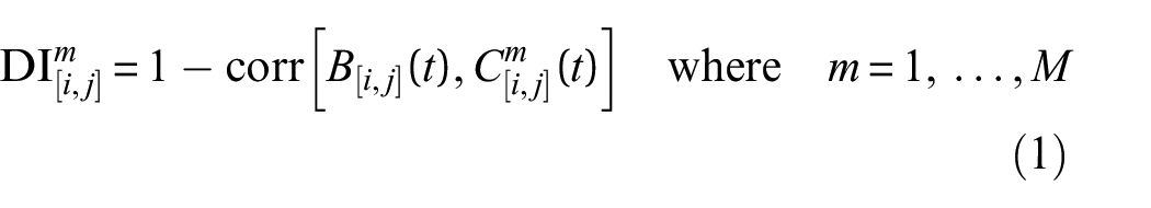
where
The damage index shown in equation (1) utilises the Pearson correlation coefficient. As a result, this damage index may sometimes not be a very robust statistical indicator for damage detection since it mainly captures non-linear attenuation, which occurs over long propagation paths. Therefore, linear attenuation, which occurs over short propagation paths, will not be captured relatively well. This damage index is used in this work because it has been demonstrated to work well for damage detection in large composite panels.16,17 The methodology presented in this current work is intended to be a framework for sensor path optimisation. Therefore, the user is free to change individual components of the methodology, such as the choice of damage index, based on their own preferences or applications.
During path optimisation, each sensor path in a network appears once. Due to signal reciprocity, a damage index will be computed, for example, for the path going from sensor 1 to sensor 2 and another for the path going from sensor 2 to sensor 1. Therefore, the average damage index for the paths between sensor
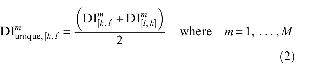
For example,
Let

where
and:
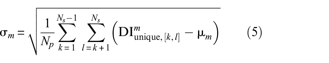
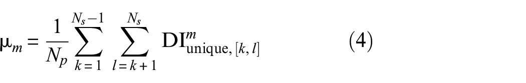
Given a reference dataset,
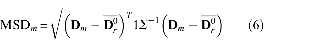
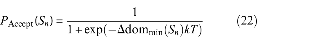
where
Equation (6), involves fitting a normal distribution to the reference dataset,
It is worth noting the variation of the guided wave signals with temperature can be very high. This will introduce large errors in the DI measurements in equation (1) which will influence the mean and variance matrices in equation (6). However, during the operation of SHM systems, there is often a great deal of variation/uncertainty regarding the temperature difference between baseline and current signals. Therefore, the presence of this variation in this work is intended to simulate typical operating conditions of SHM systems. Furthermore, the effect of temperature was compensated in the signals used, and only the residual of the compensation is included in the estimation of the mean and variance matrices.
Experiment details
In this work, a 1.624 × 0.94 m flat composite stiffened panel
16
was used for the collection of guided wave measurements. The frames of the panel are made of aluminium while the skin and the omega stiffeners are manufactured using carbon fibre reinforced polymer laminates of thermoset M21/194/34%/T800S unidirectional prepreg (Hexcel, GB). The stacking sequence of the composite is
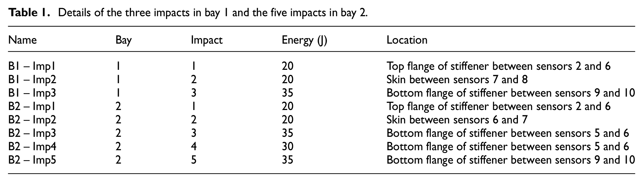
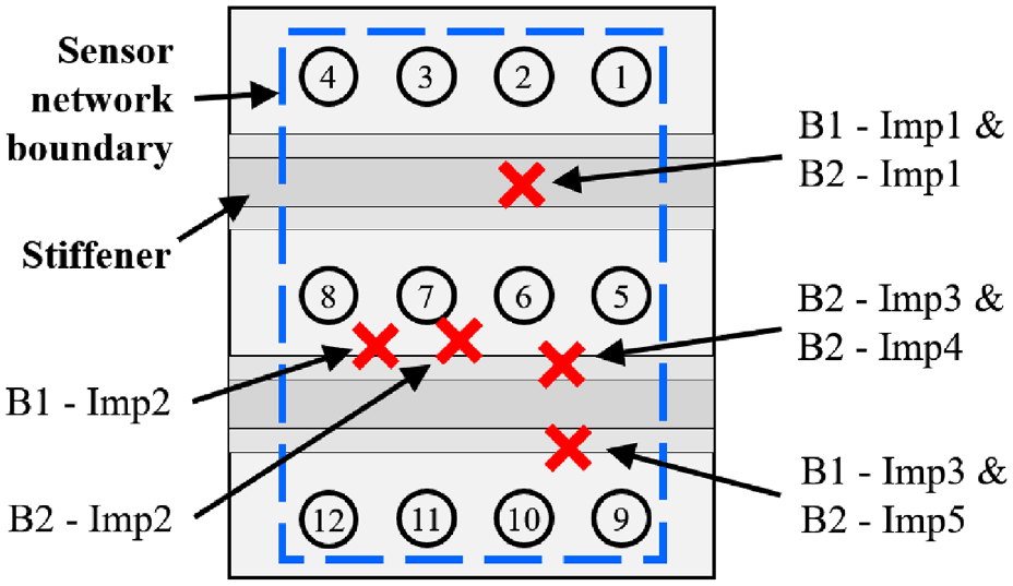
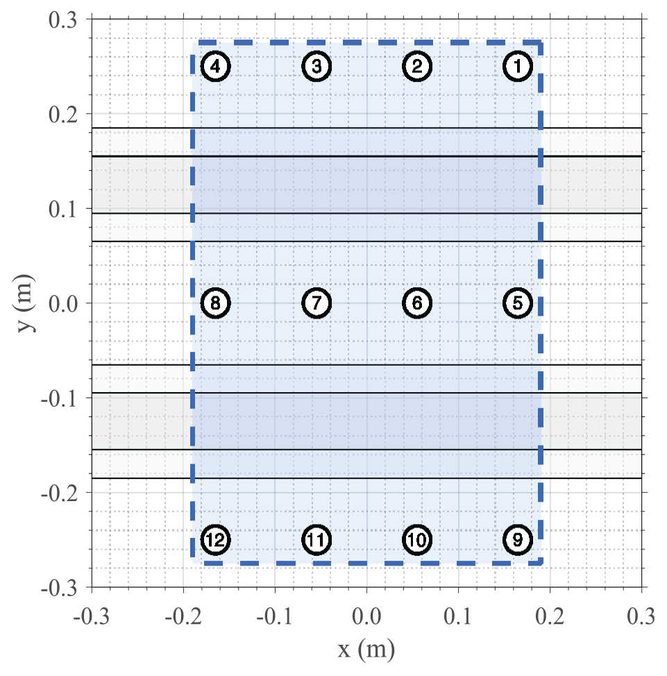
The central frame separates the panel into two bays. 12 DuraAct piezoceramic disks are surface mounted at each bay to monitor the health status of the panel. The panel geometry and sensor locations are illustrated in Figure 1. A National Instrument waveform generator and a PXI 5105 Oscilloscope (National Instruments, Austin, TX, USA) are used to actuate and sense the propagating guided waves. To evaluate the performance of the SHM system, guided wave measurements were recorded at both the pristine and damaged state of the structure. An INSTRON CREST 9350 drop tower (Instron, Norwood, MA, USA) with a 20 mm hemispherical impactor was used to impact the panel and introduce BVID. Since one of the objectives of this work is to optimise sensors paths to maximise the damage detection accuracy of an SHM network, the impact energy was selected to result in interlaminar delamination, undetectable via visual inspection. The presence and size of the BVID produced after each impact were confirmed using a portable C-scan device (Dolph Cam; Dolphitech, Gjøvik, Norway). Three identical panels were used, and a total of eight impacts were conducted, three in bay 1 and five in bay 2. Figures 1 and 2 show the flat panel used in this work. The locations of the impacts are shown, as well as C-scan images of the damage produced by the impacts. All impact events are summarised in Table 1. These impact energies were chosen as they are representative of a typical tool drop impact event.
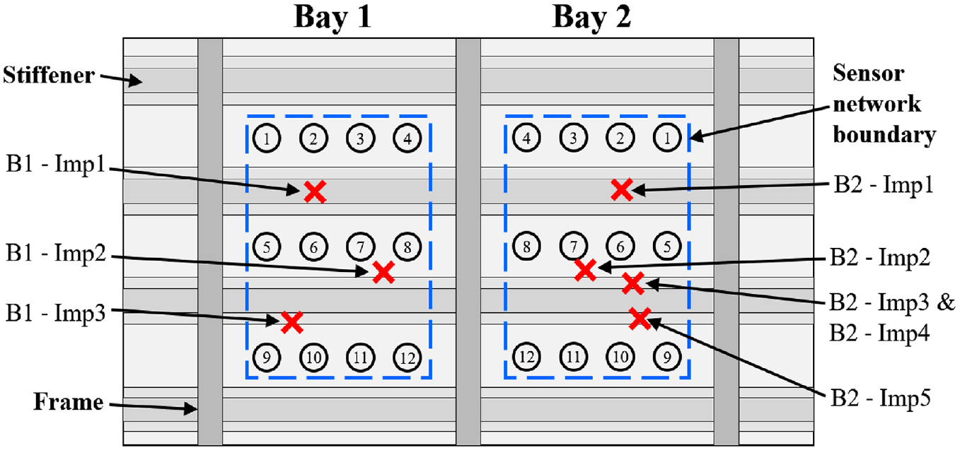
A diagram of the flat panel showing the locations of the bays, sensors, stiffeners, frames and impacts. The boundaries of the sensor networks are shown.
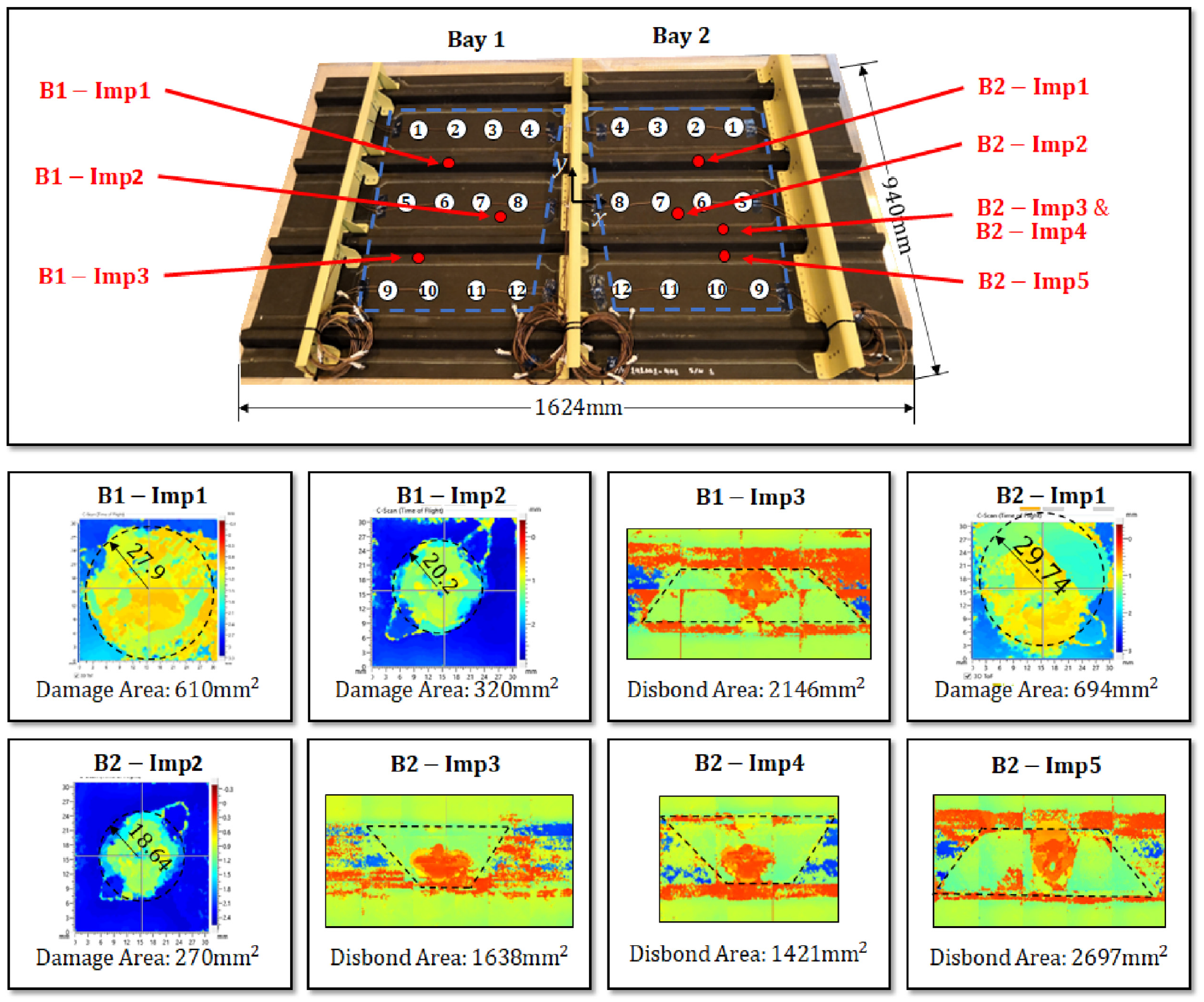
The flat panel used in this work. The locations of the impacts are shown, as well as C-scan images of the damage produced by the impacts.
Details of the three impacts in bay 1 and the five impacts in bay 2.
The actuation and sensing of guided waves is the specimen is carried out using surface-mounted DuraAct PZTs that are bonded using Hexcel Redux 312 adhesive film (Hexcel Corporation, Stamford, CT, USA). A chirp signal is used during excitation given as:
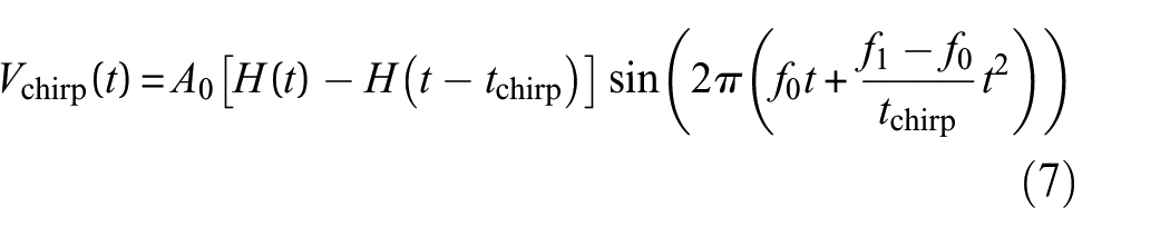
where
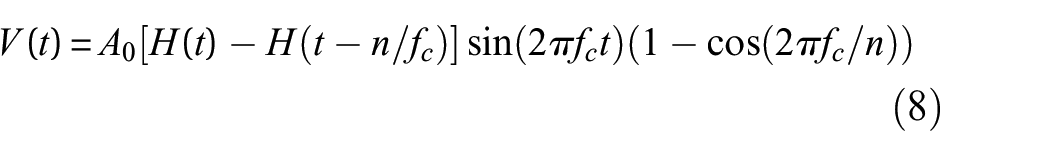
where n = 5 is the number of cycles in the tone burst and
A National Instrument waveform generator and a PXI 5105 Oscilloscope are used for data acquisition with a sampling frequency of
Regarding the measurements discussed in the second section, each measurement m consists of a complete interrogation of the sensor network where each PZT acts in turn as an actuator while the rest as sensors. Therefore, each measurement consists of a 12 × 12 matrix where each element of the matrix contains the signal recorded by a sensor pair. In total, 34 measurements were collected from all panels and temperature settings.
Since the two bays are identical in layout and symmetric about the central frame, bay 1 can be mirrored onto bay 2 to generate a superimposed approximation of the flat panel. As a result, the optimisation procedure can utilise the signal data from both bays, improving its reliability. This also means that the optimisation procedure only needs to be carried out on the superimposed approximation and not each bay individually. Once the optimal combination of sensor pairs is determined, this combination can be used directly with bay 2. However, it will need to be mirrored before it can be used with bay 1. The superimposed approximation of the flat panel is illustrated in Figure 3.
The superimposed approximation of the flat panel. Generated by mirroring bay 1 onto bay 2.
An extensive dataset of SHM measurements was collected from the flat panels. First, the panels were added to a climatic chamber, and measurements were collected for temperatures T = 25, 26, 30, 35, 40 and 45°C. The signals recorded at T = 25°C are considered the baseline signals
Sensor path network optimisation
If a sensor network contains
where

where
An example of a sensor path network consisting of four sensors. Five of the six possible sensor paths are used in the network.
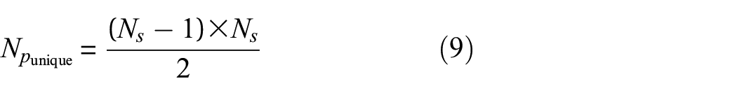
For a sensor network consisting of
For the panel studied here, as shown in Figure 3, there are 12 sensors, so
To reduce the computation time needed to investigate this large number of combinations, the optimisation procedure is split into two stages. In the first stage, the optimal paths connecting the 10 sensors on the network boundary are determined using simulated annealing (SA). This always results in 10 sensor paths being selected in the first stage. The purpose of this optimisation is to avoid large coverage gaps by ensuring that the paths along the boundary of the network are selected.
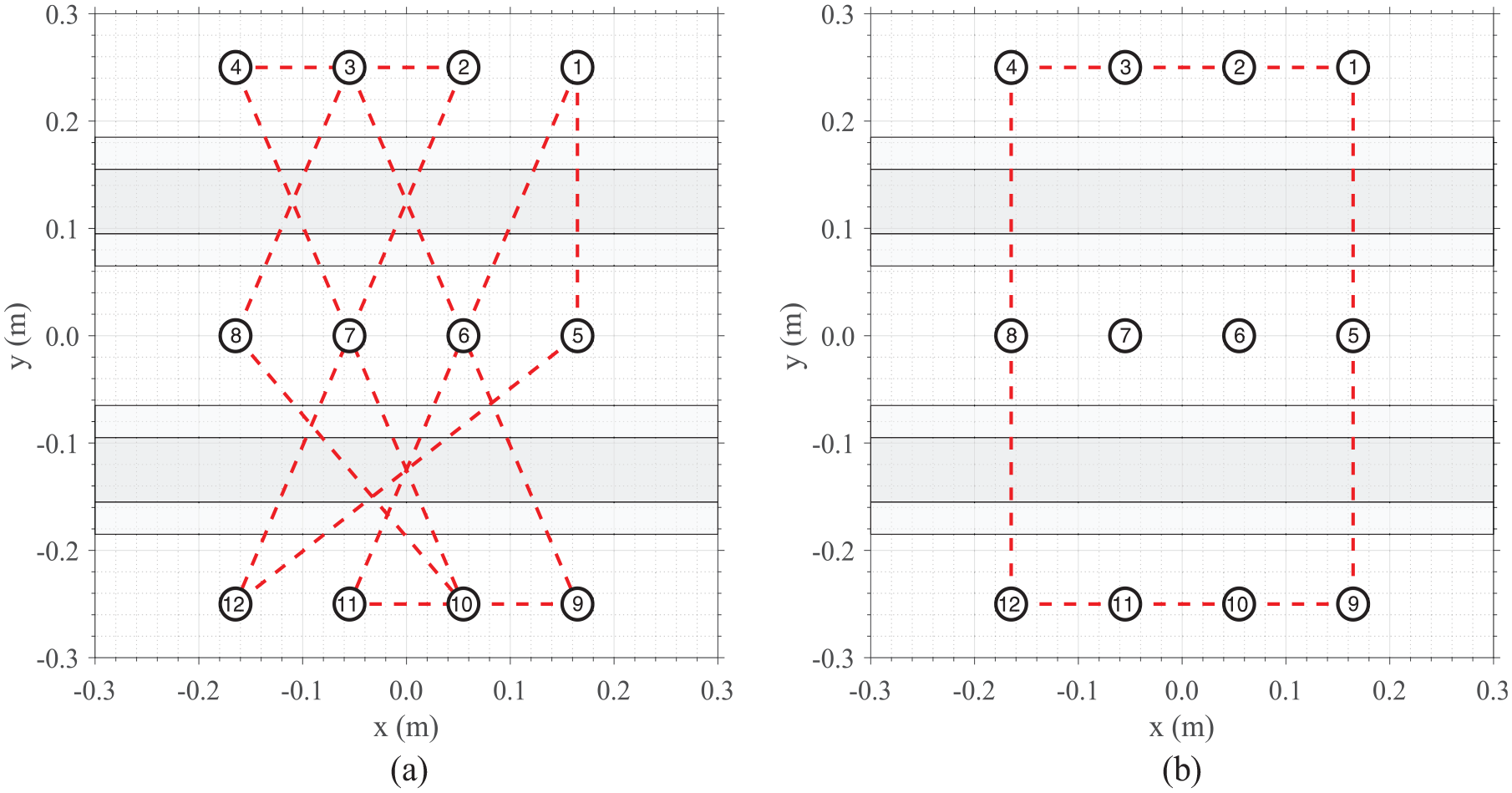
In the second stage, the optimal paths of the remaining 56 paths are then determined using a multi-objective form of SA known as AMOSA. 22 This means that up to 56 paths can be selected in the second stage. AMOSA is used to create a Pareto front balancing the three competing objectives described in the first section. To help visualise this, an example of an optimised network at the end of the first and second stages is shown in Figure 5.
A example of an optimised network at (a) the end of the first stage and (b) the end of the second stage.
By splitting the procedure into two stages, the number of possible unique sensor path combinations in the first stage is
Sensor path network optimisation: Boundary paths
In this section, the paths between the sensors on the boundary of the network are optimised using SA. Sensors on the interior of the network will be ignored in the optimisation procedure outlined in this section.
Simulated annealing
SA is probabilistic tool for global combinatorial optimisation problems that enables gradual convergence to a global near-optimal solution via a temperature cooling mechanism, analogous to the cooling used in the annealing technique in metallurgy to alter a material’s physical properties. 23
In each iteration, SA slightly perturbs the current solution
where

where
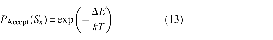
When a metal is heated to high temperatures in the annealing metallurgical technique, the metal’s atoms are highly mobile and become less mobile as the metal cools. This behaviour is replicated in SA via the temperature parameter T. It is clear from equation (13) that
In this work, the SA procedure was stopped when the new solution
Path optimisation
Ideally, when designing a sensor path network, the paths along the boundary of the network should be selected to avoid large gaps in sensor coverage. Also, as mentioned earlier, by determining the optimal boundary paths first, the efficiency of the overall optimisation procedure can be improved since the number of possible combinations to consider is reduced.
In this first optimisation stage, only the optimal paths between the boundary sensors are determined. For complex geometries or complex sensor layouts, it can be difficult for engineers unfamiliar with sensor networks to identify which sensors are on the boundary of the sensor network. To reduce the reliance of the proposed method on the experience of the user, the sensors on the boundary of the sensor network are automatically determined. Using the coordinates of the sensors, the convex hull of the sensor network can be calculated and is shown in Figure 6. This convex hull can be visualised as the shape enclosed by a rubber band stretched around the sensor network.
The convex hull of the sensor network.
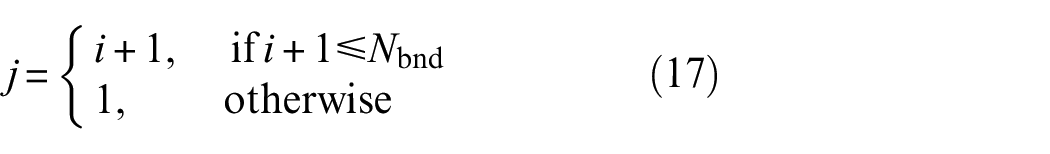
Sensors which lie coincident with the convex hull’s perimeter are identified as boundary sensors. These are sensors 1–12, excluding sensors 6 and 7. Before starting the SA optimisation procedure, a vector containing these sensors in a randomised order can be created:

The order in which the sensors appear in the vector
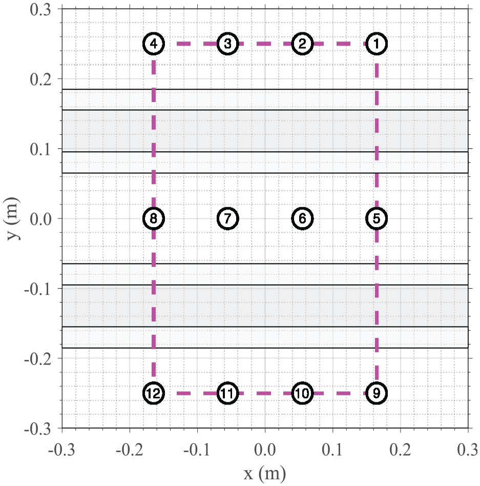
The sensor path network (a) before optimisation and (b) after optimisation.
When optimising the paths between the boundary sensors, the combination of sensors appearing in
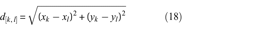
The total path distance,
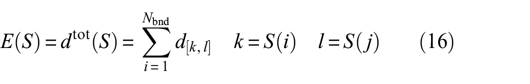
where
and
For example,
SA was used to determine the optimal paths between the boundary sensors to minimise
It can be seen in Figure 7 that the optimisation procedure significantly reduced the total path distance. The total path distance before the optimisation was

This optimal combination of sensor paths is shown in Figure 7.
Sensor path network optimisation: Remaining paths
As mentioned in the fourth section, there are a total of 66 unique sensor paths that can be selected in the network. In ‘Sensor path network optimisation: Boundary path’ section, 10 boundary paths were selected. Therefore, there are 56 remaining paths that need to be optimised. The goal of this optimisation procedure is to determine the optimal combination of remaining sensor paths to balance the three competing objectives described in the first section. All sensors 1–12 will be investigated in the optimisation procedure outlined in this section.
Since there are multiple objectives involved, the normal SA approach outlined in ‘Simulated annealing’ section cannot be used since it is for single-objective optimisation. Therefore, AMOSA, 22 a special form of SA for multi-objective optimisation is used in this work.
Archived multi-objective simulated annealing
The concept of Pareto-dominance is often found in multi-objective optimisation problems which involve competing objectives, whereby improving one objective can lead to a worsening of one or more other objectives. In these types of problems, if a solution provides worse outcomes for all of the objectives compared to other solutions, this solution is said to be Pareto-dominated. However, if a solution provides better outcomes for one or more objectives compared to other solutions, it is said to be Pareto-non-dominated or Pareto-optimal. AMOSA is a special form of SA for multi-objective optimisation. As the AMOSA algorithm progresses, it stores Pareto-optimal solutions in an archive. AMOSA incorporates the concept of Pareto-dominance using a parameter named domination. For a given number of objective functions
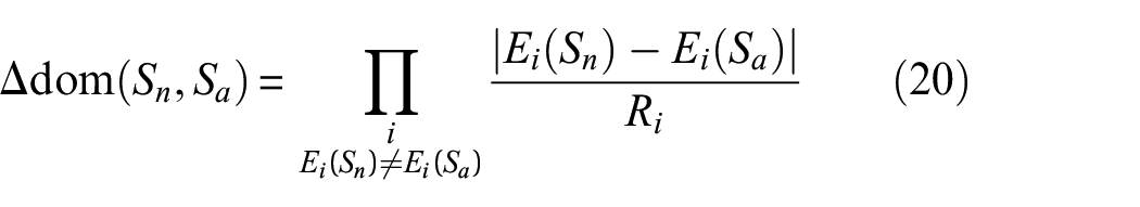
where
As in SA, in every iteration AMOSA slightly perturbs the current solution
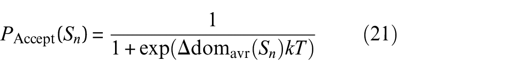
where
where
At the end of each iteration, the temperature parameter T is decreased according to a user-defined cooling scheme. The cooling scheme used in this work is:

where
In this work, AMOSA was stopped when the new solution
Path optimisation
For the path optimisation, AMOSA involves a number of objective functions
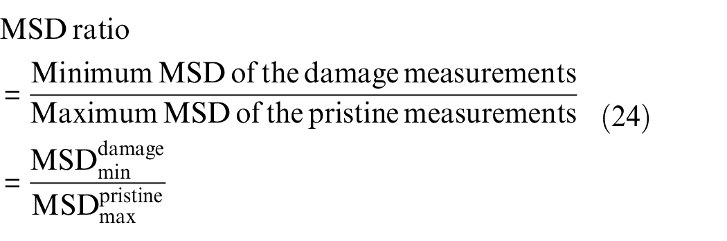
It is assumed that by maximising the MSD ratio in equation (24), the damage detection accuracy of the network is also maximised. This is because to maximise the MSD ratio, it is necessary to maximise
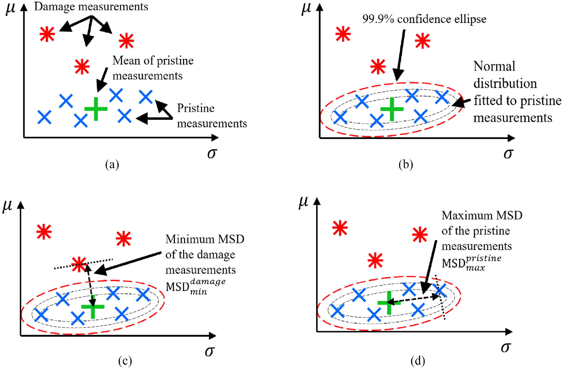
The four steps for calculating the MSD ratio. (a) Step 1: Plot the pristine and damage measurements. (b) Step 2: Fit a normal distribution to the pristine measurements. (c) Step 3: Calculate
In this work, the coverage area of a sensor path is calculated by drawing an ellipse between the two sensors of the path, as shown in Figure 9.
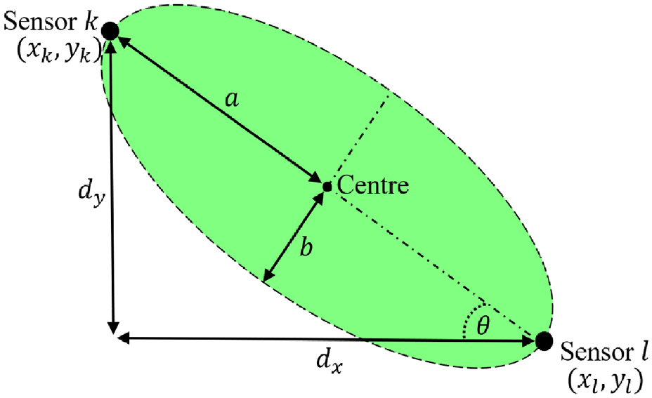
The coverage area of a sensor path between two sensors is determined using the area of an ellipse connecting the two sensors.
The semi-major axis a in Figure 9 can be expressed in terms of the distance
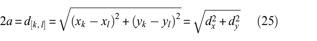
For a composite panel with the same thickness and material used in this work, it has been demonstrated that the typical diameter of a detectable BVID is around 5 cm. 16 Therefore, in this current work, the semi-minor axis b was given a fixed value of 2.5 cm, so that the width of the ellipse 2b is similar to the typical size of a detectable BVID.
The coverage area of the path between sensor k and sensor l shown in Figure 9 is:

The total coverage provided by the sensor paths of a network is calculated as a percentage of the area enclosed by the boundary of the sensor network:

where
The boundary of the sensor network.
From preliminary tests, there was no noticeable difference in total coverage area when the sensors were instead placed at the foci of the ellipse. Therefore, for simplicity, the sensors were placed at the ends of the ellipse in this work. If the sensors were instead placed at the foci of the ellipse, the methodology shown above would remain unchanged.
To determine the noise levels of each sensor path, the damage indices for the pristine measurements,
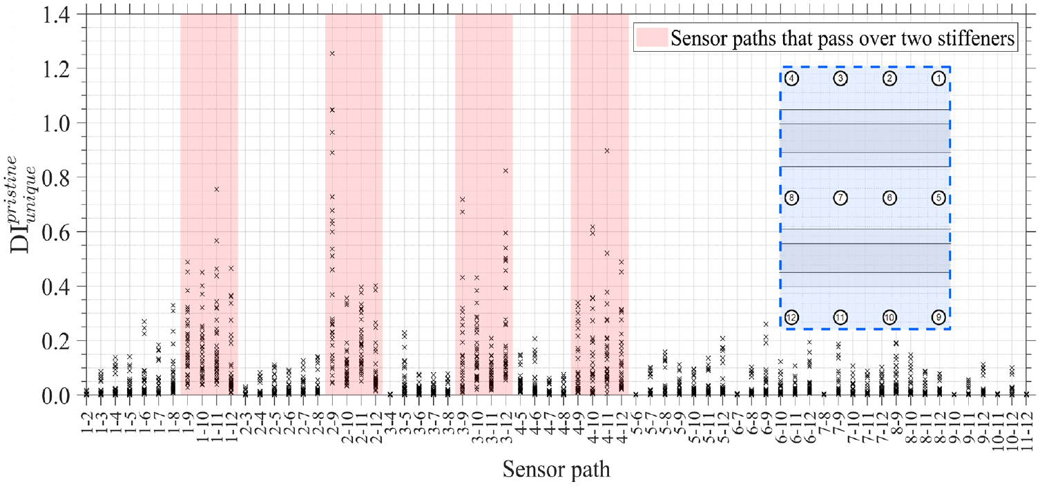
The damage indices of the pristine measurements. The paths that pass over two stiffeners are highlighted. The sensor network is shown on the right to aid comparisons.
It is clear from Figure 11 that there is a much larger spread in
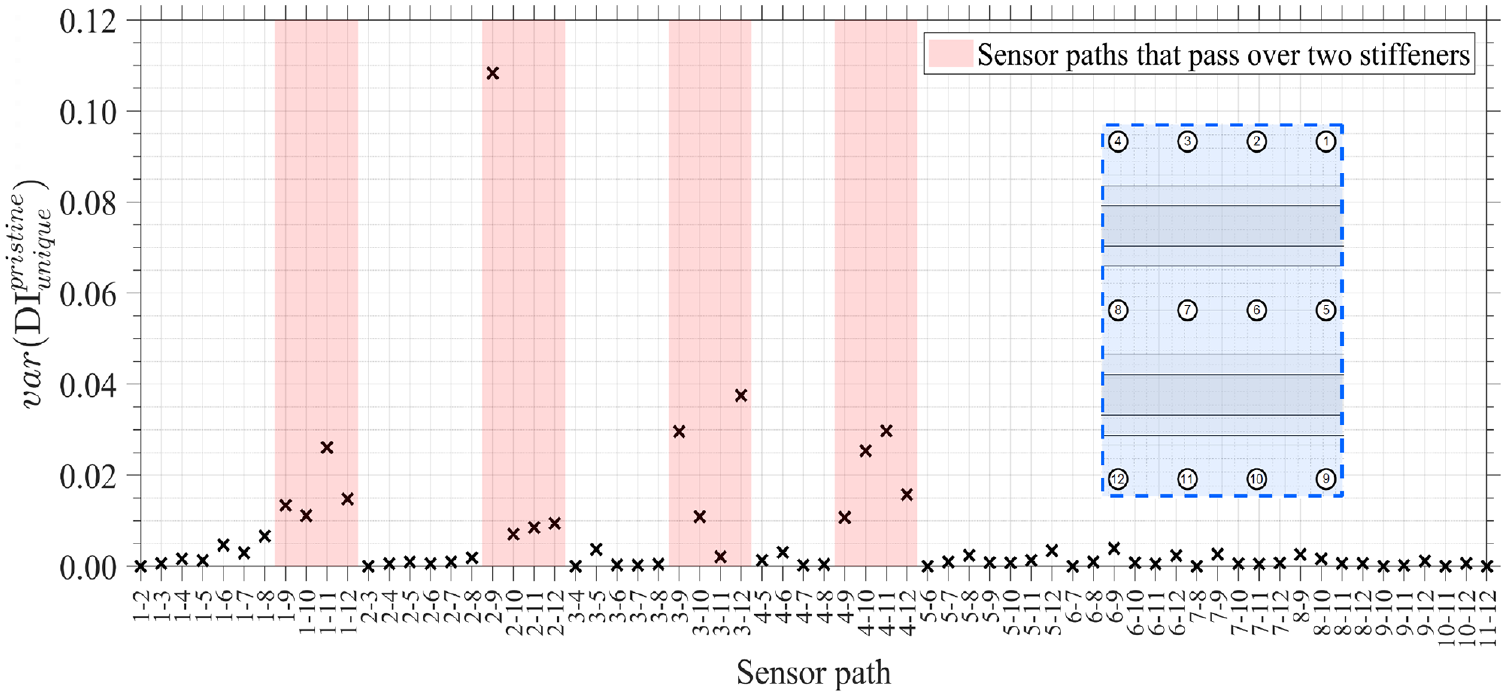
The variance of the damage indices of the pristine measurements. The paths that pass over two stiffeners are highlighted. The sensor network is shown on the right to aid comparisons.
It can be seen in Figure 12 that the paths that cross over both stiffeners give the highest variance in
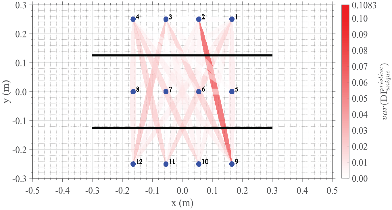
Damage index variance map for the entire sensor network.
The damage index variance map in Figure 13 makes it clear that longer paths and paths that pass over both stiffeners demonstrate much higher variances in their damage indices. As a result, there is a great deal of noise in the pristine damage indices of these paths, making them less reliable for damage detection. Therefore, when optimising the damage detection accuracy of the network, sensor paths with high variance in
Results and discussion
As mentioned in ‘Sensor path network optimisation: Remaining paths’ section, the three objective functions used in AMOSA were:
1. To maximise the damage detection accuracy of the sensor network. This corresponds to maximising the MSD ratio introduced in ‘Sensor path network optimisation: Remaining paths’section.
2. To maximise the sensor coverage area of the sensor network.
3. To minimise the overall noise present in the sensor network.
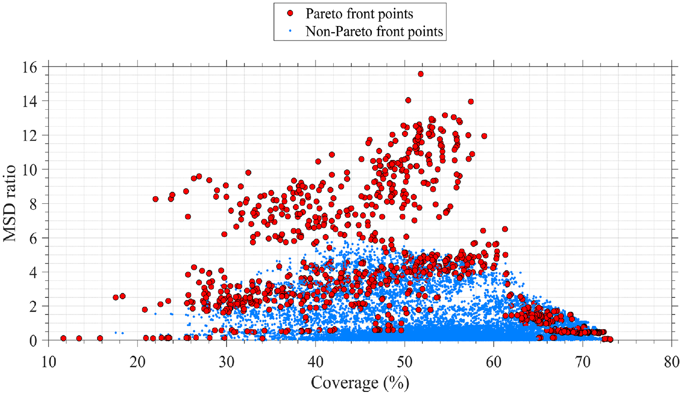
The results obtained from AMOSA for these three objective functions can be seen in Figure 14. Side views of Figure 14 can be seen in Figures 15 to 17. A total of 10,000 AMOSA iterations were completed, producing 10,000 solutions. Of these, 1148 were non-dominated solutions, also known as Pareto front solutions, and 8852 were dominated solutions, also known as non-Pareto front solutions. These solutions are shown as red and blue markers, respectively, in Figure 14.
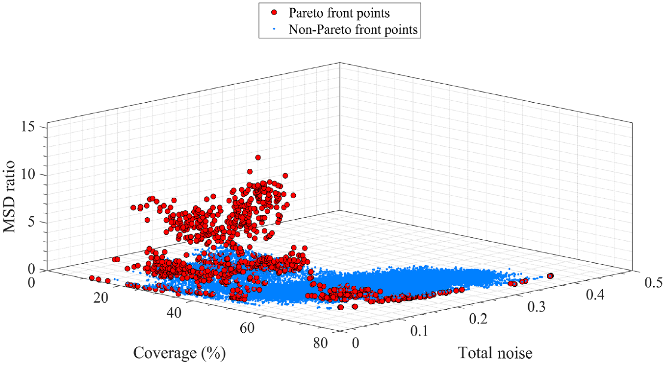
Results from the multi-objective sensor path optimisation using AMOSA.
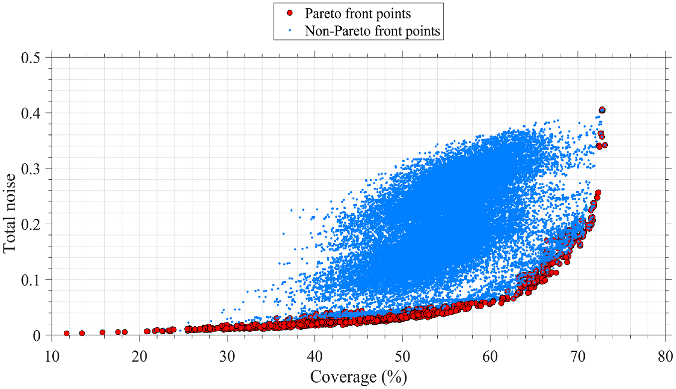
Results from the multi-objective sensor path optimisation using AMOSA. Side view of Figure 14, Total noise versus coverage.
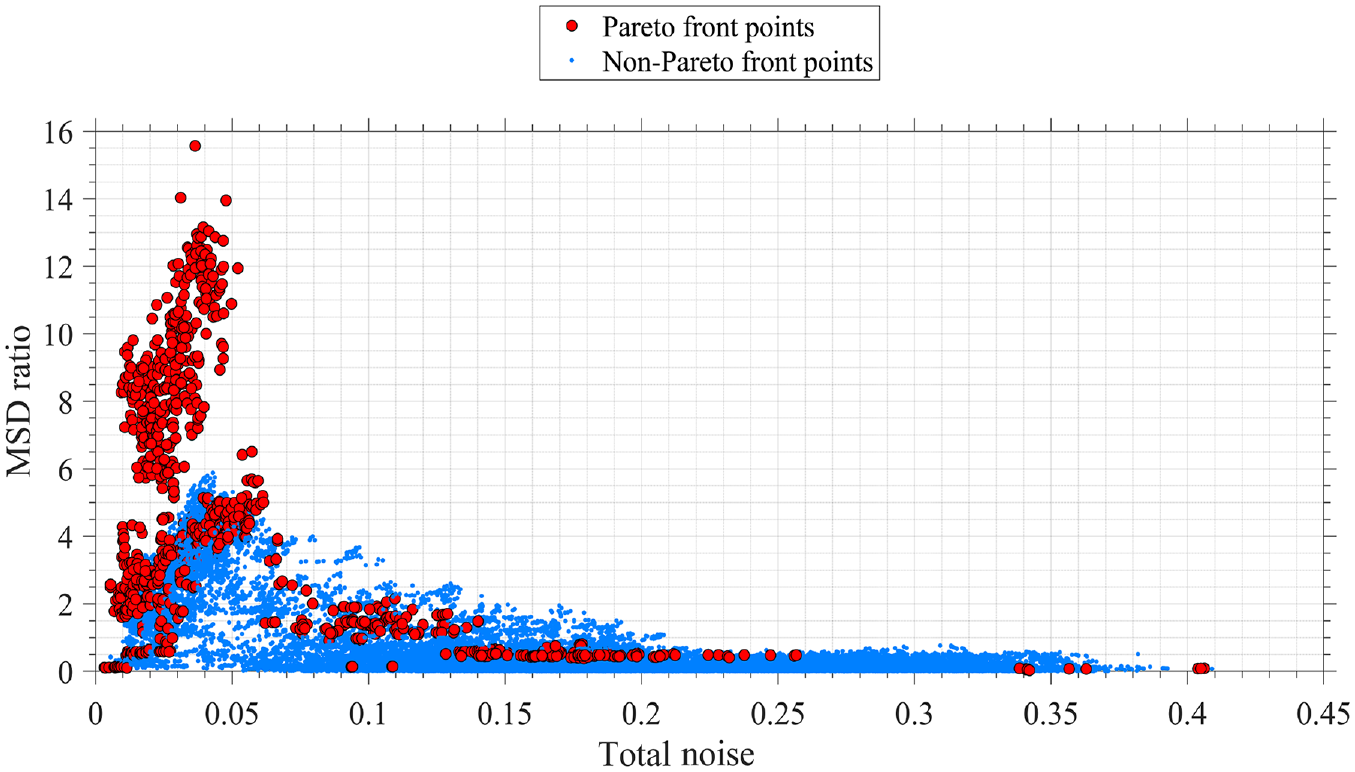
Results from the multi-objective sensor path optimisation using AMOSA. Side view of Figure 14, MSD ratio versus total noise.
Results from the multi-objective sensor path optimisation using AMOSA. Side view of Figure 14, MSD ratio versus coverage.
In Figure 15, it is clear that as the coverage level increases, the total noise also increases. This is due to the fact that longer sensor paths contribute more to the coverage level but also significantly increase total noise, as found in ‘Path optimisation’ section.
Figure 16 shows that the damage detection accuracy, in the form of the MSD ratio, decreases as the total noise increases. This is because an increase in total noise leads to a wider spread of the pristine and damage measurements, therefore increasing
It can be seen in Figure 17 that for coverage levels below 60%, there is no clear relationship between the MSD ratio and the coverage level. However, once the coverage level is above 60%, it is clear that the MSD ratio decreases as coverage level increases. This is due to the fact that higher coverage levels are strongly associated with higher values of total noise, as shown in Figure 15, thereby reducing damage detection accuracy.
Given that there are 1148 Pareto front solutions in Figure 14, it can be difficult to choose a suitable solution. To simplify the process of choosing a suitable solution, the engineer can apply a filter to these solutions by defining suitable ranges for the objective functions. For example, the engineer could define
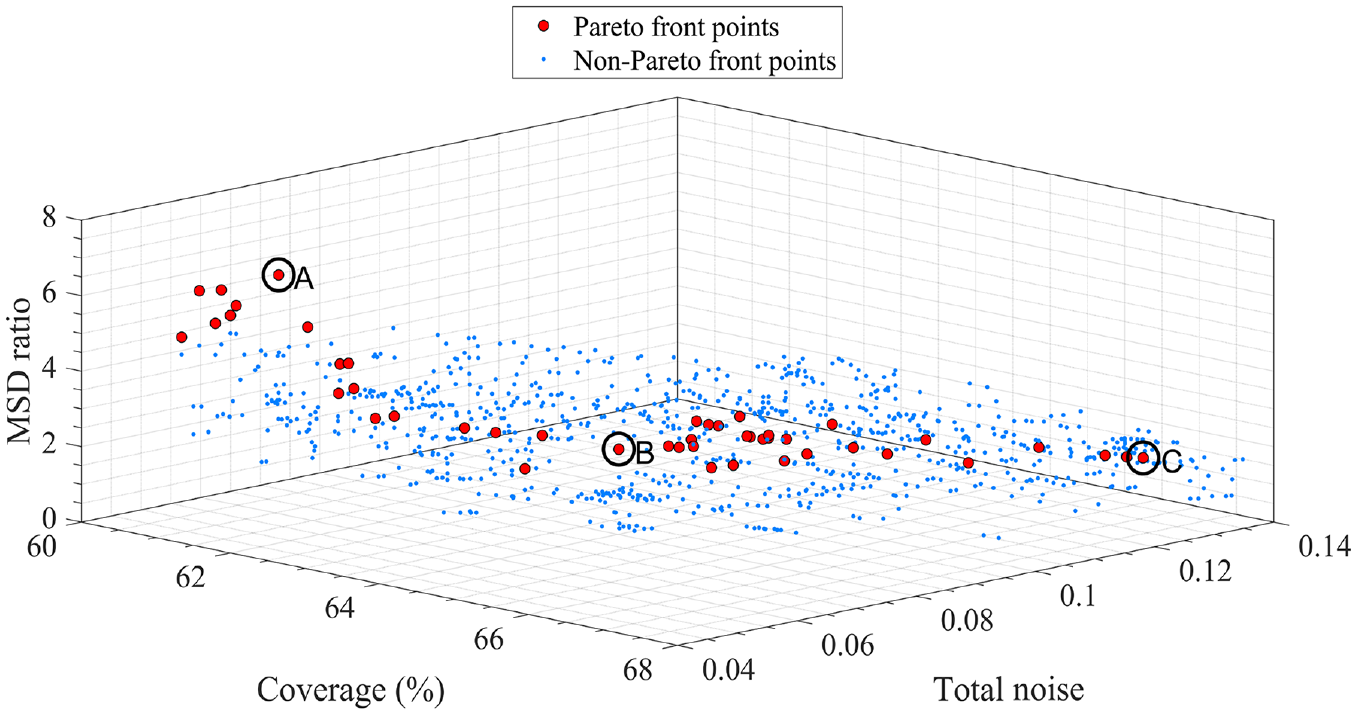
Pareto front solutions obtained for the case where the coverage level is above 60% and the MSD ratio is greater than 1.5. Three potentially suitable Pareto front solutions have been highlighted by blue circles and labelled ‘A’, ‘B’ and ‘C’.
All three objectives (MSD, coverage and total noise) should be considered when choosing a solution. The values of the coverage, MSD ratio, and total noise for these three solutions can be seen in Table 2 for solutions ‘A’, ‘B’ and ‘C’. The coverage maps for solutions ‘A’, ‘B’ and ‘C’ are shown in Figure 19. The means and standard deviations of the damage indices for the pristine and damage measurements for solutions ‘A’, ‘B’ and ‘C’ are shown in Figure 20. To see how well solutions ‘A’, ‘B’ and ‘C’ perform against the case where all of the sensor paths are used and the case where prior expert knowledge is used to select the sensor paths, the results for these two cases are given in Table 2, Figure 19 and Figure 20. For the case of prior expert knowledge, the sensor paths selected by Yue et al. 16 were used.
Values of the objectives for solutions ‘A’, ‘B’, ‘C’ and the case where all sensor paths are used.
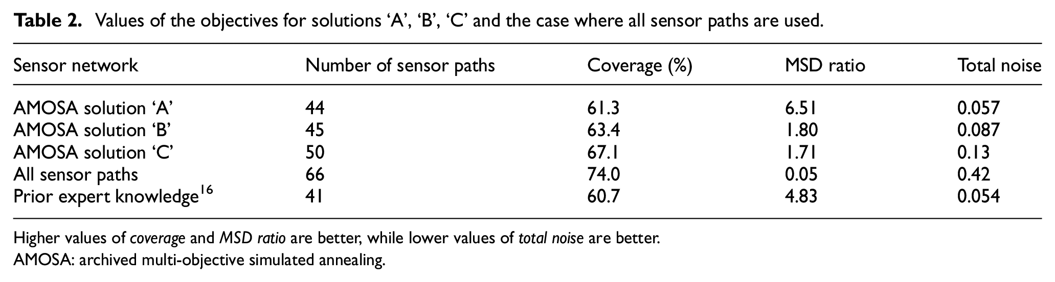
Higher values of coverage and MSD ratio are better, while lower values of total noise are better.
AMOSA: archived multi-objective simulated annealing.
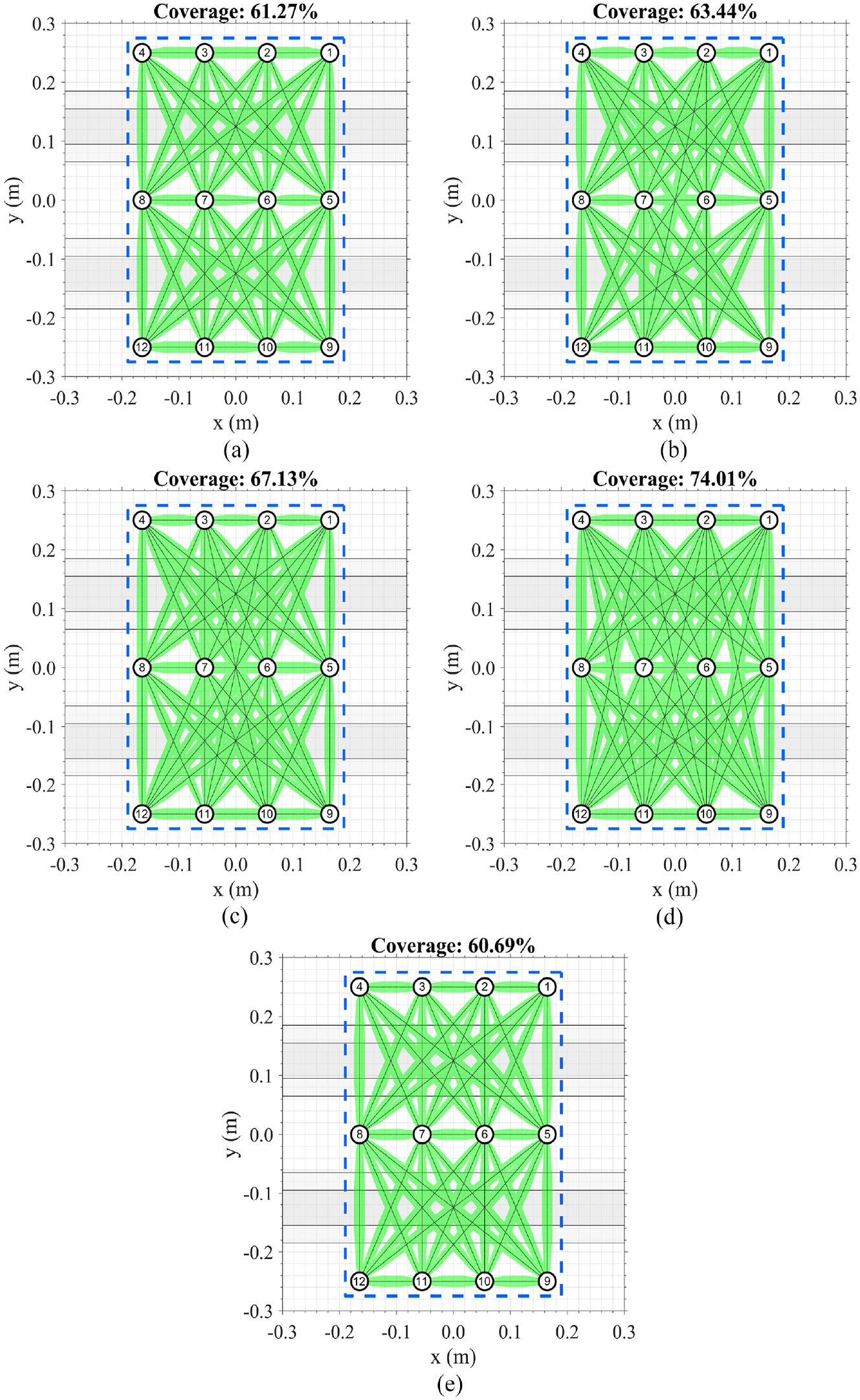
Coverage maps for different sensor networks. The network boundary is shown as a dashed blue line. (a) Solution ‘A’. (b) Solution ‘B’. (c) Solution ‘C’. (d) All sensor paths. (e) Prior expert knowledge. 16
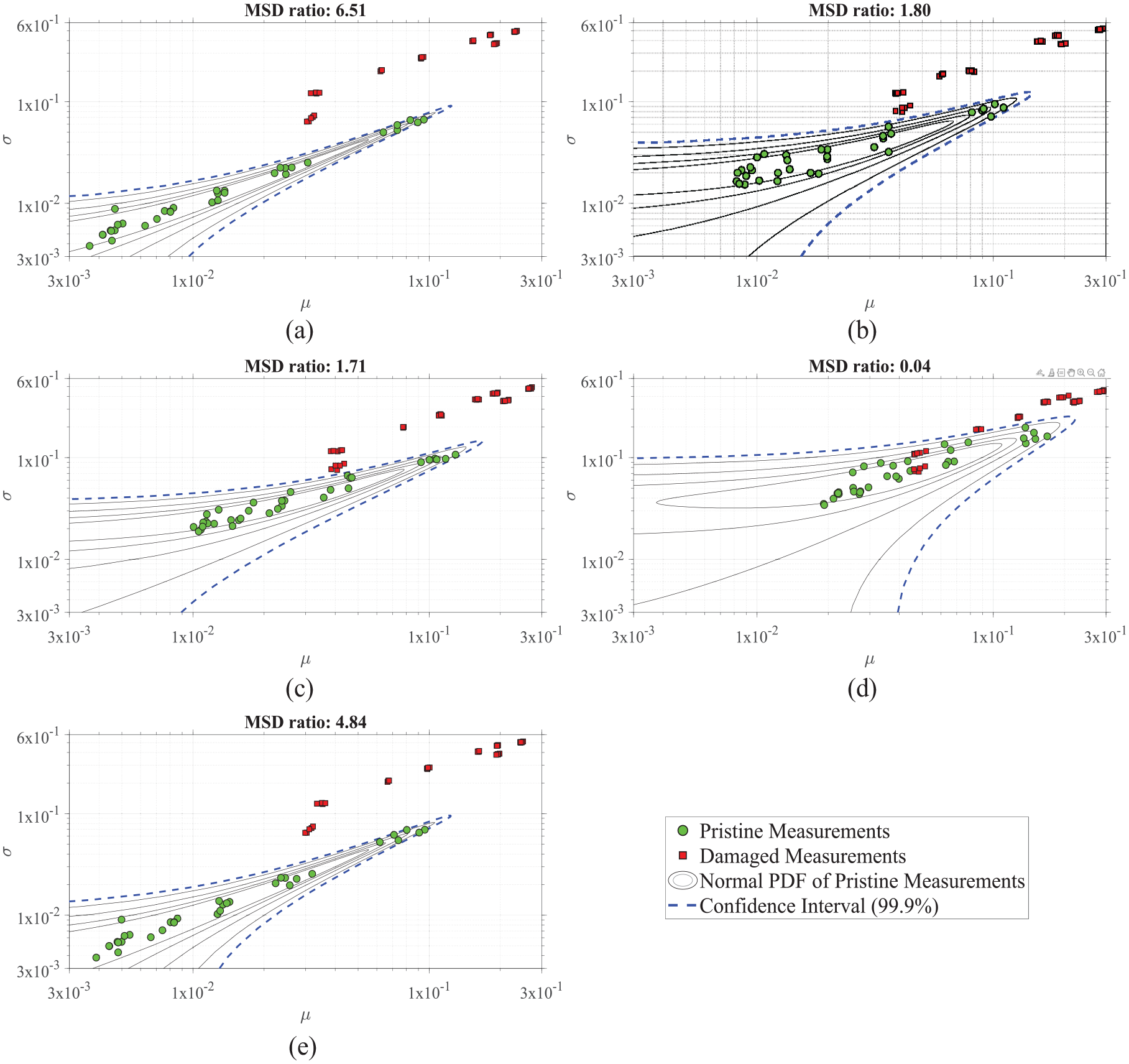
Means and standard deviations of the damage indices for the pristine and damage measurements for different sensor networks. (a) Solution ‘A’. (b) Solution ‘B’. (c) Solution ‘C’. (d) All sensor paths. (e) Prior expert knowledge. 16
As shown in Figure 19, solution ‘A’ and solution ‘C’ provide the lowest and highest coverage levels, respectively, among the AMOSA solutions considered. The coverage levels for solution ‘A’ and the solution with prior expert knowledge are very similar, but there are some slight differences - unlike the solution where prior expert knowledge is used, solution ‘A’ uses paths 1–3, 2–4, 6–8 and 10–12, while it doesn’t use path 6–7. The inclusion or exclusion of these paths does not cause much difference in coverage but has a significant impact on the MSD ratio, as seen in Table 2.
As expected, the solution involving all of the sensor paths provides the highest coverage level since it utilises the sensor paths that cross over both stiffeners. Solution ‘A’ does not use any sensor paths crossing two stiffeners, while solutions ‘B’ and ‘C’ utilise four and seven, respectively. These paths provide the largest increase in coverage level among all of the paths, but they also provide the largest increase in total noise, which reduces damage detection accuracy, as represented by the MSD ratio. This is clearly seen in the data presented in Table 2, where solution ‘A’ provides the highest MSD ratio and lowest total noise. Compared to the case where prior expert knowledge is used to select the sensor paths, solution ‘A’ provides a very similar coverage level (61.3 vs 60.7 %) and total noise (0.057 vs 0.054).
The lower total noise from the solution with prior expert knowledge could be because the performance index total noise is being used in this work and not average noise. Therefore, as the number of paths in a network increases, the total noise also increases. As a result, a network with less paths can demonstrate a lower total noise. Since the solution with prior expert knowledge has a low number of paths compared to the other solutions investigated, it follows that it would also have a low total noise.
The impact on damage identification accuracy from utilising more sensor paths that cross over both stiffeners is most clearly depicted in Figure 20. It can be seen in this Figure that it becomes progressively more difficult to distinguish the damaged measurements from the pristine measurements as more sensor paths crossing over both stiffeners are used. This is represented by the MSD ratio, which drops sharply from 6.51 for solution ‘A’, to 0.04 for the solution where all of the sensor paths are used.
Solution ‘A’ provides similar performance, in terms of coverage and total noise, to the other solutions. However, it also provides significantly higher damage detection accuracy than the solution where prior expert knowledge is used – solution ‘A’ gives an MSD ratio of 6.51 compared to an MSD ratio of 4.83 for the solution where prior expert knowledge is used, an increase of 35%. This difference can be seen visually in Figure 20– there is less spread in the pristine measurements in Figure 20(a) compared with Figure 20(e). The confidence interval envelope in Figure 20(a) is also more narrow than in Figure 20(e). This difference could be because solution ‘A’ uses a slightly different network of paths compared to the solution where prior expert knowledge is used. Unlike the solution where prior expert knowledge is used, solution ‘A’ uses paths 1–3, 2–4, 6–8 and 10–12, while it doesn’t use paths 6–7. Paths such as 1–3, 2–4, 6–8 and 10–12 are not typically considered in SHM networks since if a network contains paths 1–2, 2–3 and 3–4, then adding path 1–3 or 2–4 will not noticeably improve the coverage of the network. 16 However, based on the high MSD ratio of solution ‘A’, the addition of these paths could significantly improve damage detection and the overall performance of the SHM network.
In this work, paths that pass over both stiffeners demonstrated much higher noise than paths that only cross one stiffener. Therefore, paths that pass over both stiffeners are more likely to be removed. This can most clearly be seen by solution A from AMOSA in Table 2, which didn’t use any paths that cross both stiffeners. The removal of these paths is also seen in the solution based on prior expert knowledge. 16 In this solution, paths that pass over two stiffeners were not used, but good localisation performance was demonstrated.
A potential improvement to the methodology shown in this work would be to include an objective describing the localisation performance of the network. This objective could be based on probability of detection or probability of localisation.
Conclusions
This work proposed a novel methodology for the automatic multi-objective optimisation of sensor paths in a SHM sensor network using SA. Using all of the sensor paths within a sensor network may not always improve the performance of the network. In fact, the removal of some paths may even improve the overall performance of a SHM sensor network. For example, the results obtained in this study indicate that the removal of paths that demonstrate a high level of overlap with other paths or paths that cross multiple structural features (e.g. stiffeners) can improve multiple objectives. The former do not provide any additional information, while the latter contain significant noise that affects the detection accuracy of the SHM system. Removing these paths leads also to a reduction in the complexity of the network.
Knowing which paths to include, and which to exclude, can require significant prior expert knowledge, especially in the case of structures with complex geometries. Furthermore, paths selected on the basis of the engineer’s expertise and knowledge do not necessarily provide an optimal solution, as such an optimal solution should take into account different and complex performance measures. Therefore, the automatic multi-objective optimisation procedure developed in this work aims to select the paths of an SHM sensor network that maximise coverage level, maximise damage detection accuracy, and minimise signal noise due to the presence of geometric features, with minimal user intervention.
Furthermore, a significant benefit of the proposed optimisation procedure is that it is scalable to different structures of varying complexity and can be used with panels of any material and with any UGW damage detection methodology. The proposed procedure does not change based on the details of the damage detection methodology, but the objectives used in the procedure should be based on UGW principles for damage detection.
The proposed procedure was tested on a real-world large composite stiffened panel, with many geometric features in the form of frames and stiffeners. 16 The panel was subjected to impact damage from eight impact events. A Pareto front was created using a multi-objective form of SA known as AMOSA to balance the three competing objectives. Compared to selecting all possible paths, the optimised sensor paths achieve higher damage detection accuracy and lower signal noise, although the coverage is slightly lower. Compared to the case where expert knowledge was used to select the sensor paths, the proposed optimisation procedure provided a similar coverage level and total noise but gave 35% higher damage detection accuracy. These results demonstrate that the novel automatic optimisation procedure proposed in this work is capable of providing a sensor path network whose performance is superior or equal to the performance of sensor path networks designed using prior expert knowledge, with minimal user input.
Footnotes
Declaration of conflicting interests
The author(s) declared no potential conflicts of interest with respect to the research, authorship, and/or publication of this article.
Funding
The author(s) disclosed receipt of the following financial support for the research, authorship, and/or publication of this article: The research leading to these results has gratefully received funding from the European JTICleanSky2 program under the Grant Agreement n° 314768 (SHERLOC). This project is coordinated by Imperial College London.