
Abstract
This paper presents a practical and efficient workflow for deformation monitoring of transport infrastructure. We propose using commercially available mobile laser scanning (MLS) systems to scan civil infrastructure while driving by in a car or rail vehicle. Our processing pipeline corrects for MLS-specific systematic deviations and models deformations from point clouds of two epochs. Following the concept of rigorous deformation analysis, we statistically test the deformations for significance. The required point cloud uncertainty may be obtained in two ways. First option is empirically by multiple passes and, secondly, by prediction with a learned stochastic model. We apply the method to three retaining structures and evaluate results based on ground truth geodetic surveys. The deviations did not exceed 10 mm, even for complex object surfaces or when traveling at 80 km/h. We demonstrate that the method is capable of revealing displacements in the centimeter range without relying on any installations on the structure. The approach shows great potential as a novel, efficient tool for detecting and quantifying defective structures in a road and railway network.
Keywords
Introduction
Structural Health Monitoring (SHM) aims to observe a structure through measurements, extract damage-related parameters, and analyze data to assess the current state of health. 1 Depending on the structure or mechanical system, different damage-sensitive features may be relevant for monitoring. In transport infrastructure maintenance, geometry is a frequently monitored parameter for bridges, tunnels, roads, rails, and retaining walls. 2 The term deformation monitoring refers to the process of observing structural geometry changes, that is, strain, bending, torsion, displacement, and rotation. 3
Geodetic monitoring established itself as a versatile solution for safety-critical applications.4,5 It includes optical surveys with total stations to distinct points mounted on the structure of interest and of stable points placed outside the deformation area. The processed angle and distance measurements provide 3D coordinates of these points in the established reference coordinate frame. A notable advantage of optical surveys with total stations is that by observing the same points from multiple setup locations, it is possible to assess the reliability and quality of the results. Consequently, the engineer can decide whether displacements of the points are significant or within the measurement uncertainty. The term rigorous deformation analysis stands representative of this approach.
Another related technology that has become increasingly popular for monitoring recently is terrestrial laser scanning (TLS). Many aspects are identical to traditional geodetic monitoring, including the measurement parameters and the establishment of a stable coordinate frame by reference points with known and stable coordinates. The main difference is that terrestrial laser scanner sample the entire structural surface in angular increments. The resulting point clouds provide rich geometry information. In contrast to total station monitoring, there are no point correspondences in laser scans acquired at different times, though. Due to the irregular object sampling by TLS, a direct comparison of 3D coordinates is thus not possible. So different strategies have evolved to derive information about geometry changes from point clouds. Some are very flexible and applicable to almost any object while others are designed for specific-use cases but require a high degree of manual interaction. Another side effect of no point being measured twice is that no information about quality or reliability can be derived, as is the case with total station measurements. This fact raises the question of how to carry out rigorous deformation analysis if no uncertainty information is available for the point clouds. So far, no standard operating procedure is available, and research is still ongoing.
In recent years, new mobile laser scanning (MLS) devices came onto the market, promising increased productivity. The workflow differs greatly from TLS as point clouds are captured while moving around with a backpack and handheld devices, remotely steering drones and robots or operating systems on land-based vehicles. In particular, MLS systems mounted on a car or railway vehicle seem promising for infrastructure monitoring (see Figure 1). Collecting data without impeding traffic flow or closing lanes brings huge cost and time benefits.
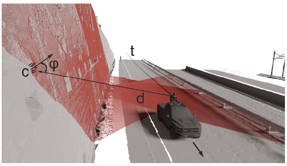
Concept of deformation monitoring using mobile laser scanning and the quality influencing factors: trajectory (t), distance (d), angle of incidence (
Despite the clear advantages, there are few to no case studies in which this relatively young and expensive measurement technology is used for such safety-critical applications. In other words, there is a lack of practical experience. In this publication, we summarize the key findings from 6 years of experience surveying 24 retaining structures with four commercial MLS systems and processing 300-point clouds with approximately 7 billion points.
In this paper, we focus on three retaining structures A, B, and C (see Figure 2). The selection of structure A is motivated by the fact that extensive reference data with total stations and high-frequency tilt values with a low-cost wireless sensor system is available for more than 1 year. B represents a typical retaining structure with ongoing geodetic monitoring by a service provider and C is a structure where large deformations have actually occurred due to nearby construction works.
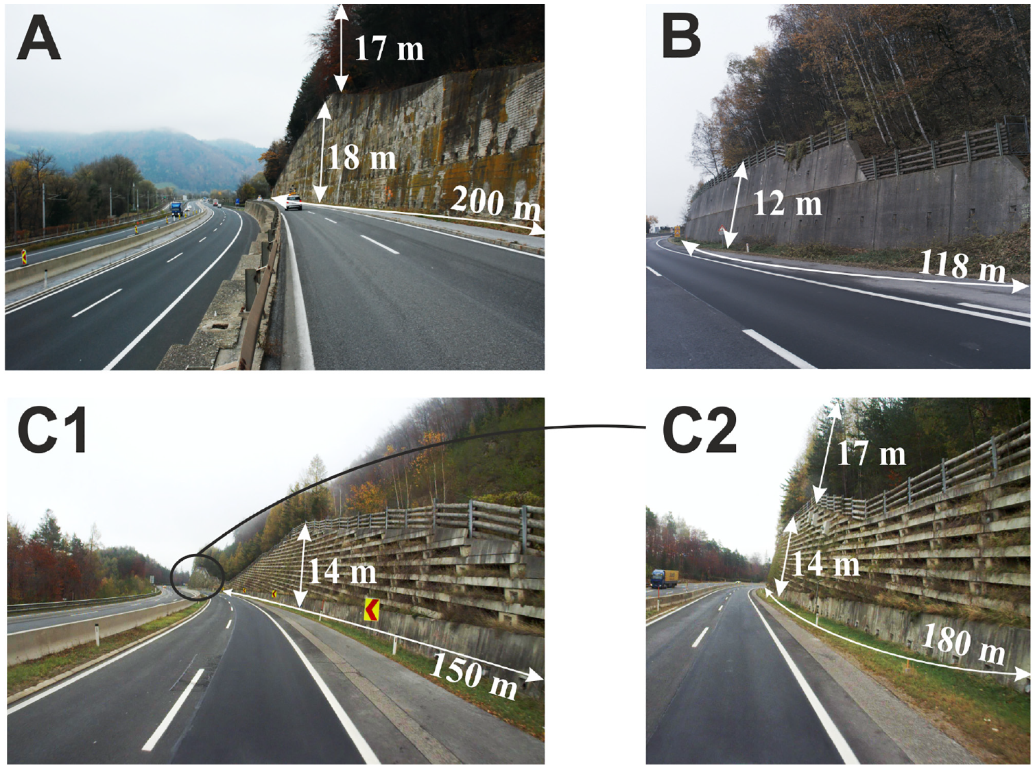
Three retaining structures A, B, C serve as examples for the proposed workflow in this paper. The illustrations also show the structural dimensions and the extent of vegetation growing above the objects.
Our aim is to achieve a workflow that provides reliable data on deformation and uncertainty using MLS (see Figure 1). The proven rigorous deformation analysis of point-wise displacements by total stations presents the benchmark for the new method. This paper elaborates the individual components of the workflow, focusing on the following challenges:
Objects of transport infrastructure vary in shape and size. A deformation modeling strategy for point clouds should thus be flexible and highly automated for large-scale application.
The uncertainty of the results depends on data acquisition and processing and is unknown a priori. However, knowledge about precision and accuracy is crucial to obtain trustworthy results and to distinguish between significant deformations and measurement uncertainty.
MLS enables fast data collection but the question remains of how to establish a stable reference frame efficiently. The old-proven method of measuring reference points with total stations proves too time-consuming and thus costly.
This article first introduces the reader to the concept of rigorous deformation analysis of total station measurements, applications of TLS, and the challenges associated with using MLS. Building on existing work, we then provide details of our tailored workflow to address the challenges identified above. Finally, we present the results and evaluate them using geodetic monitoring data for the three retaining structures A, B, and C (see Figure 2).
State-of-the-art in laser scanning and deformation monitoring
Rigorous deformation analysis of total station measurements
Total stations are optical surveying instruments that measure horizontal, vertical angles, and distances
Optical surveys provide empirical uncertainty information for the 3D coordinates when carried out from multiple setup stations (see Figure 3, left). From a statistical point of view, this procedure is equivalent to drawing multiple samples independently from a population. Hence, faulty observations are detectable mathematically and results are more trustworthy. The typical processing procedure establishes an over-determined, linear equation system
Rigorous deformation analysis geodetic surveys at retaining wall A: schematic representation of observing distinct points on the structure from three setup stations (white, black, and red lines; left); horizontal displacement vectors and 95% confidence ellipses (right); red ellipses indicate significant deformations while the green ones represent stable points.
Geodetic monitoring has been around for decades and much experience has been built up regarding its performance and the accuracy of the calculated displacement vectors. Knowing the quality of the measurement data is crucial to obtaining trustworthy and interpretable results and ultimately adding value to the assessment of the health condition of a structure.
Reference frame for laser scanning point clouds
Like total stations, laser scanners record angle and distance measurements, but with the big difference of sampling the entire object surface instead of selectively measuring individual points.
Another similarity to total station measurements is that a reference frame is also needed to register the local point coordinates of each scan. There are two approaches to realizing the reference frame. The first involves installing reference points and determining their coordinates by performing optical surveys with total stations in advance. The prism targets are then replaced by circular or flat targets that are recognizable in the laser scans. Representative case studies use this registration method for monitoring of dams,11,12 lock gates, 13 bridge decks, 14 and television towers. 15 The second method relies on computing transformation parameters between scans by minimizing discrepancies for stable reference surfaces. This method is preferable if reference points are very close to the setup station or do not exist at all. Such a situation is typical for rockface or landslide monitoring. The challenge is finding reference surfaces, especially for data sets that were collected with a large time gap. There are multiple publications following similar strategy . First, the point cloud is subdivided using an octree data structure before computing centroid displacements 16 or applying the Iterative-Closest-Point (ICP) algorithm 17 for aligning the point cloud patches.18,19 Those octree cells with similar parameters provide potential reference surface candidates for point cloud registration.
Deformation modeling using point clouds
The second challenge in using TLS for monitoring tasks, besides the realization of the reference frame, is the modeling of deformations. A direct point-to-point comparison is not possible, since the point cloud sampling will differ in general. It depends on the device settings, the setup location, and the object geometry. Literature provides a multitude of solutions to this specific task. We categorize them according to their outcome:
3D displacement vectors in distinct points,
magnitude of deformations in each point,
transformation parameters for subgroups of point clouds and
parameters of fitted geometric primitives and their changes.
Category 1 algorithms: 3D displacement vectors in distinct points
The point sampling of two epochs can differ completely due to different station setups, yet there is a chance that at least some points of both clouds match. So the strategy of the first category algorithms is to define similarity criteria, search for similar points, and then proceed as with signalized target points in geodetic monitoring. The idea of point matching stems from photogrammetry and computer vision.
20
Research provides numerous key point detectors and feature descriptors for image data. Consequently, researchers sought to simplify the 3D to a 2D matching problem. Wagner.
21
introduces additional RGB data for the matching process and then uses the relative orientation to identify the corresponding points in the clouds. Another approach aims to map the polar elements (
Category 2 algorithms: Magnitude of deformations in each point
Representative algorithms of the second category are the most applied. They work de facto for any type of structure, whether natural or artificial. Therefore, implementations of these algorithms are included in many software programs for point cloud processing. Given a point cloud A, the Cloud-to-Cloud (C2C) algorithm searches for the nearest neighbor in B and calculates the Euclidean distance. Similarly, the cloud-to-mesh (C2M) method searches for the smallest distance between each point of point cloud A and a surface
Category 3 algorithms: Transformation parameters for subgroups of point clouds
The third category of deformation models follows a strategy already mentioned. The idea of computing rigid-body transformations via ICP for point cloud registration is applicable to the deformed area as well. The estimated translations and rotations provide an intuitive representation of the deformed scene. The question is how to partition the point cloud into areas with homogeneous deformations. The most reliable solution is to define it by hand, 31 but also the most costly. The most efficient way is choosing all points within an octree cell for alignment. 32 However, the larger the cell size, the more likely it is that the assumption of rigid-body motion is violated.
Catergory 4 algorithms: Parameters of fitted geometric primitives and their changes
The approaches of the last listed category are especially relevant for artificial structures with distinct geometries. Point clouds provide redundant data for fitting geometric primitives and thus a much higher accuracy for the deformation parameters than the specified single point accuracy would suggest. 33 Representative case studies analyze parameter changes including focal length of a parabolic radio telescope, 34 bending of concrete and timber beams, 33 tilt of tall chimneys, 35 and the bending line of a cylindrical television tower. 15 While these examples focus on structures with a clear geometry, other objects exist that are described best by multiple mathematical surfaces. Examples include planar and hyperbolic parts of a bridge, 36 lock doors of a sea lock, 37 or concrete elements of an anchored retaining wall. 38 All these methods propose to first segment and then parameterize the individual elements.
Uncertainty in laser scanning point clouds
Four groups of error sources impede the quality of laser scanning point clouds: (i) registration and geo-referencing, (ii) instrumental insufficiencies, (iii) meteorological conditions, and (iv) the interaction of laser beam and object surface.39,40 Literature provides exemplary publications that attempt to model the point cloud uncertainty for simulated and practical examples from empirical values and data sheets.41,42 Creating such a model is challenging because many factors systematically influence uncertainty. For the sake of simplicity, researchers thus focused on individual effects.43,44 Wujanz et al. 45 discovered a way to indirectly relate all influences (angle of incidence, distance, and surface properties) to range noise. They derived a mathematical function for the raw intensity of the reflected laser beam and the range precision of a terrestrial laser scanner. Inspired by this work, Heinz et al. 46 applied this method for modeling uncertainty of a 2D profile laser scanner, and Schmitz et al. 47 used point clouds with scaled intensities of another terrestrial scanner.
Range precision presents a small portion of the entire error budget of laser scanning, though. Wujanz 48 demonstrated that errors due to an unfavorable measurement configuration dominate the overall uncertainty of C2M comparisons of an arch bridge, making the range noise negligible. 48 He argues that the object sampling is more important than the single point precision. Heinz et al. 49 confirm this theory in experiments scanning a white, planar specimen. They observe that increasing point density has more impact on the precision of estimated plane parameters than choosing a higher quality setting.
It is tempting to assume that increasing the number of points will positively affect the quality of the point clouds in any case. The distribution of points turns out critical for deriving reliable results. Holst et al. 50 demonstrated that in case of TLS point clouds, the irregular sampling may bias the parameter estimation for a locally deformed plane. One proposed solution is to reduce data to points on a nearly regular grid or to incorporate spatial correlations with constant radii to achieve a similar effect. The latter strategy is reasonable since measurement configuration and surface properties affect neighboring points in a similar way. 30 The estimated precision from geometric surface fitting, from ICP methods, or from the local modeling component in the M3C2 algorithm thus provide too optimistic measures for the overall scanning uncertainty.
There is room for further research on modeling laser scanning uncertainty. Knowledge about the stochastic and the systematic influences is crucial for identifying significant deformations and thus for the concept of rigorous deformation analysis. The influencing factors are manifold, and, until today, there is no feasible approach to derive quality information for laser scans of arbitrary objects under practical, outdoor conditions.
Systematic effects in MLS point clouds
Vehicle-based MLS systems utilize 2D profile scanners that capture the surroundings while driving (see Figure 1). Although the point sampling also depends on the vehicle motion, it is generally more homogeneous than in point clouds acquired with static TLS. This is beneficial, since laser scans with regular spacing are less prone to biased estimates. 50
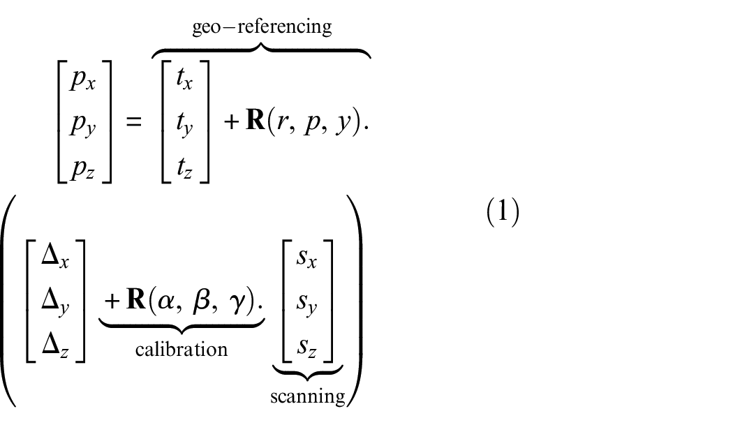
In MLS, however, there are many other sources of systematic deviations. The reason is that point clouds are the result of fusing data from multiple sensors. Each sensor is subject to errors, as is the combination of these. Researchers emphasized that missing functional models and error distributions complicate the uncertainty modeling. 51 Considering the geo-referencing equation (1), we highlight the three main sources of error: geo-referencing, calibration, and scanning itself.
Systematic deviations related to scanning were already part of the discussion in the previous section. Object properties, as well as distance and incidence angle affect MLS point clouds systematically. However, the influence of geo-referencing and calibration is much higher.
Direct geo-referencing means that position and attitude are derived from GNSS (Global Navigation Satellite System), IMU (Inertial Measurement Unit), and odometer data. Theoretically, it is possible to calculate the position with an accuracy at lower centimeter level by incorporating additional GNSS signals from control stations nearby. However, under unfavorable practical conditions in alpine valleys and near tunnels, two geo-referenced MLS point clouds showed deviations of up to 20 cm. 52 The quality of position and attitude depends, among other factors, on location and time, respectively. Geo-referencing thus varies with time, reportedly generating variations of up to 10 cm within 200 m. These discrepancies are the reason why two MLS point clouds of a retaining wall cannot be aligned in terms of rigid-body motion. In other words, neither the ICP method nor the use of ground control points prove suitable to realize a stable reference frame.
System calibration presents another potential error source in MLS. It implies determining the position and orientation of the scanners relative to the IMU coordinate system. The six parameters are three boresight angles
Summary and scope of work
A standard operating procedure for rigorous deformation analysis of laser scanning point clouds does not yet exist. The main reason is that uncertainty information is missing for the scan points, and it is thus impossible to decide whether deviations are significant or explainable by measurement uncertainty. There are numerous research publications on the derivation of covariance matrices of point clouds. Some of them offer complex mathematical approaches that may not be easily applicable in practice.
In the case of MLS, uncertainty modeling is even more complex. Measurement errors are time-dependent, and for some of them the magnitude and distribution is unknown. For example, when calculating the trajectory without costly ground control points, the resulting point clouds may show errors in the decimeter range that vary within a short time. 52 The lack of knowledge about accuracy and precision is why this promising measurement technology has not yet established itself for SHM.
However, in this paper, we propose a working procedure for rigorous deformation analysis of MLS data. We build upon existing work and therefore highlight the overlap of our approach and previous publications.
Under challenging conditions, direct geo-referencing produces trajectory errors that dominate the overall uncertainty budget. Since errors are time-dependent, point cloud registration using ground control points11–14 or point cloud-based methods such as the ICP algorithm 18 will fail in case of MLS. We adopt the idea of Kalenjuk and Lienhart 52 to determine the time-variable deviations between mobile laser scans. We extend the approach by starting a search for the putative deformed objects 38 to be excluded from the point cloud registration.
We co-register point clouds of two scanners of one drive or scans of two drives to remove the major systematic error component in MLS (see equation (1)). The remaining errors are mainly due to the scanning process itself and thus are similar as for TLS. We follow the suggestion by Kuhlmann 51 to quantify uncertainty of MLS empirically. The strategy is to collect a set of point clouds by passing by a scene several times within a short interval and deriving the precision from multiple measurements.
As proposed by Kalenjuk and Lienhart, 52 we use trajectory data to reconstruct the acquisition geometry of MLS point clouds. We exploit this information along with surface parameters such as roughness 38 to build a stochastic model for a commercial MLS system. It enables rigorous deformation analysis of a structure without requiring to collect point clouds multiple times. Such models could therefore bring additional time and cost savings.
Method
Overview
Before going into detail, we first give an overview and clarify notations. Our approach enables rigorous deformation analysis of point clouds captured with a commercial MLS system in a two-stage procedure (see Figure 4). In the quality evaluation and modeling phase, we first determine the quality, i.e. uncertainty of the used MLS system empirically. In the monitoring phase, we incorporate this information to decide whether the computed point cloud deviations represent significant deformations or are due to measurement uncertainty (black, solid rectangle in Figure 4).
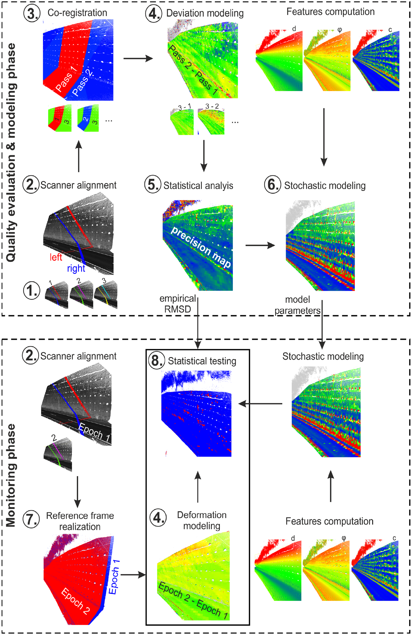
Processing mobile laser scanning data for rigorous deformation analysis requires two phases: the quality evaluation and modeling phase (top), and the monitoring phase (bottom).
In the quality evaluation and modeling phase, the recommended workflow is as follows:
Data collection
When using MLS for capturing structures for the first time, pass by multiple times to collect at least three independent data sets (
Scanner alignment
Before merging point clouds of left and right scanner, check the co-registration quality and correct it if necessary. 52 Otherwise, deformation modeling will be less accurate.
Co-registration
Align the point clouds using the co-registration method that accounts for time-variable geo-referencing errors. 52
Deviation/deformation modeling
Choose a point cloud modeling strategy that works automatically and repeatably. Compute deviations between two point clouds for all
Statistical analysis
The expectation value for the derived parameters is zero. Compute the root-mean-square deviation (RMSD) for each point, region, or segment individually. Since the RMSD values vary in the point cloud, we denote the color-coded point cloud as precision map. The precision map is valid for a given scene, a specific MLS system, and approximately equal conditions (driving lane and velocity).
Stochastic modeling
The last step of this phase is optional, but recommended. Create a stochastic model based on the empirical precision map. Calculate features related to the acquisition geometry and surface roughness. All that is needed is the time-tagged point cloud and the trajectory. Both are typical results of modern MLS systems.
Most processing steps are similar in both phases. Some specialties should be noted in the monitoring phase:
Reference frame realization
The realization of the reference frame requires stable regions for co-registration. Assuming a non-deforming road surface or stable guardrails, we first search for the allegedly deformed structure in a highly automated manner. By doing so, we can exclude it from the co-registration process. However, if nothing can be considered stable, this approach will not work. Then we must rely on the idea that high-frequency trajectory errors occur differently in point clouds of multiple runs and average the results. We have observed both scenarios and report on them in the “Evaluation in practical case studies” section.
Statistical testing
With the empirical precision map available, we can test deformations for significance. If only one point cloud is acquired from a scene, we can leverage the stochastic model learned from another setting to predict precision. The prerequisite is features calculated based on the current point clouds and trajectories.
In the next subsections, we will cover data processing in more detail. We conclude this section with a concise specification list of requirements for data collection and processing.
Scanner alignment
The first thing to check after obtaining geo-referenced point clouds is how well the data of the two scanners match. Remaining calibration errors or uncertainty in the geo-referencing might be reasons for time-variable deviations. If left untreated, the merged point clouds would provide lower accuracy than the scanner data sheets suggest. The solution to align them relies on the same procedure as for two point clouds from different passes. More details on the co-registration method are thus available in the next section.
Reference frame realization
The term reference frame originates from traditional geodetic monitoring. It implies that all measurements have a common coordinate system to which they refer. Although the coordinate system remains the same for multi-temporal mobile laser scans, the point clouds may be shifted due to uncertainties in geo-referencing. Therefore, both the position and the shape are not stable within the coordinate frame. The reason for the latter are the time-dependent measurement errors in MLS.
Realizing a reference frame is thus a matter of obtaining mobile laser scans that overlap in areas where no movements occurred. To accomplish this task, we need to distinguish between two scenarios:
I. Besides the structure to monitor, engineers expect the surrounding environment to be stable. In such a case, we exploit this prior knowledge to co-register the point clouds of two epochs based on these stable areas.
II. Due to mass movements or construction works, there may be no stable region at all. We demonstrate an example of a retaining structure where we faced this challenge. Having this kind of prior knowledge is critical to processing the data correctly. We opted for the workaround of creating a quality-enhanced point cloud by averaging multiple clouds, which proved viable in this case.
Scneario I: We assume two point clouds, a reference cloud
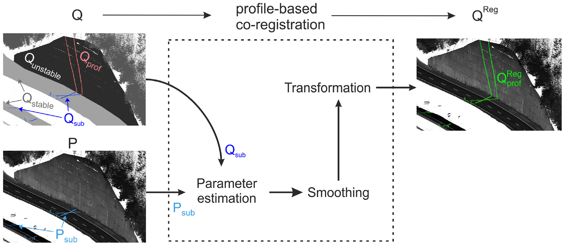
Realization of a reference frame by co-registration of stable regions in two mobile laser scanning point clouds.
The first question is how to decide which regions are stable and which are moving based on point cloud data alone. Unless we receive other information from civil engineers or geotechnical engineers, we assume that the retaining structure could move while, for example, the road and guardrails should be stable. Our strategy is to segment the retaining wall from the query point cloud
Time-variable errors in MLS are why co-registration methods fail to align two point clouds accurately. Despite the time dependency, one may consider the errors constant within sufficiently small time intervals. The strategy is thus to use the nanosecond timing information in mobile laser scans to partition the point cloud.
52
Since most MLS systems use profile scanners, the temporal partitioning will yield subsets
With
Co-registration of
Scenario II: Reference cloud
In such a scenario, possibilities are limited for realizing a reference frame. We opt for the direct geo-referencing solution but enhance the quality by multiple measurement passes. Let us consider a point
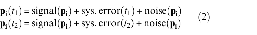
Following the findings of previous work,
52
we must assume systematic deviations due to geo-referencing between two point clouds, no matter whether collected within 5 min or a year. Accordingly, the point clouds recorded in several passes in one epoch will be influenced by systematic errors differently. Although the distributions of the errors are unknown,
51
we expect
It is worth mentioning that this strategy neglects the atmosphere as a traditional influence factor. In contrast to tachymetric observations, the mapping geometry remains the same along the entire wall. Even for tall structures, the distances are no greater than 35 m (c.f. Figure 9). Range distortions are thus negligible. Moreover, one can reduce refraction-related angle distortions by scheduling the mapping campaign on cloudy days.
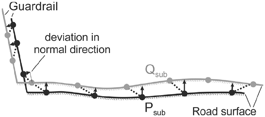
Our strategy is to reduce the geo-referencing-related systematic component by scanning the scene multiple times and averaging the point clouds. However, we do not average the coordinates of corresponding points individually, but use a modified version of the profile-based co-registration method (see Figure 5). The motivation for this procedure is robustness and precision in the presence of noise. In general, the workflow is similar to the one presented in “Scenerio I” (see also Figure 5). In a nutshell, it adopts the following procedure:
Establish direct point correspondences by searching for the nearest neighbors in both MLS point clouds,
Perform temporal partitioning,
Estimate transformation parameters by minimizing point cloud deviations in normal direction,
Smooth the transformation parameters and
Apply the transformation to both point clouds. More precisely, rotate both clouds by half the angle, but in opposite directions, and shift them by half the translation vector, each with a different sign.
The proposed procedure reduces systematic deviations between two point clouds. Since we captured at least three laser scans of each structure in each epoch, we can apply the method to all
Deformation modeling
Through the previous processing steps, the point clouds
Our strategy is to model the deformation pattern of the entire structure as a composite of many rigid-body motions. The procedure consists of two steps (Figure 7). We first subdivide the mobile laser scans into point groups that adhere to object boundaries. Then, we estimate the translation and rotation parameters that best align the surface patches of cloud
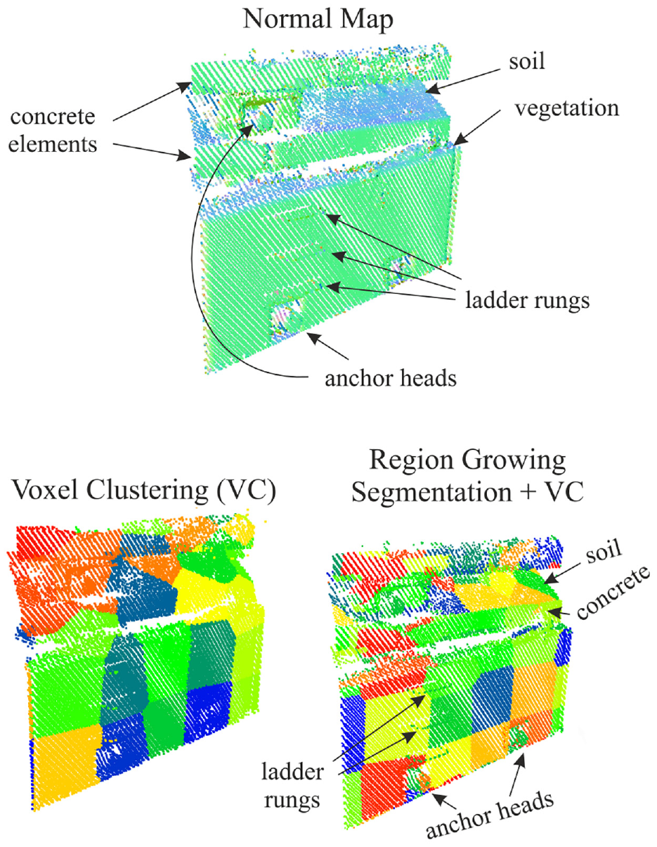
Visualization of normals of a cloud of a crib wall in the HSV color space, labeled as normal map (top); voxel clustering of the cloud with a voxel size of 1 m (bottom left); and cascading region growing-based segmentation and voxel clustering (bottom right) to obtain small point sets that adhere to object boundaries (c.f. object details in normal map). HSV = hue, saturation, value.
Step 1: Point cloud partitioning
A prerequisite for the partitioning algorithm is surface normals. We compute them at each point using the surrounding neighbors within a specified radius. The radius choice depends on the structure’s surface and the minimum feature size to resolve (see normal map in Figure 7). By decreasing the search radius, the object description becomes more detailed, but the variance also increases. Considering retaining wall C with 30 cm wide reinforced concrete elements or retaining wall B with 30 cm wide block joints, we propose a radius of 15 cm for normals computation. We leverage the descriptiveness of normals for point cloud segmentation. Compared to prior work,
38
we do not aim to precisely cluster groups into perceptually meaningful regions. The reason is that the strategy would fail in practice for structures like retaining wall C (Figures 2 and 7). The elements are thin, there is heavy vegetation, and with a wall height of 16 m, there are also differences in the point density between the top and bottom of the structure. Therefore, we instead apply a generous angle threshold of 5°–10° to obtain over-segmented point sets
Next, we spatially cluster the segmented point cloud
Step 2: Estimating transformation parameters
Given a clustered reference point cloud
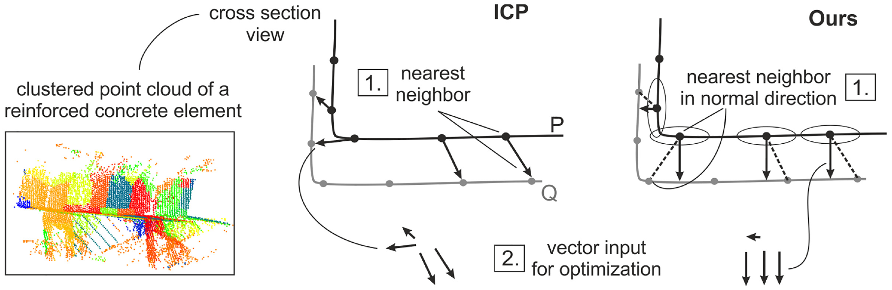
Deformation modeling of a concrete element of retaining wall C: clustered point cloud (left) and visualization of the working principle using Iterative-Closest-Point (ICP) (middle) and our algorithm (right).
Our method for estimating transformation parameters works differently. Like the M3C2 algorithm, we search for the corresponding points within a cylinder whose axis is aligned with the surface normal at this point (dashed line in Figure 8, right). Note that surface normals
The point sampling has less influence on the orthogonal distances than on the 3D displacements.
Much of the transport infrastructure consists of flat surfaces. Typical deformation patterns occur in the lateral direction or cause structural tilting that is measurable perpendicular to these surfaces.
For each point
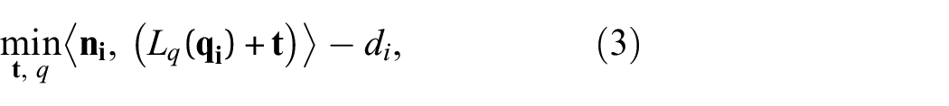
we realize a minimization of orthogonal distances between
In summary, our method for deformation modeling incorporates concepts from M3C2 and the ICP algorithm. The basic idea is to compute transformation parameters between two point subsets, just as the ICP algorithm does. However, our algorithm differs in two aspects. First, we identify corresponding points as the closest only if they lie within a cylinder whose axis coincides with the surface normals. This idea originates from the M3C2 algorithm, which searches for corresponding points orthogonal to the scanned surface. The second difference is that we minimize these orthogonal distances instead of the Euclidean distance. The benefit of doing so is less sensitivity to varying point sampling and in-plane movements. As a result, we obtain translation and rotation parameters in 3D space.
Stochastic modeling
So far, we have described the first three steps of both phases, the quality evaluation, and monitoring phase (see Figure 4). We successfully aligned point clouds of the left and the right scanner and co-registered the mobile laser scans of two passages. Moreover, an automatic procedure for modeling 3D deformations is at our fingertips. Now all is prepared for the derivation of uncertainty in MLS. Of the three systematic sources of error in MLS (see “State-of-the art in laser scanning and deformation monitoring” section), the proposed preprocessing steps eliminate the geo-referencing and calibration component. These two are specific to MLS and dominate the overall error budget of point clouds.
After their elimination, we can focus on the remaining source of error, namely the scanning process itself. The strategy is as follows. In the course of data collection, scan a retaining structure three times minimum. Compute the lateral displacements
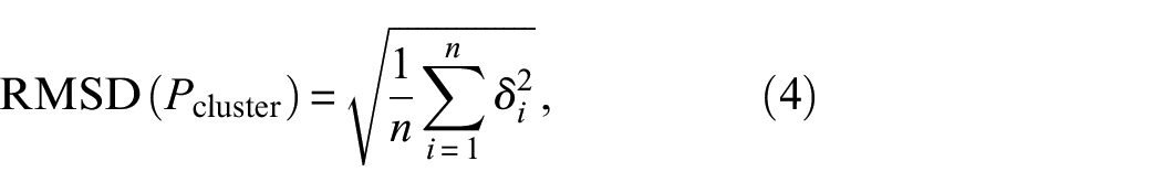
with
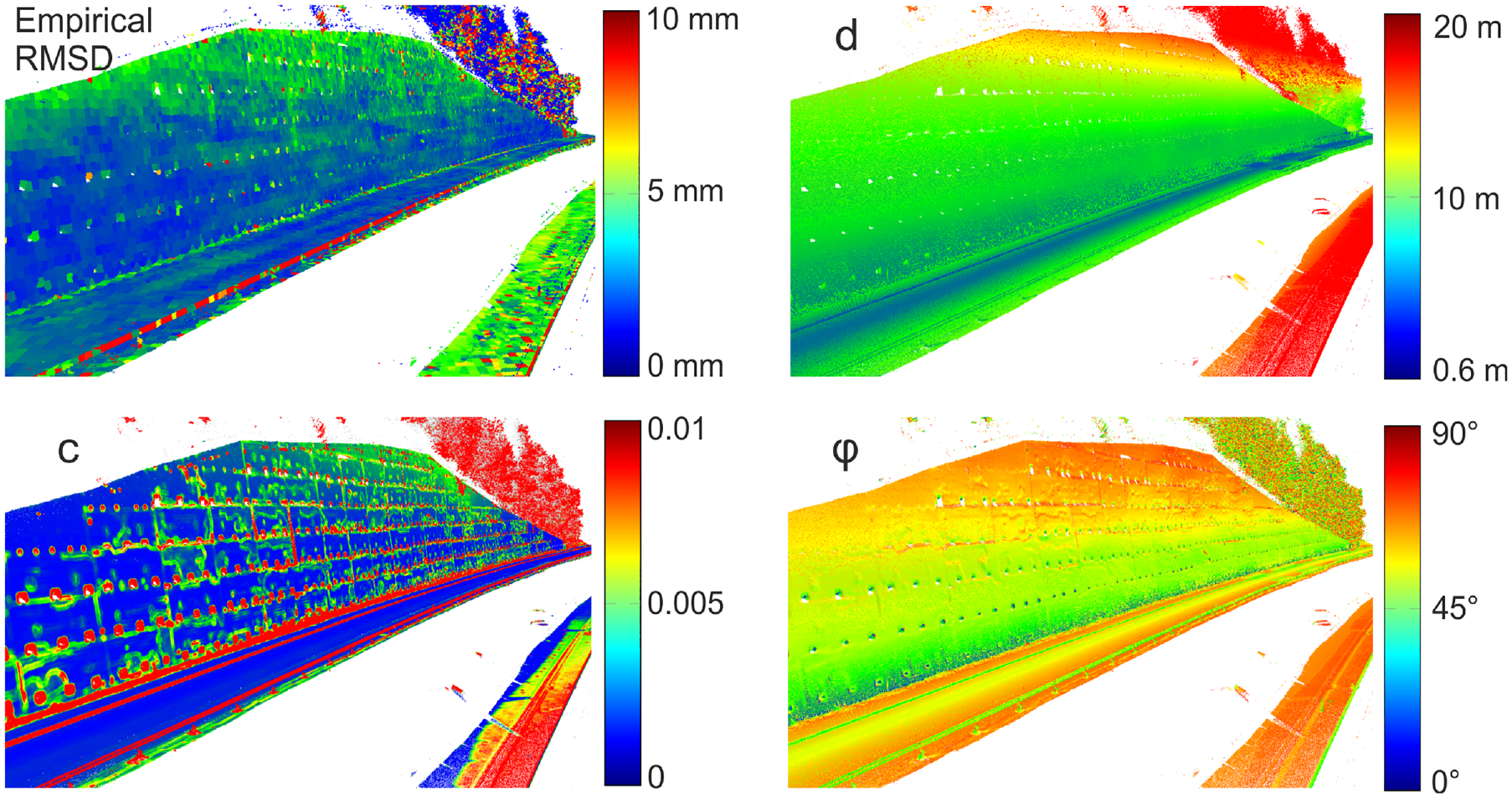
The precision map correlates with surface properties and the acquisition geometry. Visualization of the key parameters for retaining wall A: empirical root-mean-square deviation (top left), surface curvature
So far, researchers have investigated the factors influencing laser scanning in elaborate experiments under controlled conditions. Here, we show how the influencing factors (see Figure 1) can be also derived directly from MLS data. The requirement is the trajectory, that is, position (
We adopt the shorthand notation of the geo-referencing equation (1)

and rearrange it to


and the incidence angle
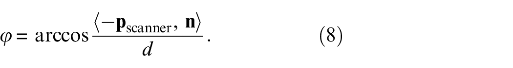
Principal component analysis is the mathematical basis for calculating surface normals, which provide valuable byproducts for another crucial point cloud feature. The ratio between the smallest eigenvalue and the sum of eigenvalues describes the variation of the surface. This measure is also commonly referred to as surface curvature
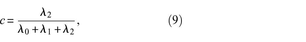
whereas
Equations (7) to (9) provide the formulae to compute three features for each individual point. Similar to the idea of Extended Gaussian Images for visualizing surface normals,
54
we interpret the three features as point coordinates in
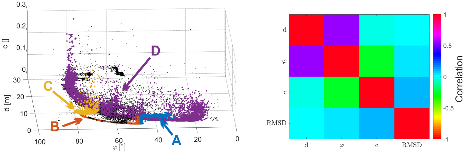
Correlation of point features and the root-mean-square deviation (RMSD) for retaining wall A: 3D visualization of the features as point cloud with specific areas highlighted with A-D (left) and the correlation heat map of features and RMSD (right).
The correlation between point features and RMSD is much lower. So the question is whether we can use these features to build a model that estimates RMSD for scenes that have only been scanned once. As the three features and the target variable appear to have a non-linear relationship, we aim for a non-parametric model. Among the supervised machine learning algorithms, the random forest (RF) regression algorithm promises good predictive performance with little hyperparameter tuning.
55
Nevertheless, before feeding the RF with data, we first preprocess the feature cloud. Let us consider a cluster
Intuitively, the trained RF model provides rules on partitioning the feature space
Summary—requirements for data collection and processing
We propose a method for rigorous deformation analysis of MLS data. It is not state-of-the-art and requires multiple processing steps that can be automated. To sum up, following requirements apply for the data collection or delivery, respectively:
Point coordinates with time stamp:
Point clouds separated by left and right scanner
Information from geotechnical or civil engineers on stable areas
Three collected data sets if nothing is expected to be stable near the structure
Uncertainty information as
○ a valid stochastic model for the MLS system and the scene or
○ three point clouds of one epoch to determine the precision map empirically for the MLS system and the scene
Trajectory data exported with the highest possible frequency and including timing information:
The lever arm
The method requires following considerations regarding data processing:
Merging data without checking the co-registration of left and right scanner will introduce additional uncertainty
MLS point clouds suffer from time-variable errors
The proposed method performs a profile-based co-registration that accounts for these time-dependent errors
A prerequisite is that road surface and inventory are stable near the structure in-between the data collections
If nothing is expected to be stable due to, for example, construction works, one can obtain a stable reference frame by averaging multiple data collections of one epoch, albeit with lower accuracy
The computationally most intense processing step is calculation of surface normals
A complex structural deformation pattern is approximable by a composite of rigid-body motions of many small surface patches
Focusing on the deformations perpendicular to the structure’s surface
Multiple data collections of one epoch allow deriving the empirical RMSD
If a stochastic model is available from previous campaigns, one can predict the precision map, a color-coded point cloud with RMSDs using point cloud features
The time-tagged trajectory and point cloud, enables us to compute two relevant point cloud features for each point: distance and angle of incidence
The third feature is surface curvature (or roughness), described by the ratio of eigenvalues.
Finally, we can formulate the null hypothesis
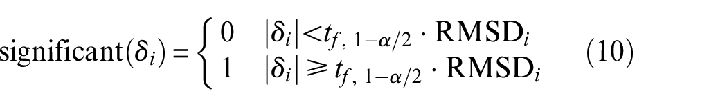
The choice of
Evaluation in practical case studies
We present the application of our method to three practical use cases. Retaining structures A, B, and C provide examples of the feasibility of rigorous deformation analysis of MLS data and the associated challenges. The selected three differ in surface properties, structural type, and, thus, the deformation behavior. In this section, we, therefore, focus on three key aspects of the method:
The complete workflow: We show the results from intermediate steps and evaluate the accuracy using geodetic surveys for retaining structure A.
The efficiency: Building upon the results from the previous example, we highlight how to increase efficiency further for structure B by using a stochastic model.
The large-scale deformation case: While most structures show little to no deformations, retaining structure C did experience extensive deformations, including its surrounding. Such a case is rare and poses challenges to processing MLS data.
Retaining structure A—evaluating the complete workflow
Retaining structure A is an ideal testbed. With its 18 m height, it stabilizes a slope next to a state road that is less heavily trafficked than the highway next to it. However, failure would affect both traffic routes, making the maintenance of the structure of great importance. Although such failures are seldom, an incident on an Austrian Highway in 2012 57 raised the operator’s awareness. The last inspection attested retaining wall A to be in a poor structural condition. The main reason was the concrete surface, which spalls and poses a danger to pedestrians using the nearby sidewalk. Another problem was the old anchors, originally not designed for detailed inspections. Their exact condition and, thus, the expected total service life of the structure were unknown. Parallel to ongoing geodetic monitoring, we conducted total station surveys from 3 setup stations to 19 prisms (see Figure 3) on our own. Hence, the classical rigorous deformation analysis served as a benchmark for our proposed, novel approach. The MLS campaigns took place on November 27, 2019 and November 10, 2020. During road closures, we drove by the structure four times, twice in each direction at about 40 km/h.
Precision map
Using the four MLS point clouds, we computed the RMSDs for each cluster (see equation (4)). Figure 11 top depicts the distribution of the RMSDs in the empirical precision map. The bottom visualization of Figure 11 shows the modeled precision map. It represents the prediction of the RF regressor trained on the three features,
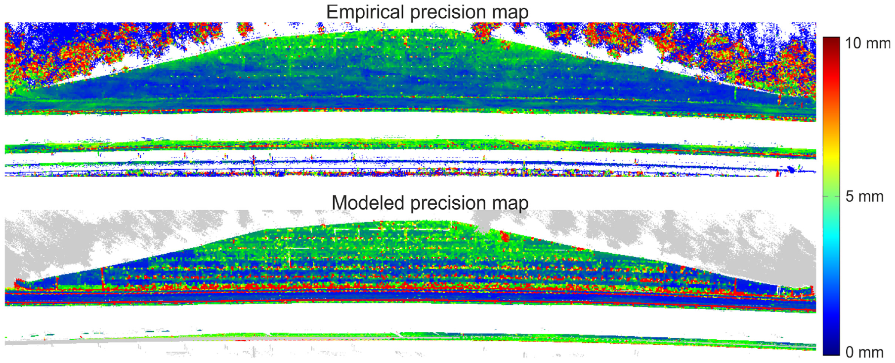
Precision of MLS monitoring retaining structure A: empirical (top) and modeled (bottom) precision map.
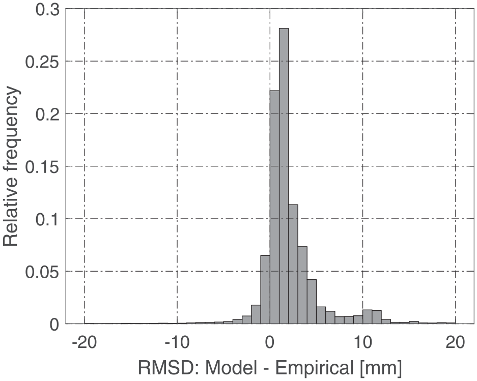
Histogram of differences of modeled and observed root-mean-square deviations for retaining wall A.
Deformation and significance map
Following the assessment of geotechnical engineers, we considered road surface and infrastructure inventory stable for co-registering MLS cloud from 2019 and 2020. The deformation map obtained from the two MLS surveys is visible in Figure 13, left.
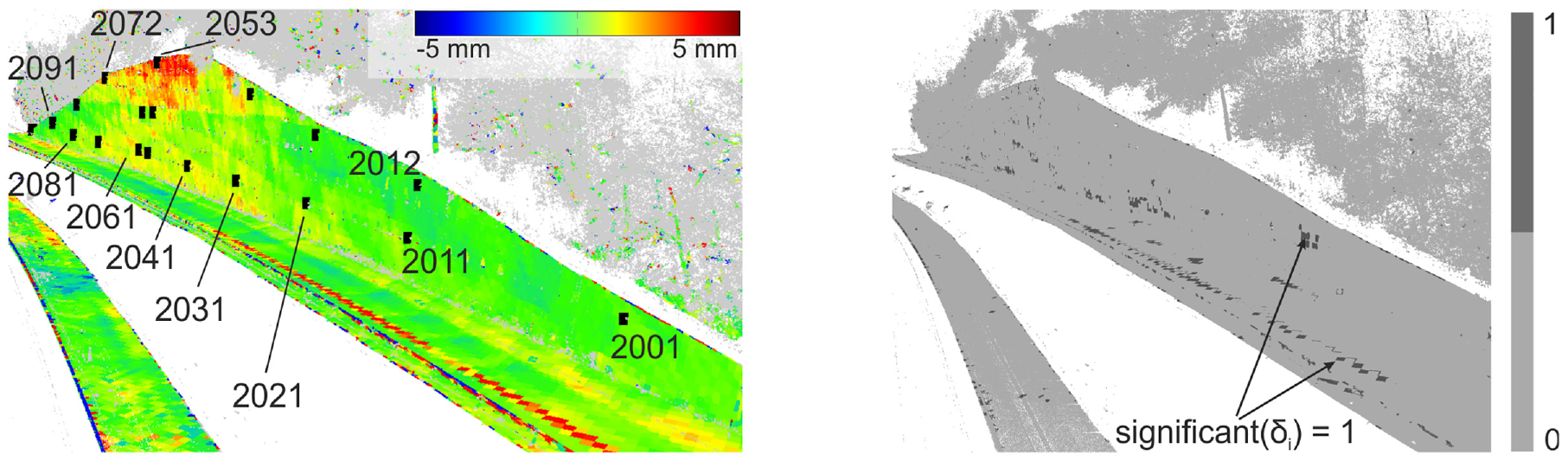
MLS-based rigorous deformation analysis of retaining wall A for the period between November 2019 and November 2020: lateral displacements with locations of geodetic reference targets (left) and binary plot indicating significant displacements (dark gray, right).
The color bar is limited to ±5 mm, and yet most parts of the plot are green. However, the red pattern at the top of the wall indicates positive lateral displacements of approximately +5 mm. The direction of displacements follows the convention defined by the reference frame for geodetic monitoring. In this case, positive deformations mean displacements toward the slope, that is, away from the road and highway. We have observed seasonal variations of this magnitude with total stations, but the variations shown are due to uncertainties in laser scanning. We can draw this conclusion with the precision map at our fingertips (Figure 11). Using either the empirical or modeled map, we can interpret the point cloud discrepancies and classify them as significant or insignificant. The binary significance map (as visualization of equation (10)) in Figure 13 (right) identifies most of the structure as not displaced between 2019 and 2020. Individual clusters flagged significant may be considered outliers.
Benchmarking MLS using geodetic surveys
The black dots and numbers in Figure 13 (left) visualize the location of the 19 prisms. For each of them, we plot the lateral displacements obtained from conventional and MLS monitoring in Figure 14. The graph additionally shows the confidence intervals for both methods. Since we conducted geodetic surveys from three setup stations (see Figure 3), we derived the 95% confidence of the lateral displacements. Thanks to our precision map, we can plot the 95% confidence region for MLS by scaling the precision map by
Rigorous deformation analysis of structure A at the location of the 19 prisms obtained by static, geodetic moni-toring (top) and MLS monitoring (bottom); deformations are significant for points whose 95% confidence bands do not overlap with the zero displacement line.
To sum up, the MLS approach enables monitoring the spalling, rough concrete surface of structure A with a precision of better than 5.4 mm. The established stochastic model predicts RMSDs at the structure that conform in the millimeter range to empirical values. The absolute displacement values of the 19 points agree with geodetic surveys within 5 mm.
Retaining structure B—increasing efficiency
Retaining structure B is representative of the many anchored structures of medium height in the Austrian highway network. 38 It consists of several anchored concrete elements of 5.4 m × 5.4 m size with a relatively smooth surface. A local surveyor performs geodetic monitoring of 19 retro-reflective points twice a year. During these measurements, the road administration closes one lane of the busy highway. For safety and efficiency reasons, we thus consider the deliverables from the external surveyor as our benchmark. The dates of the geodetic and MLS surveys (November 27, 2019 and November 10, 2020) roughly coincide at both epochs.
Time savings by reducing amount of data
To prevent any significant impediment to the traffic flow, we drove past the structures at the minimum permissible speed of 80 km/h. So we moved twice as fast as when scanning structure A, completing the point cloud acquisition after 7 s. A single pass with such a short data collection is sufficient to apply our workflow for deformation monitoring. The underlying idea is to predict the precision map of structure B based on the learned stochastic model from structure A. The transfer of the learned relations between the features and the RMSDs from A to B (and C), works well, as we have shown in the Section “Evaluation of the stochastic model” in the Appendix. By reducing the number of scans needed, we can spare time in collecting data and processing the precision maps.
Maintaining the workflow
The rest of the workflow is the same as for structure A. We first derive the deformation map (Figure 15, top left). Again, we received the information that, except for the structure, everything else should not have moved between the two epochs. Accordingly, we established the reference frame for comparison by co-registering the point clouds over stable regions. Then, we incorporated the modeled precision map (Figure 15, bottom left) to statistically test the deformations (lateral displacements) for significance (Figure 15, right).
The three key components of rigorous deformation analysis of structure B using mobile laser scanning (MLS) data: deformation map (top left), the modeled precision map (bottom left), and the binary significance map (right).
Compared to structure A, the acquisition geometry is more favorable for structure B. Note the larger scanner-to-object distance at a highway and the lower height (Figure 2). The wall points thus result from scanning at roughly equal distances and angles of incidence. As a result, the RMSDs do not differ considerably between the toe and top of structure B (see precision map in Figure 15). Regions of high surface curvature, including joints and vegetation, are clearly evident in the modeled precision map.
The deformation map (Figure 15, top left) shows a specific pattern for the highway and the structure (same colorbar limits as for structure A). One could spot local settlements at the pavement or displacements at the top of the wall, but we can classify them as insignificant after statistical testing.
Maintaining accuracy and completeness
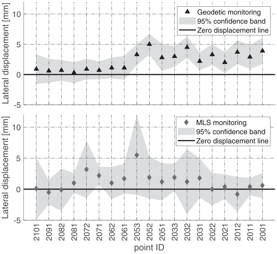
We evaluated the MLS approach based on the external geodetic surveys of the 19 prisms visualized as block dots in Figure 15 (top left). Since there were no uncertainty values stated in the monitoring report, we assumed a constant precision of ±1.5 mm for all points. According to the statistical test, the geodetic surveys revealed significant displacements for point 9.0 only (Figure 16, top), whereas MLS flagged all points as unmoved (see also significance map in Figure 15). Except for the mentioned point 9.0, MLS and geodetic surveys provide lateral displacements that deviate less than ±5 mm.
Rigorous deformation analysis of structure B at the location of the 19 prisms obtained by static, geodetic monitoring (top) and mobile laser scanning (MLS) monitoring (bottom); deformations are significant for points whose 95% confidence bands do not overlap with the zero displacement line.
One interesting observation is that data points are missing for both methods. According to the monitoring report, the bi-reflective targets of points 7.0, 8.0, and 8.1 were not available at epoch 2. They must have broken down sometime in the summer or fall of 2020, so the trace of their displacements was lost. MLS provides complete field information and does not rely on targets and sensors installed on the surface. However, a weakness of laser scanning becomes evident at points 7.2 and 8.2. These two points are located above the wall where shrubs obstruct the line-of-sight to them (Figure 15, top left). With dense vegetation in front of the wall (as is often the case for crib walls), quality decreases drastically, and may result in no displacement values being determined at all.
Although structure B defines a typical example among thousands of objects in the Austrian highway network, the use case provided additional insights:
The proposed procedure does work with one point cloud per epoch only. It is not necessary to pass by multiple times and derive precision maps empirically. We can model it based on point cloud features.
The driving speed has little to no effect on the accuracy of the lateral displacements.
The precision of MLS-based monitoring depends on surface smoothness and acquisition geometry.
Geodetic monitoring can lose track of displacements when optical targets break and are no longer recoverable. MLS provides deformations independent of any installations, but it may require time-consuming pruning operations if there is heavy vegetation (especially for crib walls as structure C).
Retaining structure C—the large-scale deformation case
Retaining wall C is located along an Austrian highway. It is an anchored crib wall of 330 m in length and 14 m in height. The structure consists of many precast reinforced concrete elements, each 3.4 m long and 0.3 m high. The composite of soil and anchored parts provides the supporting effect. Hence, trees and shrubs grow between the artificial elements and cover the front of the wall. Crib walls thus proved to be more challenging than anchored structures with concrete surfaces, for exmaples, structures A or B. The potential deformation behavior is also more complex, as movements can occur very locally. Some elements may rigidly shift if an anchor fails, or individual components may break due to their slender design if additional loads arise.
Background information
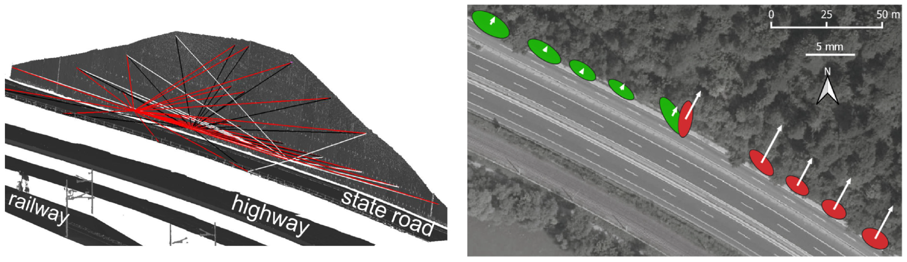
In our analyses, we divide structure C into two parts: C1 and C2 (Figure 2). The reason is that C1, with its 150 m, and C2, with its 180 m length, behave differently. Currently, a new tunnel with two tubes is being built, crossing under the highway and the retaining structure at a depth of 100 m (see white lines in Figure 17). As a result of the tunnel construction, terrain settlement has been observed in the surrounding area. To better assess the structural response, engineers installed total stations to permanently monitor the deformations at 94 prisms at hourly intervals during construction for a period of more than 1.5 years. We received the measurement data for evaluation at the exact time of our MLS surveys on November 27, 2019 and April 12, 2022. The observed lateral displacements (white arrows in Figure 17) show increased deformations for C2, while C1 remains stable. The west tube defines the transition zone between the two structures, C1 and C2, and the moving and stable zones.
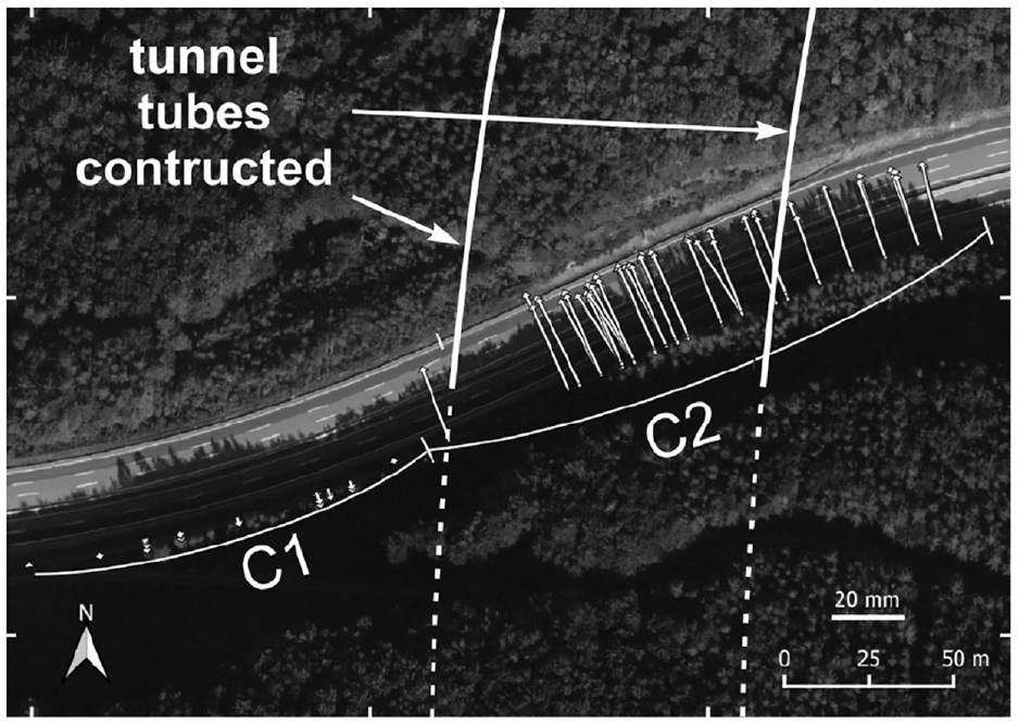
Orthophoto of the scene around retaining wall C: the arrows indicate the displacement vectors obtained from geodetic monitoring between the epochs December 2019 and April 2022; the white solid lines represent the current state of construction of the tunnel tubes as of April 2022.
Workflow adaptation
With the prior knowledge about the structure’s behavior, we could not proceed as with retaining wall A and B. The problem is that the profile-based co-registration method would compensate for the local settlements, when presuming stable surfaces in the point clouds. This approach would thus incorrectly suggest no settlements in the area of C2.
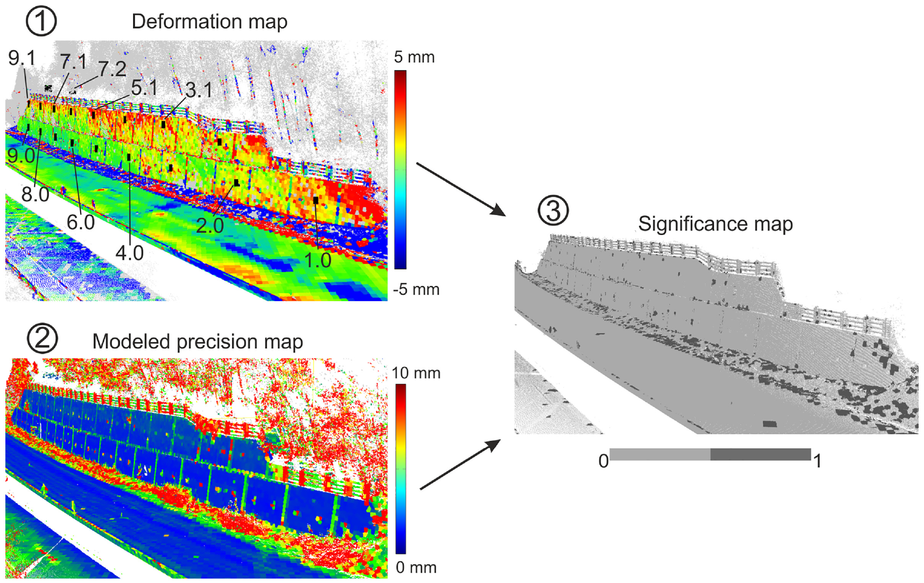
In such a case (see Scenario II in Section “Reference frame realization”), we acquire multiple datasets and compute a quality-enhanced point cloud per epoch. The proposed method averages the collected point clouds and thus minimizes low and high-frequent systematic trajectory errors. This strategy proves to be particularly feasible when the expected deformations are in the centimeter range. The remainder of the workflow is the same as for retaining wall A or B, as Figure 18 shows. We predict the precision map (2) based the stochastic model from structure A to test the deformation map (1) for significance (3).
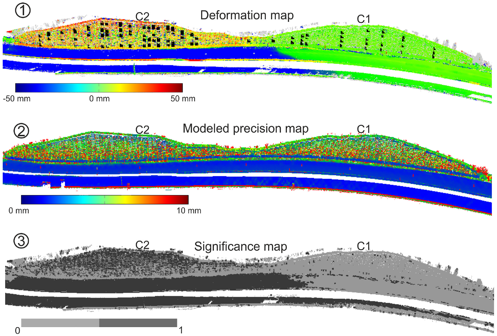
The three key components of rigorous deformation analysis of structure C using mobile laser scanning (MLS) data of November 2019 and April 2022: deformation map (top), the modeled precision map (middle), and the binary significance map (bottom).
Benchmarking MLS using total station data
At first glance, the deformation map resembles the behavior observed by the total station measurements (c.f. Figures 17 and 18). C1 shows almost no movements, while the comparison of the point clouds indicates extensive deformations for structure C2 and the road next to it. At the pavement, the two epochs differ by a maximum of −90 mm, roughly corresponding to the −80 mm settlements reported by geodetic monitoring. The compliance is remarkable, considering that the two quality-enhanced point clouds were not registered to each other. According to the statistical tests, C2 deformed, and the nearby road settled significantly (see significance map in Figure 18, bottom).
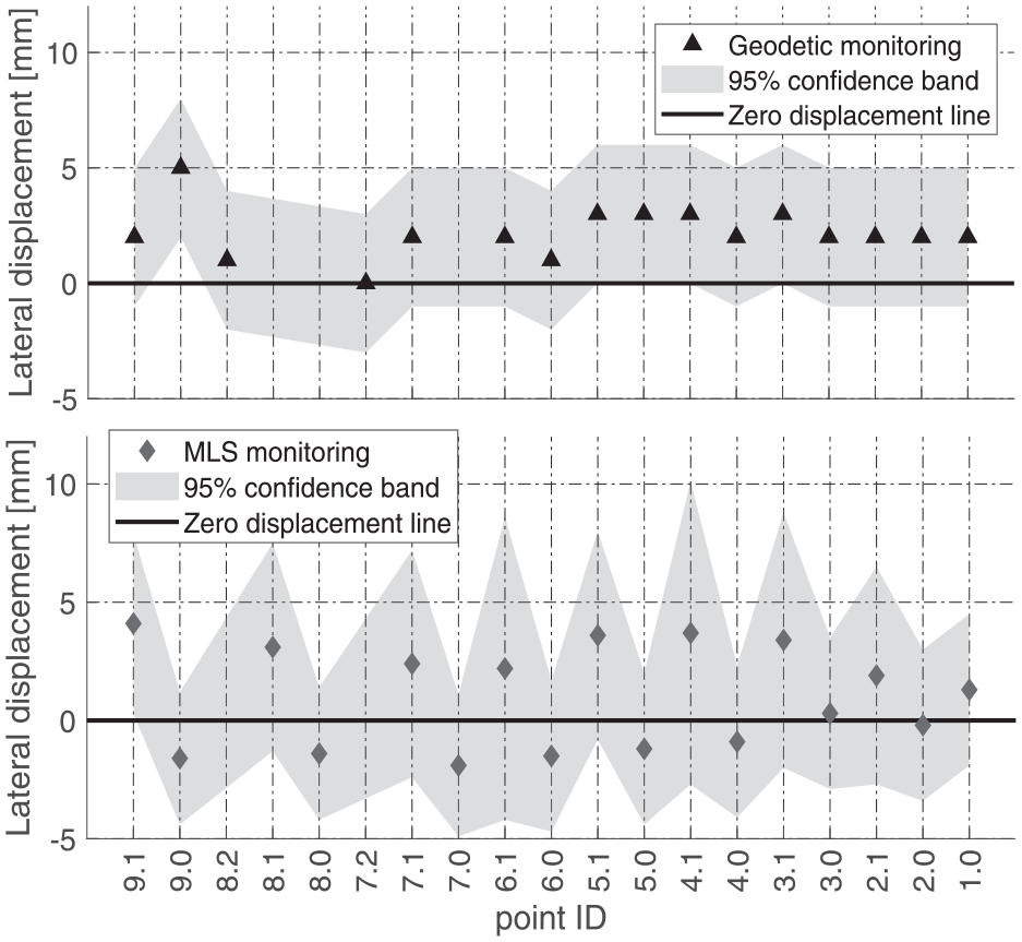
Figure 19 depicts the lateral displacements of the 94 prisms observed with geodetic measurements and MLS between the epochs November 2019 and April 2022. The prisms are numbered in direction from C1 to C2. For structure C1 (right of dashed line), lateral displacements are below 5 mm and thus at the limit of being flagged significant. At the transition zone between C1 and C2 (dashed line), where the west tube crosses the structure, the point movements increase up to 30 mm. The rest of the points at structure C2 indicates significant displacements of +20–+30 mm toward the highway. Note that we again assumed a precision of 1.5 mm for the statistic testing of geodetic measurements.
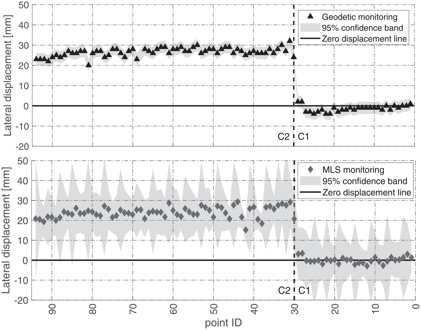
Comparison of mobile laser scanning (MLS)-based (gray) and static, geodetic monitoring (black) at the locations of the target prisms at structure B; the bars indicate the 95% confidence levels.
The results of the MLS approach reflect the deformation pattern described (Figure 19, bottom). The confidence intervals of the C1 points overlap the zero displacement line, meaning that they have not moved statistically. By contrast, the rigorous deformation analysis of the MLS data attests 60 out of 63 points (corresponding to 95%) at C2 having displaced significantly. The magnitude of displacements ranges from +20 to +30 mm. Accordingly, the two methods agree better than ±10 mm for most points and as the confidence bands intersect (if overlayed), the differences between the MLS and geodetic monitoring are insignificant. It is worth mentioning that the precision of the MLS approach is worse for the thin concrete elements partly covered by vegetation (compared to structures A or B), so the confidence intervals are larger (e.g., ±15 mm).
Retaining structure C proved to be a valuable case study. Most of the infrastructure objects investigated showed little to no movements. Based on structure C, we could show the capability of MLS for detecting large-scale deformations. The obtained results are remarkable, since 95% of the displaced points could be identified as such. Albeit a challenging object surface with vegetation, the achieved accuracy is better than 10 mm. Note that for the evaluation at the position of the 94 prisms, we averaged values from adjacent voxels to obtain the lateral displacements at this point. Due to the wider confidence bands (compare Figure 19, top and bottom), MLS will not replace the more precise geodetic monitoring in all situations. The latter will remain the monitoring technique of choice in safety-critical situations. However, MLS has proven to provide accurate and unbiased results. It offers great potential for large-scale application in efficiently assessing the condition of many objects in transport infrastructure.
Conclusion
In this article, we have proposed a method for monitoring the structural deformations of retaining structures in a transport network using MLS. The idea is to leverage the fast data collection capability, apply efficient, automated point cloud processing, and thus establish a working procedure that scales to many objects. Remarkably, it is not limited to specific hardware but is compatible with commercially available MLS systems from four major manufacturers. We defined the requirements regarding data collection, delivery, and processing. Accordingly, following the provided guidelines, one can contract external service providers for data collection and will still obtain comparable datasets.
The proposed processing pipeline follows two basic concepts. First, remove systematic deviations, including geo-referencing and calibration errors. Second, determine the remaining discrepancies through multiple passes empirically. By incorporating the uncertainty into the deformation monitoring, we can test the modeled deformations for significance, conforming to the principle of rigorous deformation analysis. We also showed a way to circumvent the need for repeatedly scanning an object at each epoch. It is possible to predict the uncertainty of a point cloud by a supervised stochastic model based on the three main features: scanner-to-object distance, angle of incidence, and surface roughness.
We presented three case studies in which geodetic surveys served as benchmark. In the case of a more or less smooth object surface, the precision and accuracy proved better than 5 mm. An anchored crib wall that experienced large deformations of almost 100 mm turned out challenging for modeling deformation from the MLS point clouds. While the accuracy achieved is lower compared to the other two objects, our method successfully identified the same regions as moved as the geodetic monitoring measurements. This result is remarkable and highlights the potential of MLS for infrastructure maintenance.
In safety-critical cases, MLS will not replace other, high-accurate measurement techniques in SHM. However, we presented a time-efficient working procedure to inspect many structures and identify potentially defective ones in road and railway networks. We intend to give the inspecting engineer information at hand to assess the structure’s health condition more objectively.
Footnotes
Appendix
Acknowledgements
We thank the industry partners for conducting the MLS surveys and the road administrations for the escort service.
Declaration of conflicting interests
The author(s) declared no potential conflicts of interest with respect to the research, authorship, and/or publication of this article.
Funding
The author(s) disclosed receipt of the following financial support for the research, authorship, and/or publication of this article: The Austrian Federal Railways (ÖBB), Austrian Highway Agency (ASFiNAG), the Austrian State Departments, and the Austrian Research Promotion Agency (FFG) supported the research project (FFG project SaRAS, no. 888905).