Point cloud clustering and outlier detection based on spatial neighbor connected region labeling

Abstract

Clustering analysis is one of the most important techniques in point cloud processing, such as registration, segmentation, and outlier detection. However, most of the existing clustering algorithms exhibit a low computational efficiency with the high demand for computational resources, especially for large data processing. Sometimes, clusters and outliers are inseparable, especially for those point clouds with outliers. Most of the cluster-based algorithms can well identify cluster outliers but sparse outliers. We develop a novel clustering method, called spatial neighborhood connected region labeling. The method defines spatial connectivity criterion, finds points connections based on the connectivity criterion among the k-nearest neighborhood region and classifies connected points to the same cluster. Our method can accurately and quickly classify datasets using only one parameter k. Comparing with K-means, hierarchical clustering and density-based spatial clustering of applications with noise methods, our method provides better accuracy using less computational time for data clustering. For applications in the outlier detection of the point cloud, our method can identify not only cluster outliers, but also sparse outliers. More accurate detection results are achieved compared to the state-of-art outlier detection methods, such as local outlier factor and density-based spatial clustering of applications with noise.

Introduction

Clustering is one of the major data mining methods for knowledge discovery, which plays an important role in analyzing these data. Clustering typically divides a dataset into groups of similar objects by minimizing the similarity between objects in different clusters and maximizing the similarity between objects within the same cluster. It is often helpful for identifying the underlying structure of datasets and informative patterns in subgroups of the data. Clustering is a versatile unsupervised learning method that can be used in several ways including pattern recognition, marketing, document analysis and point cloud processing.^1,2 Cluster analysis is applied to identify homogeneous and well-separated groups of objects in datasets. Therefore, it plays an important role in many fields of business and science.

Usually, most of the collected real-world datasets include noise. Sometimes, clusters and outliers are inseparable for those datasets with cluster outliers. Point cloud outlier is a dataset that deviates from measured objects. The existence of outliers directly influences point cloud processing results such as curvature calculation, normal estimation, registration, feature extraction and surface reconstruction. Therefore, the detection and removal of outliers have a great impact on the point cloud processing. Outlier detection is also important in data mining with numerous applications in business and science. Therefore, it is necessary to treat clusters and outliers the equal importance in the data analysis.

In recent years, many clustering algorithms have been proposed, such as hierarchical, K-means, density-based spatial clustering of applications with noise (DBSCAN),^3–10 but we observed that most of the clustering algorithms are computational complexities and cannot be used to detect sparse outliers. Therefore, they are very time-consuming in analyzing large data. Thus, we propose a novel data clustering algorithm called spatial neighborhood connected region labeling (SNCRL) which is inspired by the connected region labeling algorithm used in two-dimensional (2D) image processing. A k-nearest neighborhood is first constructed based on the KD tree. The criterion of spatial connectivity is then defined with difference from the pixel connectivity. After that, SNCRL categorizes points to the same cluster based on the connectivity criterion. The proposed method is applied for data clustering and outlier detection of the point cloud with the following advantages:

1. Only one parameter k (k-connectivity) is needed, which is easy to select an appropriate value.

2. The algorithm is simple in calculation that is different from most of the existing cluster algorithms. It can be used for large data clustering and outlier detection.

3. The algorithm can be well used for not only cluster outlier detection, but also sparse outlier.

The remainder of this paper is organized as follows. Section “Related work” introduces the related work of clustering and outlier detection. In section “Proposed method,” the image processing of the region labeling algorithm and our method for data clustering is presented. The method performance is evaluated and analyzed in section “Experimental results and analysis.” Section “Conclusion” concludes this research.

Related work

Many clustering algorithms have been proposed, and these algorithms can be broadly classified into three types: partitioning, ³ hierarchical ⁴ and density-based ⁵ algorithms. Partitioning algorithms classify a database containing n objects into K clusters. In general, partitioning algorithms start with an initial point and then optimize the clustering result using some control strategies. ¹ The most widely used partitioning algorithm is the K-means clustering proposed by Lloyd ⁶ that minimizes the intra-cluster distance. Its computational complexity is K × M × N × i, where K is the number of clusters, M is the number of points, i is the number of iterations and N is dimensions of the vector. ¹ The hierarchical clustering has two basic types: agglomerative and divisive. Generally, the complexity of hierarchical clustering is O(n)³ at least, ¹ where n is the number of points, which is time-consuming for large dataset clustering. DBSCAN^5,7 is a classic density-based clustering algorithm to discover clusters of arbitrary shapes, and its computation complexity is O(n log(n)) based on KD tree searching. ¹ These clustering algorithms are very complex and time-consuming in applications. In recent years, some new clustering algorithms were proposed, such as optimizing K-means clustering, ⁸ dynamic immune clustering, ⁹ dynamic clustering based on the particle swarm optimization, ¹⁰ automatic clustering with differential evolution ¹¹ and mean shift clustering. ¹² However, their computational complexities are still very high. Thus, these methods are very time-consuming in analyzing large data.

Domingues et al. ¹³ made a full overview of the outlier detection. Outliers can be classified into two types: sparse and cluster outliers; they are randomly distributed around the object without any topological structure. The sparse outliers are single points deviated from the measured object. Cluster outlier is a cluster dataset that consists of more than two points. The outlier detection methods are mainly divided into four categories based on distribution, distance, density and clustering. In distribution-based methods, the distribution of points that deviate from a standard distribution is regarded as outliers. ¹⁴ Therefore, if we know distribution of the point cloud, outliers can be detected effectively. However, distribution-based methods are not suitable for the point cloud where the distribution is unknown. The distance-based outlier method is expressed as points with the distance more than a minimum value. Wang et al. ¹⁵ exploited a distance deviation factor to detect sparse outliers. Nurunnabi et al. ¹⁶ detected outliers using robust statistical approaches to the fitted plane by its local neighbors and the local surface point variation along the normal. The distance-based algorithms are widely used for the sparse outlier detection, not cluster outliers since they do not consider changes in the local density. Outlier detection algorithms based on density have been proposed, such as local outlier factor (LOF), ¹⁷ influenced outlierness (INFLO) ¹⁸ and INS. ¹⁹ Rusu et al. ²⁰ and Sotoodeh ²¹ proposed a density-based algorithm to detect sparse outliers corresponding to low point densities. However, the density of points can be non-uniform. When points have a big change of the density distribution, good points would be falsely categorized as outliers. To solve this problem, Yang et al. ²² proposed a new outlier detection method based on a dynamic standard deviation threshold using k-neighborhood density constraints. However, most of the above-mentioned algorithms are weak in detecting the outlier clusters with the high point density that is well separated from the object. Many point cloud smooth algorithms based on surface fitting are used to reduce outliers, such as surface fitting, ²³ mean curvature flow, ²⁴ bilateral filter, ²⁵ anisotropic diffusion ²⁶ and statistical methods. ²⁷ All smooth methods mentioned above are used for points with the large noise and can remove the sparse outlier. However, it cannot tackle the cluster outliers. In order to detect cluster outliers, many clustering algorithms, such as region growing, ²⁸ hierarchical clustering ²¹ and DBSCAN, ⁵ are proposed and employed to segment the point cloud into many clusters. Then, when the number of clusters is smaller than a threshold, the clusters are regarded as outliers. However, most of the clustering algorithms is complexity and cannot be used to detect sparse outliers.

Proposed method

An image processing method named the connected region labeling (CRL) algorithm is introduced for the proposed data clustering method.

CRL algorithm in 2D image processing

The CRL ²⁹ algorithm is based on the graph theory to label subsets of connected components uniquely. Image objects are formed for components of connected pixels. It is thus equitable to detect components of images. Successfully extracted objects from their backgrounds also need to be specifically identified. Labeling components is therefore a commonly used technique for extracting objects and labeling small objects or noise.

The connected region of a 2D image refers to the region that is composed of pixels with the same value and adjacent locations. In other words, there is a path between any two pixels in a connected set that is completely composed of elements in this set. In mathematical terms, if the target pixels P and Q are connectivity, and there exists only a path P₁, P₂,…, P_n, with $P_1=P$ , $P_n=Q$ , $\exists 1\le i\le n-1$ , then $P_i$ and $P_{i+1}$ are adjacent. Where P₁, P₂,…, P_n are target pixels. Generally, the connected region mainly includes four-connectivity or eight-connectivity. The criterion of image connectivity mathematically is described as follows.

• If $1\le (x_1-x_2{)}^2+(y_1-y_2{)}^2\le 2$ , Then $P_1(x_1,y_1)$ and $P_2(x_2,y_2)$ are eight-connectivity.

• If $(x_1-x_2{)}^2+(y_1-y_2{)}^2=1$ , then $P_1(x_1,y_1)$ and $P_2(x_2,y_2)$ are four-connectivity.

where $(x_1,y_1)$ and $(x_2,y_2)$ are coordinates of pixel P₁ and P₂, respectively.

The CRL for a binary image can be summarized as follows: scanning the image if the current point and its adjacent pixels meet the connectivity criterion and then the current point and its adjacent pixels are marked as the same label; otherwise, the current point is marked as a new label.

The CRL algorithm is widely employed in the computer vision to calculate areas of the object and count the number of objects for binary digital images. Figure 1(a) shows a binary image with black pixels representing foreground and noise, a black block or black point is a connected region. Labeling the connected region in the image, when the area or pixel numbers of the connected region is smaller than the threshold, the region can be regarded as noise. Figure 1(b) shows the result of a small connected region remover. It can be seen that the small object and noise are removed. An object or connected region of the image can be treated as a cluster, and the pixel number is the cluster size. The point cloud usually consists of a series of clusters, and each cluster can be regarded as a connected region in space, and numbers of the point cloud in a cluster can be regarded as the pixel number. The outlier of a point cloud model is a single point or a small cluster, and it is similar to the noise or small object of the image. Inspired by the connectivity of pixels in a 2D image, the SNCRL algorithm is proposed.

Figure 1.

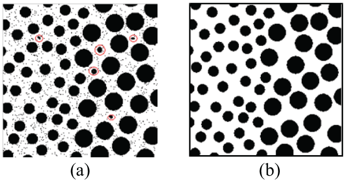
Binary image and connected region: (a) binary image with noise and (b) result of the noise removing.

Point cloud clustering based on SNCRL

Since there is not any topological structure in the point cloud, the neighborhood is very important for constructing the connected region. The most commonly used neighborhood in point cloud processing is the k-nearest neighborhood (kNN). It is defined as follows. Given a point cloud P of n points in IR^d and a positive integer $k\le n-1$ , the kNN of each point in P is computed. More formally, let P = {p₁, p₂,…, p_n} be a point cloud in IR^d, where $d\le 3$ ; for each $p_i\in P$ , let kNN(p_i) be the k points in P, closest to $p_i$ . kNN(p_i) = {q₁, q₂,…, q_k}. There are two methods to search the kNN for any point: the spatial partition algorithm and KD tree algorithm. ³⁰ We use the KD tree algorithm to search kNN. The KD tree algorithm divides a dataset into multi-level subspaces to build tree nodes that store the space range of partition data space into clipped super planes to reduce the searching scope. Therefore, it can efficiently search the kNN points. The spatial connectivity criterion is defined in the following.

Definition: spatial connectivity criterion. Given dataset P = {p₁, p₂,…, p_n}, n is the number of points. If p_i is the neighborhood of p_j, and p_j is also the neighborhood of p_i, then p_i and p_j are connectivity or p_i and p_j are adjacent.

Adding the adjacent points to one cluster according to the spatial connectivity criterion, the point in one cluster forms a connected region. The SNCRL algorithm can be summarized as follows:

1. Constructing kNN based on the KD tree for the input dataset.

2. Traversing the dataset to add current point p_i to current cluster C_{current_cluster}.

3. Checking the connectivity of p_i with kNN(p_i) according to the spatial connectivity criterion.

4. If p_i and q_j are connectivity, then checking whether q_j is added to other connected region C_{used_cluster}. If it is, then points in C_{current_cluste} and C_{used_cluster} clusters are from a connected region, and merging them to form one cluster, Otherwise, adding q_j to the current connected region C_{current_cluste}.

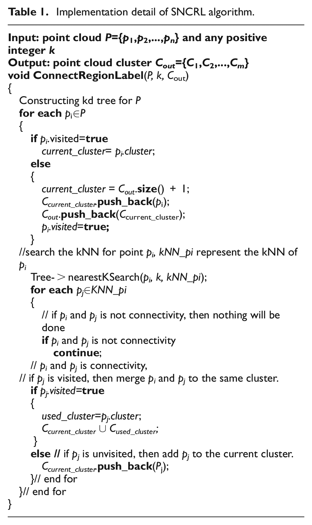
The implementation details of SNCRL are shown in Table 1.

Table 1.

Implementation detail of SNCRL algorithm.

Input: point cloud P={p1,p2,…,pn} and any positive integer k Output: point cloud cluster Cout={C1,C2,…,Cm}

void ConnectRegionLabel(P, k, Cout){ Constructing kd tree for P for eachpi∈P {  ifpi.visited=true   current_cluster= pi.cluster;  else  {   current_cluster = Cout.size() + 1;   Ccurrent_cluster.push_back(pi);   Cout.push_back(Ccurrent_cluster);   pi.visited=true;  } //search the kNN for point pi, kNN_pi represent the kNN of pi  Tree->nearestKSearch(pi, k, kNN_pi);  for eachpj∈KNN_pi  {   // if pi and pj is not connectivity, then nothing will be done   ifpi and pj is not connectivity    continue;  // pi and pj is connectivity, // if pj is visited, then merge pi and pj to the same cluster.  ifpj.visited= true  {   used_cluster=pj.cluster;   Ccurrent_cluster∪Cused_cluster;   }  else // if pj is unvisited, then add pj to the current cluster.   Ccurrent_cluster.push_back(Pj);  }// end for }// end for}

It should be noted that different k would construct different k-connectivity and connected regions. If k is set as a too large value, some small clusters closing to the large cluster would be classified into the large cluster. Therefore, the small cluster which may be outlier cluster is ignored. Figure 2 shows the clustering results for the point cloud based on different k-connectivity. Figure 2(a) displays the point cloud which consists of C₁, C₂, C₃ and C₄ clusters, where C₃ and C₄ are two small clusters. C₁, C₂, C₃ and C₄ are represented with white, green, blue and purple color, respectively. When k = 4, four clusters are classified correctly, as shown in Figure 2(b). When k = 12, the small cluster C₄ is classified into C₁, and when k = 32, both small clusters C₃ and C₄ are classified into C₁. The clustering results are shown in Figure 2(c) and (d), the point in the same color represents one cluster. In a practical application, the value of k can be determined according to the number of point clouds and size of outlier cluster. If the outlier cluster is relatively small, the value of k can be set to 4–6. When the point cloud model contains a large number of data and the outlier cluster is large, k can be set to 8–32 as reference.

Figure 2.

Point cloud connected region labeling results based on different k-connectivity: (a) point cloud; (b)–(d) connected region labeling results based on k = 4, 12, 32, respectively.

Experimental results and analysis

Comprehensive experiments were conducted on both synthetic and real datasets to assess the accuracy and efficiency of the proposed approach. Our experiments were run on a PC with Intel Core 2.30 GHz CPU, 16 GB memory. Experiments were conducted on point cloud clustering and outlier detection for different datasets.

Data clustering and comparison

In order to verify the effectiveness of the proposed method, both synthetic and real-world datasets were used in the performance evaluation. In the experiment, we compared our method with three state-of-art clustering approaches, including K-means clustering, ⁶ hierarchical clustering ²¹ and DBSCAN methods. ⁵ We implemented our method using Visual Studio 2017, with C++ language based on PCL 1.9 library. Other clustering algorithms are implemented in MATLAB 2014a; implementations of K-means clustering and hierarchical clustering algorithms are encapsulated in the toolbox of MATLAB.

We first conducted comparison experiments based on three synthetic datasets. Figure 3(a)–(c) shows three original datasets D₁, D₂ and D₃, respectively. Point cloud in D₁ is regular distribution containing four clusters. D₂ and D₃ are irregular distributions containing four and three clusters, respectively. Points in one cluster are represented with one color. We also conducted comparison experiments on two real-world point cloud datasets. Figure 4(d) and (e) shows two original datasets D₄ and D₅. D₄ is the point cloud of a drill; taken from the Stanford 3D Scanning Repository, ³¹ its file name is drill_1.6mm_270_cyb. D₄ contains 4294 points including seven clusters. Point cloud dataset D₅ is a car model, collected by a hand-type laser scanner. D₅ not only contains the car points, but also the background. D₅ contains two clusters: one is the car point cloud and the other is background. The original dataset contains more than 300,000 points, but it is downsampled to 53,604 points for test considering time-saving for large datasets. D₅ is wrapped for display.

Figure 3.

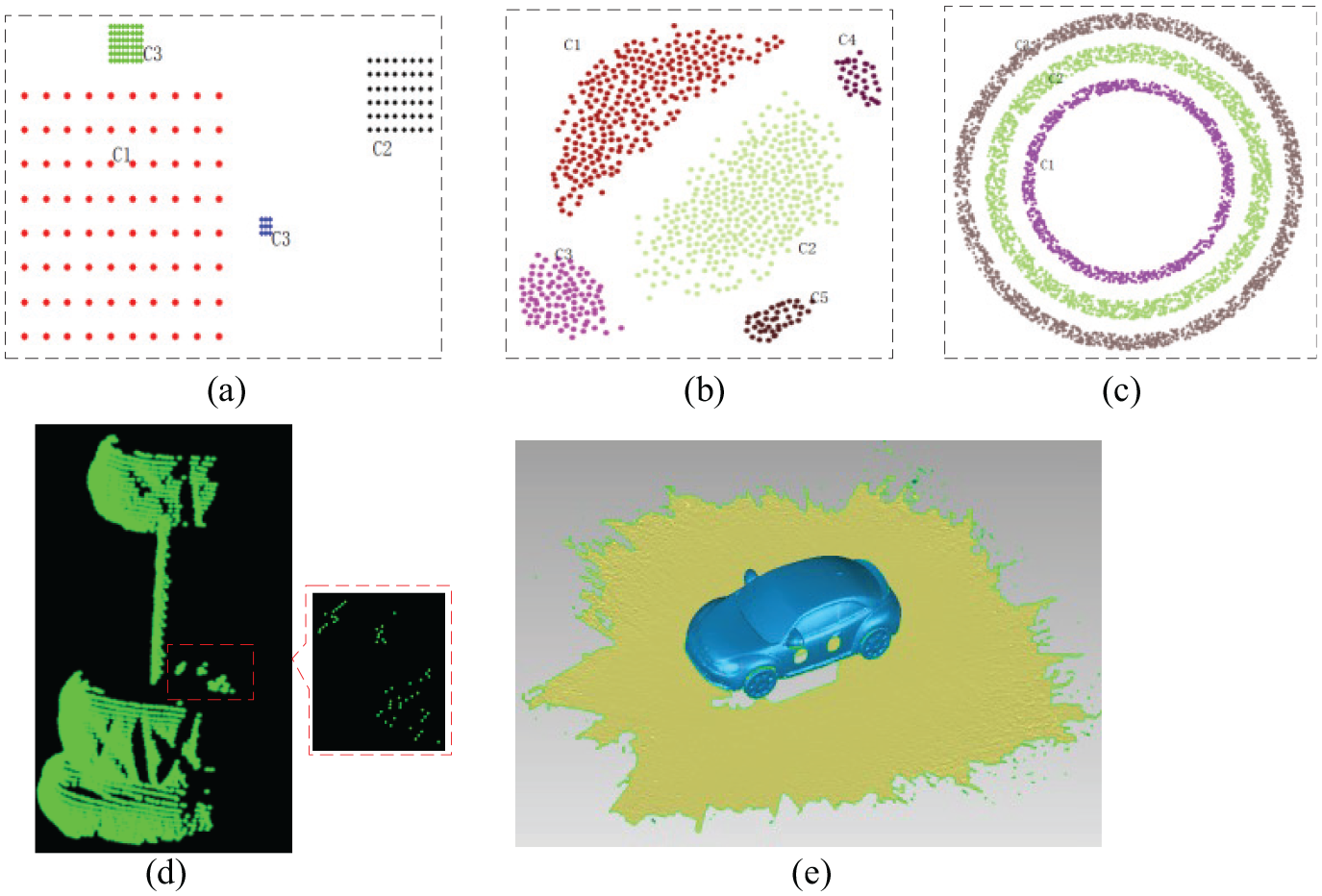
Test datasets: (a)–(e) is D₁–D₅, respectively.

Figure 4.

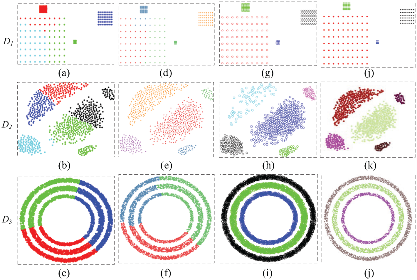
Clustering results for D₁, D₂ and D₃ based on K-means, hierarchical, DBSCAN and our method: (a)–(c) are results based on K-means algorithm; (d)–(f) are results based on hierarchical algorithm; (g)–(i) are results based on DBSCAN algorithm; (j)–(l) are results based on our method.

The clustering results of four algorithms for five datasets are shown in Figures 4 and 5. Each cluster is represented with one color. Each method has some key parameters. These parameters are very important to ensure clustering results correctly. The parameters of each clustering algorithm and elapsed time for five datasets are shown in Table 2.

Figure 5.

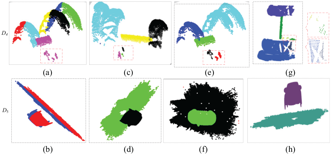
Clustering results for real-world datasets D₄ and D₅: (a) and (b) are results based on K-means algorithm; (c) and (d) are results based on hierarchical algorithm; (e) and (f) are results based on DBSCAN algorithm; (g) and (h) are results based on our method.

Table 2.

Parameter setting and time-consuming for four algorithms.

Dataset	Point numb	Time-consuming (s)
		K-means (iteration:6)	Hierarchical	DBSCAN	Our method
D 1	185	0.145 (K = 4)	0.271	0.048 (k = 6)	0.000 (k = 6)
D 2	765	0.516 (K = 5)	2.061	0.084 (k = 10)	0.001 (k = 10)
D 3	5000	0.205 (K = 3)	3.996	1.105 (k = 10)	0.031 (k = 10)
D 4	4294	0.248 (K = 7)	2.983	0.828 (k = 10	0.015 (k = 10)
D 5	53,604	0.181 (K = 2)	300.87	229.507 (k = 10)	0.297 (k = 10)

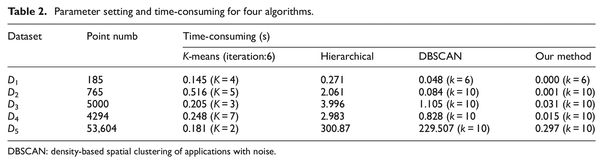
DBSCAN: density-based spatial clustering of applications with noise.

From the experimental results of synthetic datasets, K-means classify three datasets incorrectly. Hierarchical clustering algorithm categories D₂ correctly but incorrectly classify the other two datasets. DBSCAN and our method classify three datasets correctly. Figure 5 is clustering results for real-world datasets. Since clustering methods of K-means, hierarchical clustering, DBSCAN are implemented in MATLAB, the view of display is different from our method which is implemented in Visual Studio based on PCL. Hierarchical clustering and DBSCAN methods can classify most of the clusters correctly for D₄ and D₅, only a few points are divided by mistake. For example, there are three small clusters in D₄, shown as red rectangular area in Figure 3(d), but the DBSCAN algorithm classifies these three clusters into two clusters; clustering result is shown in Figure 5(e). Our method accurately divides all points into the right clusters for D₄ and D₅.

Time and computational complexity analysis

For n points, the computational complexity of K-means is K × n × N × i as discussed in section “Introduction.” Generally, the complexity of hierarchical clustering is O(n³). ¹ The computation complexity of DBSCAN is O(n log(n)) based on KD tree searching. ¹ Our method includes constructing the KD tree, searching every point and querying its neighborhood. The total computation complexity of our method is about O(log₂ n) + O(kn), where k is the neighborhood size. It can be seen that these clustering algorithms are very complex and time-consuming in the application of large amount of data. The execution times of four methods for five datasets are shown in Table 2. Different compilers may take different times to implement the same algorithm; therefore, the elapsed time for four algorithms listed in Table 2 is just for reference, not for comparison. The time-consuming can be known according to the algorithm complexity.

Outlier detection for point cloud

In order to test the effectiveness of our method for the point cloud outlier detection, synthetic datasets are employed for quantifying results. Real-world datasets including the outdoor and indoor collected point cloud are also tested to verify the effectiveness.

Outlier detection and performance for the synthetic dataset

Outlier detection rate (ODR), inlier detection rate (IDR), false positive rate (FPR) and false negative rate (FNR) and accuracy are employed to measure detection results, respectively. ¹⁶ ODR, IDR, FPR, FNR and Accuracy are defined as follows

$$\mathrm{ODR}=\frac{\mathrm{number}\mathrm{of}\mathrm{outliers}\mathrm{correctly}\mathrm{identified}}{\mathrm{total}\mathrm{number}\mathrm{of}\mathrm{outliers}}$$

(1)

$$\mathrm{IDR}=\frac{\mathrm{number}\mathrm{of}\mathrm{inliers}\mathrm{correctly}\mathrm{identified}}{\mathrm{total}\mathrm{number}\mathrm{of}\mathrm{inliers}}$$

(2)

$$\mathrm{FPR}=\frac{\mathrm{number}\mathrm{of}\mathrm{inliers}\mathrm{identified}\mathrm{as}\mathrm{outliers}}{\mathrm{total}\mathrm{number}\mathrm{of}\mathrm{inliers}}$$

(3)

$$\mathrm{FNR}=\frac{\mathrm{number}\mathrm{of}\mathrm{outliers}\mathrm{identified}\mathrm{as}\mathrm{inliers}}{\mathrm{total}\mathrm{number}\mathrm{of}\mathrm{outliers}}$$

(4)

$$\mathrm{Accuracy}=\frac{\mathrm{TP}+\mathrm{TN}}{\mathrm{total}\mathrm{number}\mathrm{of}\mathrm{points}}$$

(5)

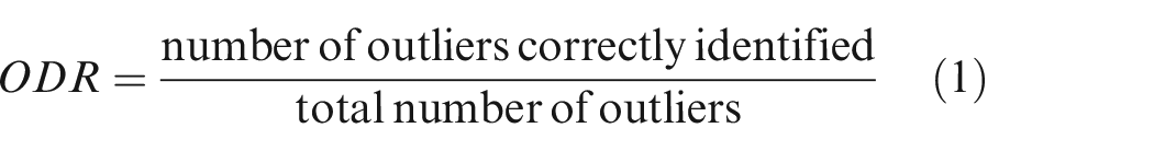
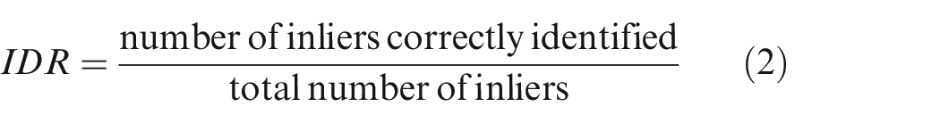
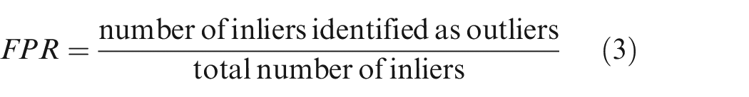
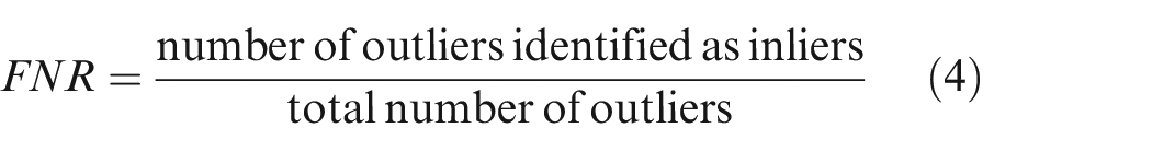
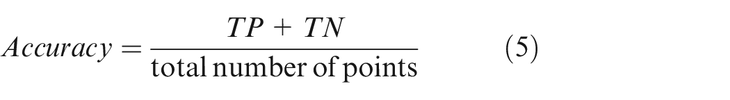
where TP and TN represent the number of correctly identified outliers and inliers, respectively. The maximum value of IDR, ODR, FPR, FNR and Accuracy is 1, and their minimum values are 0. The bigger the value of IDR, IDR and Accuracy is, and the smaller the value of FPR and FNR is, the better result of the outlier detection is.

In order to accurately quantify outlier detection results, synthetic datasets D₆, D₇ and D₈ with different outliers are employed to verify the effectiveness of our algorithm. D₆ contains 166 points including 34 outliers and 132 inliers. D₇ contains 603 points including 60 outliers and 543 inliers. D₈ contains 5180 points including 180 outliers and 5000 inliers. Inliers in D₆ are the regular distribution, but irregular distributions in D₇ and D₈. Each dataset contains sparse outliers and cluster outliers, and some sparse outliers are closed to the normal data. Outliers in D₆, D₇ and D₈ are added manually using the Geomagic software. The outliers are represented with red dot points shown in Figure 6(a)–(c). The state-of-art outlier detection methods such as LOF, DBSCAN algorithms are compared to our method. The outlier detection results for LOF, DBSCAN and our method are shown in Figure 6, where the red symbol “+” represents the identified outliers. It shows that the LOF method can identify most of the sparse outliers but identify cluster outliers as inliers by mistake. The DBSCAN method can detect most of the sparse and cluster outliers, but identify some outliers that are close to normal points as inliers by mistake. Our method identifies most of the outliers including sparse and cluster outliers, but wrongly classifies a few outliers that are very close to normal points to inliers, as shown in Figure 6(j) and (l).

Figure 6.

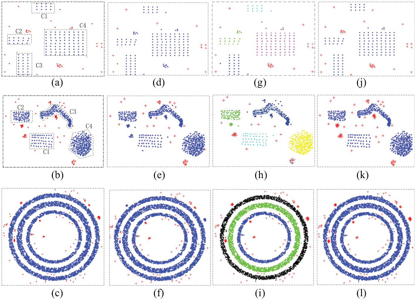
Outlier detection results for synthetic datasets: (a)–(c) is outliers of D₆, D₇ and D₈ with red dot points, respectively; (d)–(f) are outlier detection results using the LOF method; (g)–(i) are outlier detection results using the DBSCAN method; (j)–(l) are outlier detection results using our method.

Tables 3–5 show the values of ODR, IDR, FPR, FNR and Accuracy for three synthetic datasets. It can be seen from these tables that values of ODR, IDR and Accuracy are close to 1, and values of FPR and FNR are close to 0. Outlier detection results based on our method is better than LOF and DBSCAN methods.

Table 3.

Measurement results based on the LOF method.

Dataset	Parameter		Result
	k	Threshold	ODR	IDR	FPR	FNR	Accuracy
D 1	6	1.5	0.353	1	0.002	0.647	0.867
D 2	6	1.5	0.5	1	0	0.55	0.94
D 3	8	1.5	0.538	0.998	0.002	0.4625	0.986

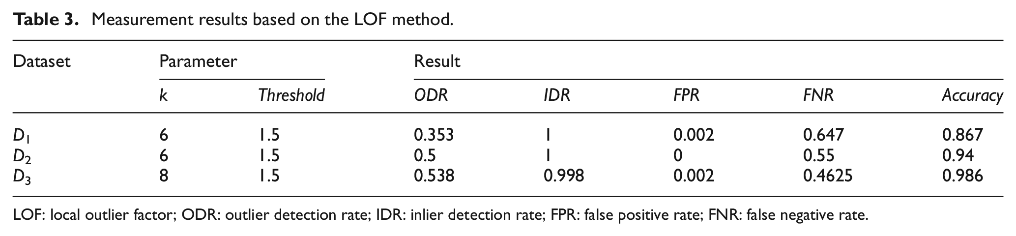
LOF: local outlier factor; ODR: outlier detection rate; IDR: inlier detection rate; FPR: false positive rate; FNR: false negative rate.

Table 4.

Measurement results based on the DBSCAN method.

Dataset	Parameter		Result
	k	Threshold	ODR	IDR	FPR	FNR	Accuracy
D 1	6	10	0.467	1	0	0.583	0.947
D 2	6	15	0.559	1	0	0.441	0.307
D 3	6	100	0.635	1	0	0.365	0.997

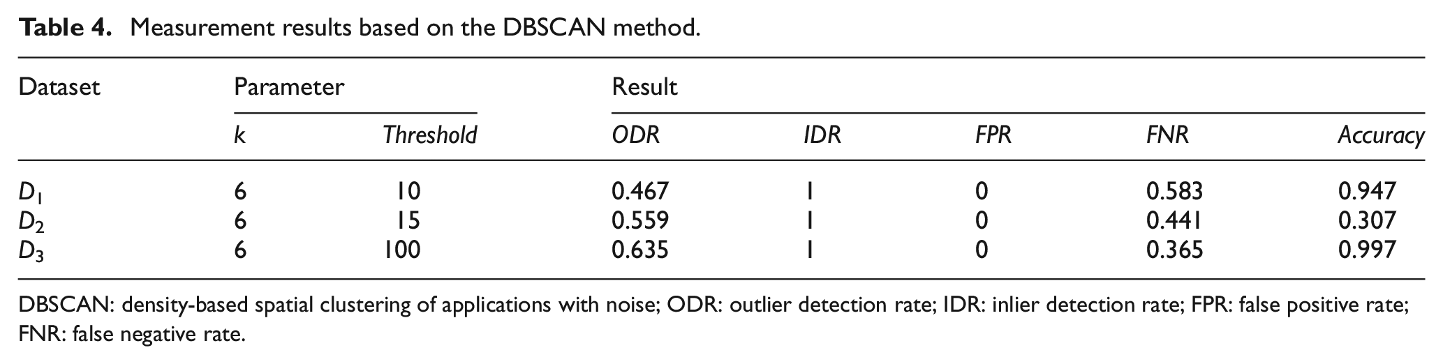
DBSCAN: density-based spatial clustering of applications with noise; ODR: outlier detection rate; IDR: inlier detection rate; FPR: false positive rate; FNR: false negative rate.

Table 5.

Measurement results based on our method.

Dataset	Parameter		Result
	k	Threshold	ODR	IDR	FPR	FNR	Accuracy
D 1	4	10	0.882	1	0	0.133	0.976
D 2	4	15	1	1	0	0	1
D 3	8	100	0.916	1	0	0.084	0.999

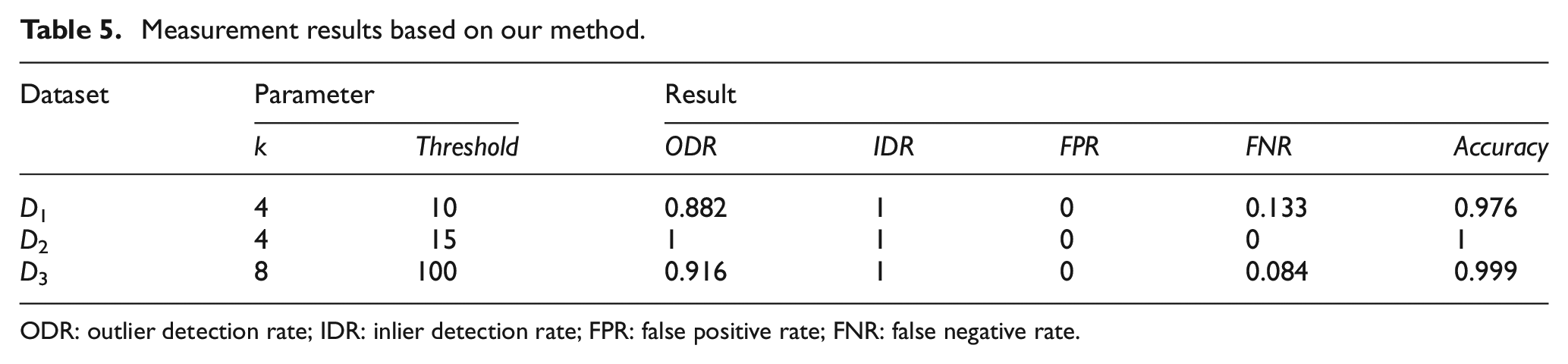
ODR: outlier detection rate; IDR: inlier detection rate; FPR: false positive rate; FNR: false negative rate.

Outlier detection for real-world three-dimensional point cloud

Two real-world datasets D₉ and D₁₀ are tested for the outlier detection. D₉ is the point cloud of railway acquired by a hard-type laser scanner. D₁₀ is the point cloud of Happy Buddha from the Stanford 3D Scanning Repository. Affected by the environment, equipment and shape of the measured object, the scanned point cloud data are composed of a series of clusters or sparse outliers usually. Since the real-world dataset contains a mass of points, it is difficult to know the number of outliers accurately and there is no ground-truth for the noiseless point cloud. Therefore, we do not quantitatively compare the outlier detection results for these datasets. D₉ and D₁₀ consist of many clusters, and some clusters are outlier clusters. The point cloud with outliers would affect the result of point processing; thus, it is necessary to remove outliers before data processing in the point cloud registration and surface reconstruction. Since it is difficult to accurately calculate all the clusters and sparse outliers manually, we manually select some small clusters that are outlier clusters to test the outlier detection results of different algorithms. We select 14 clusters and 9 clusters that containing points less than 100 for D₉ and D₁₀, respectively. Our method identifies all clusters for both datasets, and the clustering and outlier detection results are shown in Figures 7 and 8 where one color represents one cluster. The DBSCAN method only identifies six clusters and five clusters for D₉ and D₁₀, respectively, and the result can be seen in Figure 9(a) and (b). The LOF method detects some boundary points and some points with a large density to outliers, and the outlier detection results are shown in Figure 9(c) and (d), where red points represent outliers.

Figure 7.

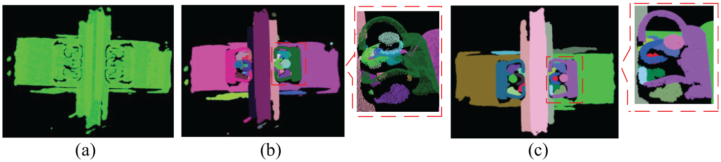
Data clustering and outlier remover for railway point cloud: (a)–(c) is the original point cloud, data clustering result based on our method and the result of removing small cluster, respectively.

Figure 8.

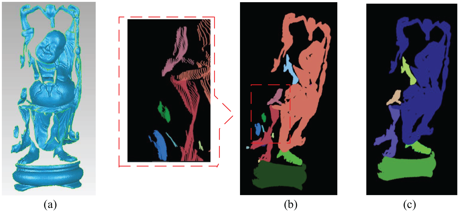
Data clustering and outlier remover for Happy Buddha point cloud: (a)–(c) is the original point cloud, data clustering result based on our method and the result of removing small cluster, respectively.

Figure 9.

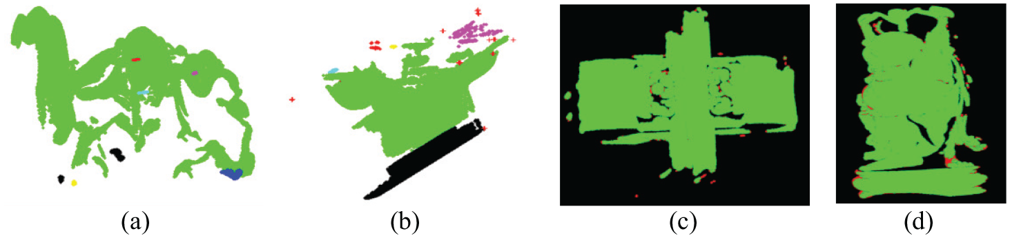
Outlier detection result for D₉ and D₁₀: (a) and (b) is the outlier detection result of D₉ and D₁₀ based on DBSCAN method, respectively; (c) and (d) is the outlier detection result of D₉ and D₁₀ based on LOF method, respectively.

Conclusion

In this paper, a novel data clustering and outlier detection approach, called SNCRL, is presented. The data points are categorized into different clusters according to the connectivity criterion. The method can effectively and efficiently classify data into appropriate clusters and identify outliers for point cloud datasets. Comparing with the K-means, hierarchical clustering and DBSCAN methods, our method is less computation complexity and less time-consuming for data clustering. In addition, our method requires only one parameter k to be set for the size of neighborhood. Our method can not only detect cluster outliers, but also sparse outliers. For applications of the point cloud outlier detection, our method can identify outliers more accurately compared to LOF and DBSCAN algorithms.