Sage Journals: Discover world-class research

Abstract

Cantilever beams can have various behaviour depending on the details of the connection. Partially-fixed connections have a different performance from conventionally-fixed connections, in which the exact information is not available. In this paper, using the finite element model updating (FEMU) of a steel cantilever beam, the support conditions of a partially-fixed connection and the behaviour of the beam are investigated. The FEMU is utilized as an appropriate technique for structural health monitoring, which requires the use of data acquisition methods from the structure. In this research, instead of using discrete sensors, displacement and strain information are continuously measured from the beam surface using the digital image correlation (DIC) method. The difference between the initial model and the data extracted from the DIC is determined by a cost function. A hybrid method called Powell particle swarm optimization is used to minimize the cost function. This method includes particle swarm optimization (PSO) as a global search technique and Powell optimization as a local search technique; the hybrid method achieves better performance by combining the two methods. A dynamic inertia weight is presented to improve the performance of the PSO algorithm. Abaqus software and Python programming have been used to carry out the FEMU process. Finally, the amount of rotation and displacement of support are calculated, and the dependency of beam behaviour on each of the variables is investigated. This method yields acceptable convergence of the results and can be extended to study other structural components.

Keywords

Finite element model updating structural health monitoring digital image correlation particle swarm optimization Powell optimization hybrid swarm optimization

Introduction

Cantilever beams are one of the different types of structural members that have different applications in buildings, bridges, etc. In some research, the behaviour of these beams under the influence of different conditions has been studied.^1,2 In cantilever beams, connections are of great importance, so various studies have been performed regarding the repair of damaged welded connections,³ the use of precast post-tensioned connections,⁴ etc. There are different kinds of connections, such as fixed connections, partially-fixed connections, etc., which fixed connection is commonly used in the design of cantilever beams. The behaviour of partially-fixed connections is different from fixed connections; therefore, different studies have been conducted specifically on partially-fixed connections.^5–7 In this research, a partially-fixed connection has been utilized to investigate the performance of the presented finite element model updating (FEMU) process. Connections can affect the behaviour of the beam based on their rigidity and influence the amount of displacement and strain of the beam. In connections with inadequate information, such as in old structures and not maintaining the initial performance due to various reasons such as corrosion, and in relatively new connections lacking boundary information, it is required to ensure their performance according to the existing conditions.

Investigating the behaviour of structural members and identifying their performance under different conditions provide the possibility of monitoring the health of the structure. Structures undergo different kinds of deterioration over time, and structural health monitoring (SHM) allows the owner or the operator to have a good understanding of the structural condition and its effect on remaining service-life and capacity.⁸ In recent years, new approaches have been proposed to improve the SHM process, using a variety of techniques including machine learning techniques,^9,10 signal processing techniques,¹¹ image processing techniques,^12,13 etc.

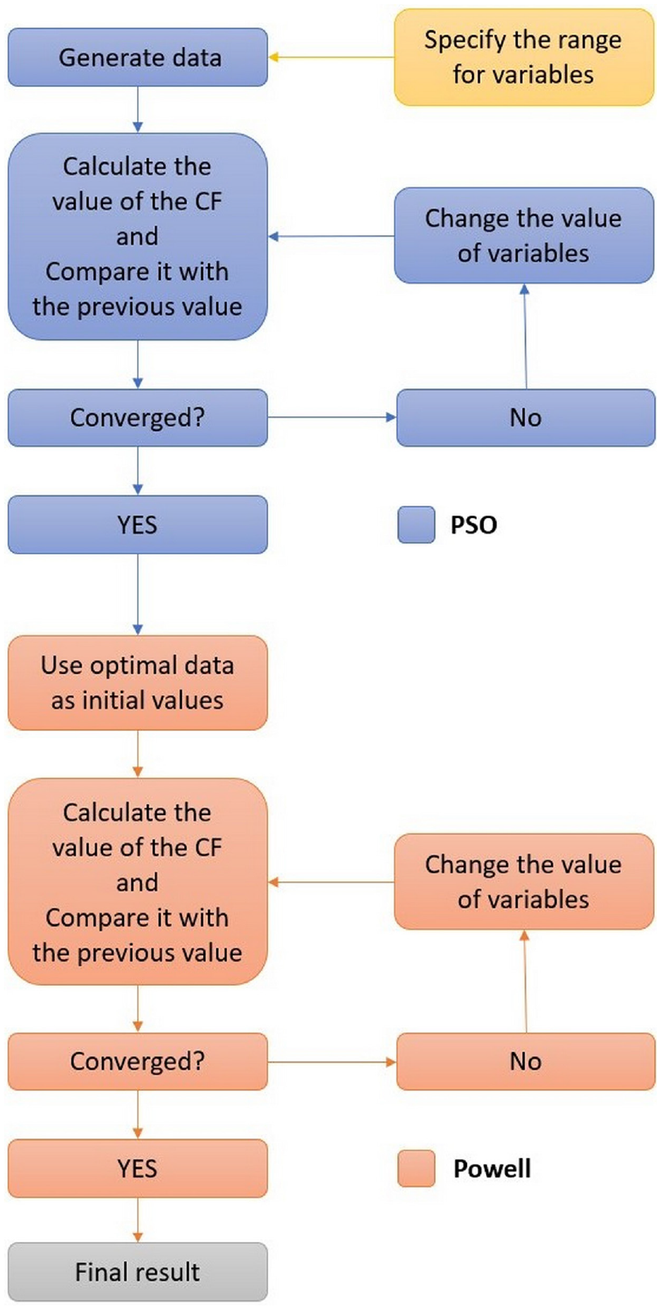
One of the challenges in engineering structures is evaluating the performance of structures based on their current condition and finding differences between numerical models and experimental observations. While the finite element method is commonly used to study the behaviour of structures,^14–16 the FEMU method is one of the most widely used methods in the literature by which the initial model is updated according to the observed data to minimize the difference between the existing structure and the numerical simulation.^17–20 Therefore, it is very useful in SHM and damage detection systems.^21–23 An overview of the FEMU process steps in the present research is shown in Figure 1.

Figure 1.

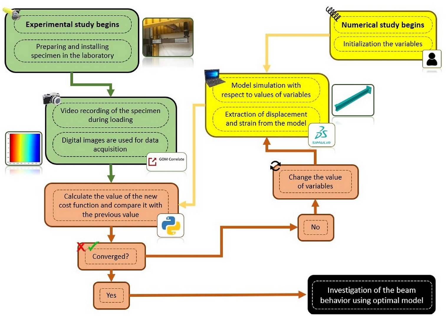
An overview of the FEMU process steps in the present research.

FEMU is widely classified into two categories: direct methods and iterative methods. Most of the early proposed models are in the category of direct methods.²⁴ The direct methods are a one-step method that directly updates stiffness and mass matrices. Although direct methods have been used in many cases,^25–27 iterative methods, such as sensitivity-based methods²⁸ and dynamic perturbation method,²⁹ are more popular because of their ease of implementation.³⁰ In this method, the error between the experimental data and the initial model is determined using an objective function, and then the function is minimized by different optimization methods to obtain the updated model with the least error, in a way that the optimal value of the finite element model (FEM) parameters is achieved. These parameters can include boundary conditions, density, Young’s Modulus, Poisson’s ratio, etc. Using this method can have important advantages. For instance, wide choices of updating parameters can be provided. In addition, the structural connectivity can be easily maintained, and the proposed modifications to the selected parameters can be physically interpreted.³¹

The FEMU method requires experimental observations that can be obtained using various data acquisition methods. In the past, data acquisition was done by installing physical sensors on a specimen that extracted the values discretely. However, the use of digital cameras makes it possible to use the digital image correlation (DIC) method to continuously obtain the desired values from the specimen and examine the structure without the need of installing physical sensors. DIC has a better performance compared to Linear Variable Differential Transformer (LVDT) sensors and strain gauges that can extract only values at a single point. The DIC method has gained significant popularity in recent years, and various studies have been performed using this technique,^32–37 as it can update the FEM in a more efficient way. The DIC method obtains the amount of displacement and strain of the desired surface by comparing the images taken from the specimen, before and after the deformation.³⁸ The first image taken from the specimen before loading is considered the reference image, and then the images taken during loading are compared with the reference image, and thus provide the values of displacement and strain at each moment. It should be noted that in other cases, such as crack propagation detection based on increasing crack width, this technique can also be used.³⁹

Optimization is the last step in the FEMU process. Different methods can be used to solve the optimization problem, which should be selected according to the type of problem. Optimization in the FEMU process usually has several local minima, so using local search techniques cannot achieve a global minimum.⁴⁰ Therefore, an appropriate method should be used in this type of problem. The hybrid method is one of the popular optimization methods for which various approaches have been presented.^41,42 In hybrid methods, a metaheuristic method obtains the optimal value of the objective function approximately, then this value is used as the initial estimated value by a local search technique to determine the optimal value accurately. Metaheuristic methods such as particle swarm optimization (PSO),⁴³ genetic algorithms⁴⁴ and simulated annealing⁴⁵ are usually stochastic in nature and improve a randomly generated set of initial designs in a pseudorandom fashion.⁴⁶

This paper investigates the behaviour of a steel cantilever beam with a partially-fixed connection by presenting a FEMU process based on DIC and Powell particle swarm optimization (PPSO). The purpose of presenting the FEMU process is to evaluate the behaviour of beams based on the connection behaviour regardless of the connection type and to reduce the error between the numerical model and the real sample. In the presented FEMU process, by using an improved optimization algorithm, the convergence speed has increased compared to the original algorithms; on the other hand, due to the use of the full field measurement technique along with the hybrid optimization algorithm, the accuracy of the optimal model has increased. Data acquisition from the beam surface is performed by the DIC method at the free end and support. Strain gauges and LVDT sensor are installed on the specimen to check the validity of the data extracted by the DIC method. Finally, using a cost function, the amount of error between the experimental data and the numerical model is determined, which is optimized using a hybrid method. The hybrid method consists of PSO, as a global search technique, and Powell optimization, as a local search technique, which can achieve better performance in finding the optimal value. PSO is a global optimization method for locating a deep local minimum among all local minima that is based on the behaviour of the birds in a swarm.^47,48 Powell is a gradient-free minimization algorithm that finds the most accurate minimum value near the starting point.⁴⁹ Finally, the appropriate performance of the FEMU process is confirmed and it is also found that the simulated rotational spring on the support has the greatest effect on the vertical displacement of the beam and the Young’s modulus has a great effect on the strain. It should be noted that the PPSO algorithm provides acceptable results.

Experimental study

To investigate the behaviour of a steel cantilever beam with a partially-fixed connection, an experimental study is provided along with a numerical model. The experimental study that includes fabrication and installation of specimen in the laboratory and data acquisition under loading is an important part of this research, because the accuracy and quality of the work will play a significant role in the results. In this section, the details of the specimen, loading, sensors and data acquisition method are presented.

Test setup

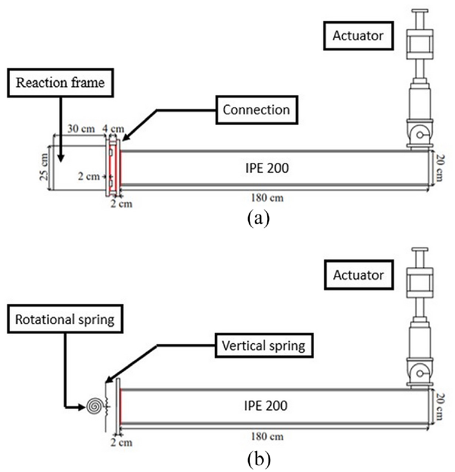
The test specimen is an IPE 200 steel beam (according to DIN 1025-5⁵⁰) with a length of 180 cm, without considering the connection. One end of the beam is connected to the laboratory’s reaction frame using a welded/bolted connection, and the other end is free. The total length of the beam, including the connection, is 188 cm. Additionally, loading is applied by an actuator to the free end. Figure 2 shows configuration of the beam after preparation and installation at the strong floor laboratory.

Figure 2.

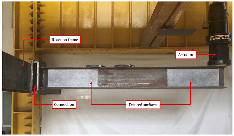
Test specimen and point loading at free end.

As the DIC method works based on the images taken from the specimen during loading, two parts of the beam surface are prepared for data acquisition. The first part is at the beginning of the beam, where the maximum strain occurs, and the second part is at the free end, where the maximum vertical displacement occurs. The desired surfaces for DIC are cleaned and made free of any grease or oil, and then are coated using white dull paint spray. Finally, after the white colour dries, a stochastic pattern using black dull paint spray is applied. These steps are performed, so that the desired surfaces can be detected well by the cameras.

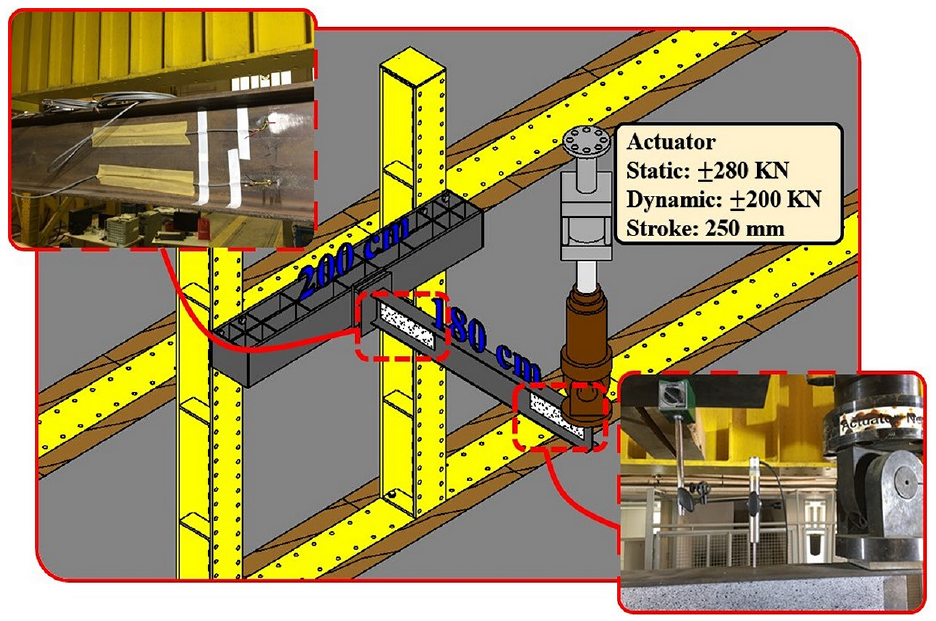
After completing the beam painting process and checking the quality of the patterns, the beam is welded to the connection according to the details provided in the next section. To confirm the results of the DIC method, two strain gauges at the support and one LVDT sensor at the free end have been used. The strain gauges are of FLA-5-11 type with a resistance of $120 \pm 0.3 Ω$ , which extracting the strain of the beam in its longitudinal direction in the desired points. Strain gauges are mounted at a distance of 30 cm from the support, and at the top and bottom of the designated web area with 12 and 40 cm width and height, respectively, the LVDT sensor is installed at a distance of 30 cm from the free end. The location of the sensors and actuator specifications are shown in Figure 3.

Figure 3.

The location of the sensors and actuator specifications.

End connection of beam

According to the conditions of the laboratory reaction frame, a welded/bolted connection is designed which is a partially-fixed connection that can be well connected to the laboratory frame. The connection consists of two plates with dimensions of 25 × 32 cm² with a thickness of 20 mm, which are connected using a heavy I-shaped cross section. The connection is made of ST52-3 grade steel. The first plate is connected to the laboratory frame using four M24 bolts, and the beam is welded to the middle of the second plate using continuous fillet weld. Figure 4 shows the details of the connection and the assembly steps, which includes three steps. In the first step, the elements are cut and first plate element drilled. In the second step, the I-shaped section is welded to the first plate and the bolts are inserted (due to the limited dimensions after welding). In the last step, the second plate is connected to the I-shaped element and the welding is completed. It should be noted that the location of the main beam on the second plate is specified, which will be welded after the connection is completed.

Figure 4.

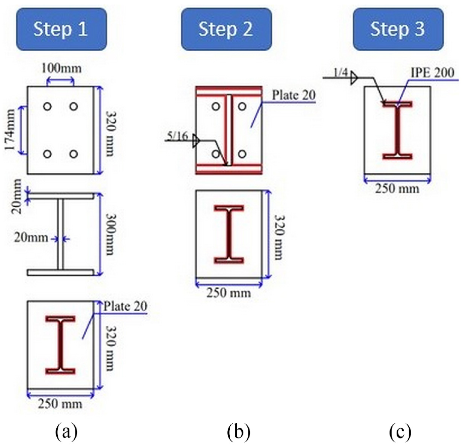
The details of the connection and the assembly steps: (a) Cut and drill, (b) I-section welding to the first plate, and (c) completion of the welding process.

Figure 5 shows the welding of connection elements. According to the dimensions considered for the connection components, its performance is assumed to be rigid. Therefore, the connection is simulated as a set of springs at the joint connection and its performance is investigated according to its effects on the beam. The use of springs in the supports allows the displacement and rotation of the support to be adjustable based on the actual behaviour of the connection.

Figure 5.

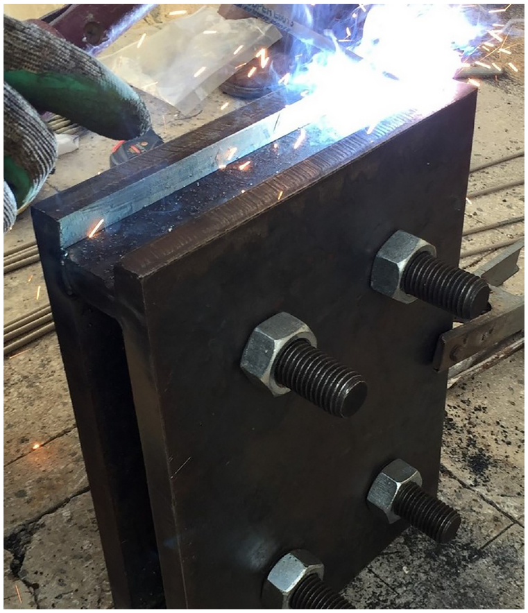
Welding of connection elements.

Loading

In this test, concentrated loading is applied at the free end of the beam. Under the actuator, a steel plate with dimensions of 10 × 10 cm² with a thickness of 20 mm is used to transfer the point load. The specimen is tested under displacement-controlled loading condition, which is applied as a half-sinusoidal load in 120 s. The maximum amount of displacement is 30 mm, which occurs in the 60 s. The amount of displacement applied to the beam should be determined based on the connection conditions. If a fully-fixed connection was used in this experiment, the beam would enter the plastic region at a displacement of 30 mm, but in here the beam remains in the elastic region due to the partially-fixed connection. For this reason, before conducting the main test, the maximum displacement of the actuator was determined with the help of strain gauges so that the beam does not enter the plastic region. The amount of actuator displacement is expressed as:

\begin{array}{l} y (t) = y_{\max} \sin (ω t) \\ y_{\max} = 30 mm, ω = π / 120 \\ y (t) = 30 \sin (π t / 120), 0 \leq t \leq 120 \end{array}

(1)

where y is the actuator displacement, t is the time, $y_{max}$ is the maximum displacement of the actuator and $ω$ is the angular frequency.

Digital image correlation

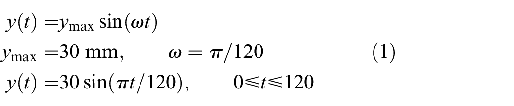
DIC is utilized as a powerful data acquisition method in this research. Figure 6 shows a comparison between the displacement values obtained by DIC method at the free end under various loading. As can be seen, the DIC measurements have been performed at the surface continuously.

Figure 6.

Displacement of the beam at (a) 0 s, (b) 40 s (loading), (c) 60 s (maximum loading) and (d) 80 s (unloading).

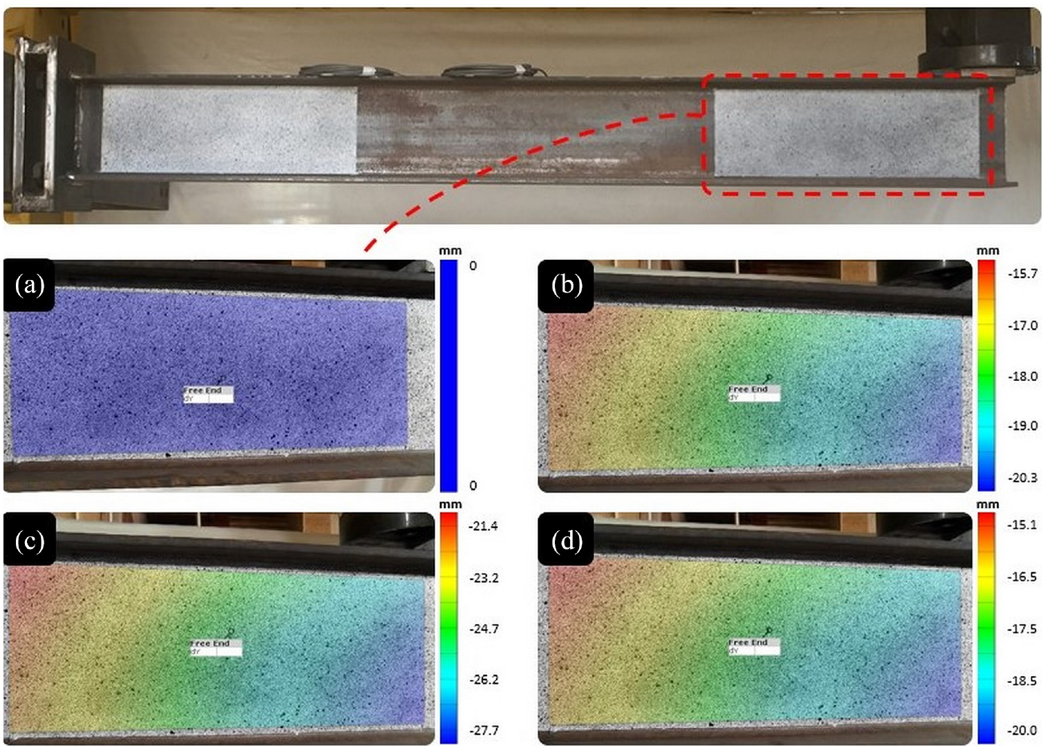
Two parts of the beam web are prepared for this work, the dimensions are 50 × 16 cm², and the exact position is shown in Figure 7(a). These two areas are recorded during loading and unloading, then each video is converted into several images so there will be one image per second. The prepared images are analysed using GOM Correlate software,⁵¹ and the amount of displacement and strain is extracted in each image or per second. Before performing the main test, the quality of the patterns is checked, because the quality of these patterns, in addition to the painting, is also very dependent on the ambient light. Figure 7(b) and (c) show the quality of the patterns. The quality of the pattern at the support is a little better than the free end, but in general, both are of good quality and acceptable.

Figure 7.

(a) Position and dimensions of the desired surfaces for data acquisition using the DIC method, (b) pattern quality at the support and (c) pattern quality at the free end.

The captured images by the cameras are 1920 × 1080 pixels. The image sensor is 1/4.1″ 1MOS. The focal length of the camera lens is 3.02 to 75.5 mm, which is set to 3.02 mm here, and the distance between the cameras and the beam is determined accordingly. The distance of the cameras from the beam is approximately 50 cm. Figure 8 shows the arrangement of DIC system in front of the specimen.

Figure 8.

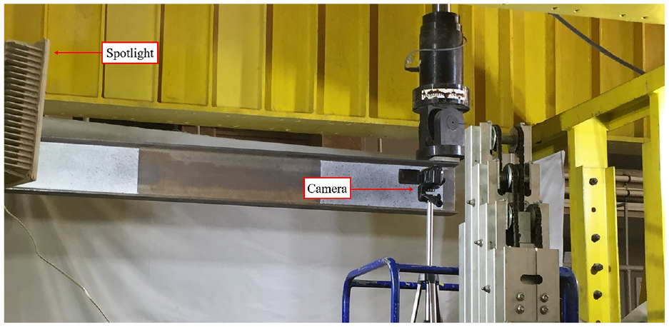
The arrangement of DIC system in front of the specimen.

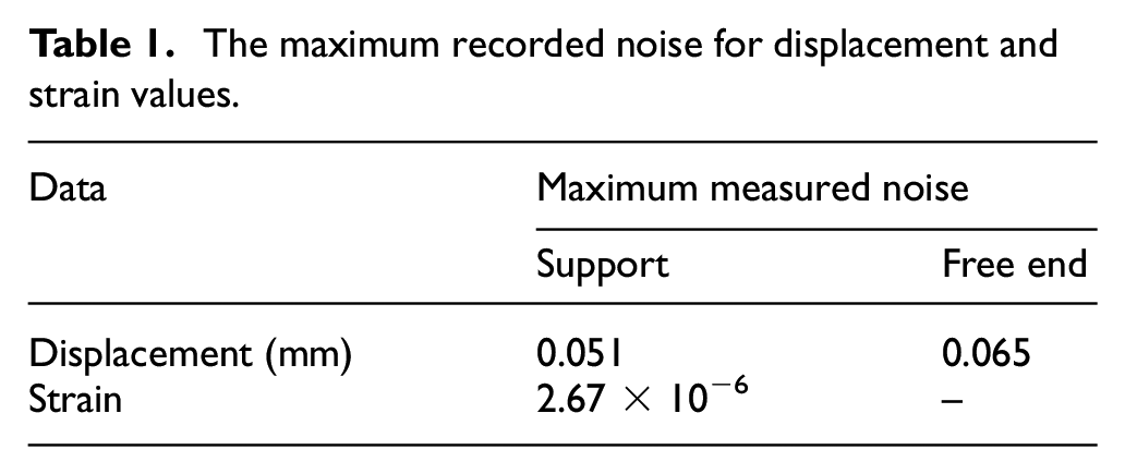
In the strong floor laboratory, there are various sources that can generate noise. Noise can influence the data, especially strain, so measuring noise is important. To measure noise, the specimen was recorded for 3 s before loading. After analysing the images, it was observed that the values of strain and displacement were not zero, which are called measurement errors. The average of the errors obtained per second are calculated and then subtracted from the main values. The maximum recorded noise for each of the displacement and strain values is presented in Table 1.

Table 1.

The maximum recorded noise for displacement and strain values.

Data	Maximum measured noise
Data	Support	Free end
Displacement (mm)	0.051	0.065
Strain	2.67 × 10⁻⁶	–

Numerical study

In this section, the objective and detailed FEMs are introduced. The initial objective model, after the optimization process, becomes an optimal model that has a high ability to investigate the behaviour of the specimen. Before starting the optimization process by defining a cost function, the error between the experimental observations and the numerical data is calculated. By minimizing the value of the cost function, the variables of the FEM are determined in such a way that the optimal model is obtained. Finally, in order to minimize the cost function, an optimization process is defined, which results in the lowest value of the cost function using a hybrid method.

Finite element model

The finite element method is an appropriate technique for numerical study of structures, only the initial FEM does not have high accuracy in evaluating the behaviour of the specimen, which requires updating the model by optimizing the variables that have the most influence on the behaviour of the model. Here, by presenting the objective FEM and defining model variables, it is possible to optimize the initial model based on experimental observations. In the objective FEM, the connection behaviour is simulated by vertical and rotational springs, and then the results are compared with a detailed FEM, which includes the simulation of the reaction frame, connection, bolts and weld. Figure 9 shows an overview of the detailed and objective FEMs.

Figure 9.

Overview of the (a) detailed and (b) objective finite element models.

In this study, the objective FEM is simulated in the Abaqus software, which includes 20,094 nodes and 11,760 linear brick elements. In order to update the model, several variables are considered, so that the optimal model will be achieved after determining the optimized value of the selected variables. The Young’s modulus (E_s), stiffness of the vertical spring (K₁) and stiffness of the rotational spring (K₂) are defined as variables. To optimize the objective FEM based on the strain data, Young’s modulus is considered as a variable, because it has a direct effect on the strain values of the beam. Young’s modulus is a fundamental property of materials and its value can be changed in a certain range and affects the behaviour of the structure. Cantilever beams that are made with a fixed connection do not have any rotation or displacement at the support, while for a partially-fixed support, there is a possibility of displacement and rotation. Therefore, a rotational spring is used to measure the amount of rotation and a vertical spring is used to measure the amount of vertical displacement. The vertical and rotational stiffness of the springs controls the amount of displacement and rotation of the support based on condition of the connection. The use of springs to simulate the behaviour of connection also identifies the differences and errors that may occur during the fabrication and installation of the connections. Due to the high dependence between behaviour of the support and behaviour of the beam, the stiffness of the springs has a great effect on behaviour of the beam. Density and Poisson’s ratio, which are other properties of the material, are assumed to be constant with a density of 7850 kg/m³ and a Poisson’s ratio of 0.28. Density and Poisson’s ratio can be among the variables, but they are considered here as constants in the objective FEM due to the conditions of the problem which is less dependent on these two parameters. Also, the dimensions of the FEM are considered based on the specimen and details provided in the previous section, which are constant during the optimization process. Figure 10 shows a view of the objective FEM of the beam.

Figure 10.

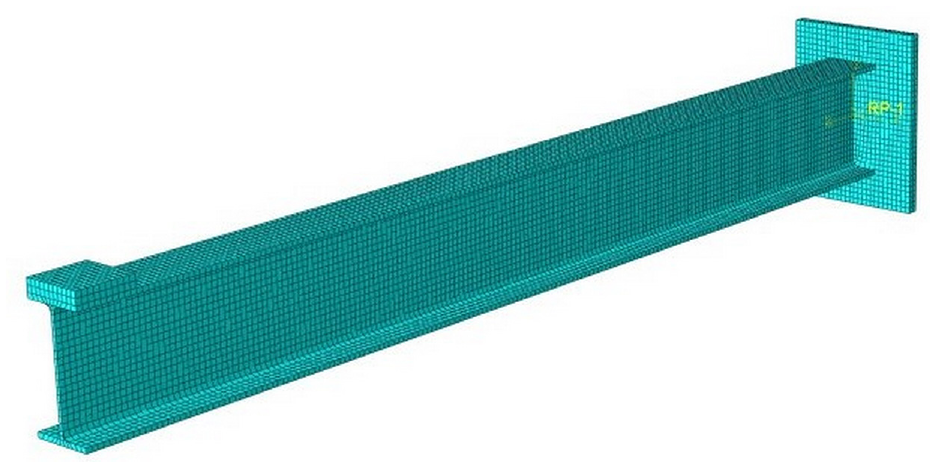
A view of the objective finite element model of the beam.

Theory of the objective FEM

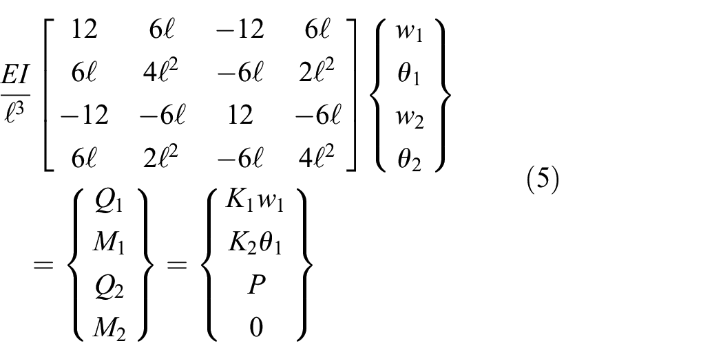
Figure 11 shows the theoretical view of the objective FEM, which is a beam with four degrees of freedom, and the element stiffness matrix is obtained using the following equation.⁵²

k_{e} = \int_{v} B^{T} cB d V

(2)

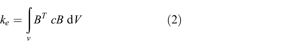
where B is the strain matrix and c is the matrix of material constants. By substituting $B = - yLN$ in this equation, the element stiffness matrix is written as follows.

\begin{matrix} k_{e} = \int_{v} B^{T} cB d V = E \int_{A} y^{2} d A \int_{0}^{ℓ} {(\frac{\partial^{2}}{\partial x^{2}} N)}^{T} (\frac{\partial^{2}}{\partial x^{2}} N) \\ d x = EI \int_{0}^{ℓ} {(N ″)}^{T} N ″ d x \end{matrix}

(3)

where L is a matrix of partial differential operators and N is a matrix of shape functions.

Figure 11.

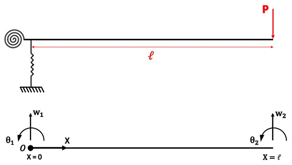
Theoretical view of the objective finite element model.

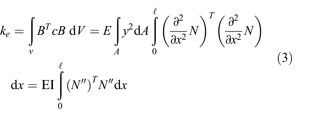
By obtaining N for the desired beam and substituting in the above equation, the stiffness matrix is obtained as follows.

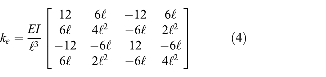
k_{e} = \frac{EI}{ℓ^{3}} [\begin{matrix} 12 & 6 ℓ & - 12 & 6 ℓ \\ 6 ℓ & 4 ℓ^{2} & - 6 ℓ & 2 ℓ^{2} \\ - 12 & - 6 ℓ & 12 & - 6 ℓ \\ 6 ℓ & 2 ℓ^{2} & - 6 ℓ & 4 ℓ^{2} \end{matrix}]

(4)

Finally, the finite element equation is written as follows using the obtained stiffness matrix.

\begin{matrix} \frac{EI}{ℓ^{3}} [\begin{matrix} 12 & 6 ℓ & - 12 & 6 ℓ \\ 6 ℓ & 4 ℓ^{2} & - 6 ℓ & 2 ℓ^{2} \\ - 12 & - 6 ℓ & 12 & - 6 ℓ \\ 6 ℓ & 2 ℓ^{2} & - 6 ℓ & 4 ℓ^{2} \end{matrix}] {\begin{matrix} w_{1} \\ θ_{1} \\ w_{2} \\ θ_{2} \end{matrix}} \\ = {\begin{matrix} Q_{1} \\ M_{1} \\ Q_{2} \\ M_{2} \end{matrix}} = {\begin{matrix} K_{1} w_{1} \\ K_{2} θ_{1} \\ P \\ 0 \end{matrix}} \end{matrix}

(5)

k_{e} δ^{e} = F

(6)

Considering the rotational and vertical springs in the support, the values of $w_{1}$ and $θ_{1}$ are not zero, and by assigning different values for $K_{1}$ , $K_{2}$ and E, the values of $w_{1}$ , $w_{2}$ , $θ_{1}$ and $θ_{2}$ are calculated to be close to the real values based on DIC measurements.

Cost function

The objective FEM has an error compared to the existing structure, which is calculated using a cost function. After determining the cost function and minimizing it, a FEM can be obtained that is most similar to the desired structure. Here, root mean square error (RMSE) is used to determine the difference between the model and the structure. The RMSE is a widely used criterion for determining the difference between the predicted values and the observed values, which is defined as follows.

RMSE = \sqrt{\frac{\sum_{i = 1}^{N} {(y_{i}^{\exp} - y_{i}^{num})}^{2}}{N}}

(7)

where $y_{i}^{\exp}$ is the i-th data observed in experimental study that is obtained using the DIC method, $y_{i}^{num}$ is the i-th predicted data using a numerical study that is obtained using the objective FEM and N is the number of non-missing data points, which is 2025. Normalizing RMSE makes it possible to compare data with different scales. Here, normalized root mean square error (NRMSE) is used because displacement and strain are involved in error calculation. To normalize the RMSE, various criteria such as the average or the maximum value of the data, etc., have been considered in the literature. In this study, the maximum observed value is used to normalize the error, which is specified as follows.

NRMSE = \frac{RMSE}{| y_{max}^{\exp} |}

(8)

where $y_{max}^{\exp}$ is the maximum data observed in experimental study. It should be noted that in order to compare the data extracted from the DIC method with the data obtained from the objective FEM, both sets of data are interpolated on a new grid. Experimental data and numerical data are determined on a new grid using the cubic spline interpolation method and then the cost function is calculated. Python library is used to perform the interpolation process. The duration of the experiment is 120 s, and the cost function is calculated based on the data extracted at 40, 60 and 80 s. By selecting different times to perform the optimization process, it is ensured that the objective FEM can properly examine the behaviour of the specimen during the loading path, the results of which will be presented below. The cost function is finally expressed as:

\begin{matrix} CF = \sum_{t = 40, 60, 80 s} \frac{\sqrt{\frac{\sum_{i = 1}^{N} {(Δ_{y}^{\exp} (t, i) - Δ_{y}^{num} (t, i))}^{2}}{N}}}{| Δ_{y, max}^{\exp} (t) |} \\ + \sum_{t = 40, 60, 80 s} \frac{\sqrt{\frac{\sum_{i = 1}^{N} {(ε_{xx}^{\exp} (t, i) - ε_{xx}^{num} (t, i))}^{2}}{N}}}{| ε_{xx, max}^{\exp} (t) |} \end{matrix}

(9)

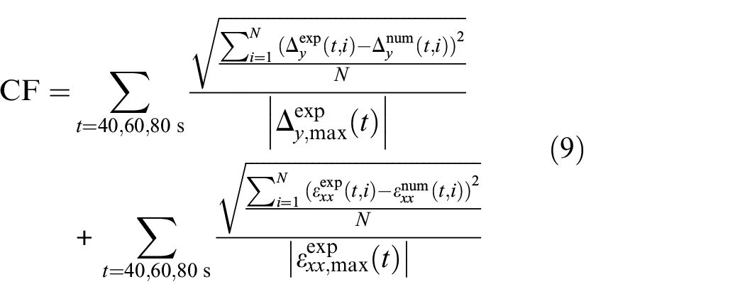
where CF is cost function, $Δ_{y}^{\exp}$ and $ε_{xx}^{\exp}$ represent the observed displacement and strain, respectively, which are obtained by considering the amount of noise, and $Δ_{y}^{num}$ and $ε_{xx}^{num}$ represent the displacement and strain extracted from the numerical model, respectively, i represents the number of each point on the grid, N is the total number of points on the grid and t represents time. Based on this function, the error value is calculated for each of the desired surfaces and finally all the values are added together to get the final value of the cost function.

Optimization process

The optimization process is an iterative process, in which the values of existing variables are changed numerous times, until the optimized values are achieved. This process consists of several steps, including interpolation of values, calculation of the cost function and finally achieving the optimal variables. In this study, a written program in Python is used to perform the optimization process. As any change in variables influence the objective results of FEM, values of displacement and strain might change as well. Therefore, by using the program written in Python, new values of variables are replaced into the Abaqus script in each loop of the optimization process. After simulating the new model, the software provides the displacement and strain values as output to Python so that the cost function can be recalculated based on the new data. The new value of the cost function is compared to the previous value, and if the results converge, the optimization process ends and the final values are presented.

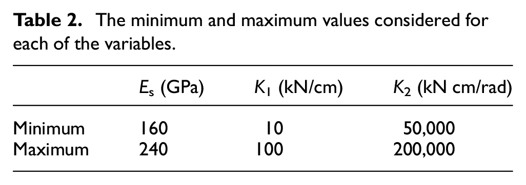
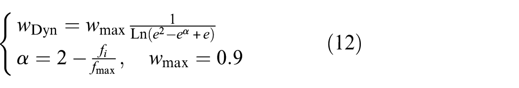
In this study, a hybrid method for optimization is used, by combining the PSO algorithm and the Powell algorithm. In the first step, PSO obtains the optimal value of each variable approximately by searching the specified ranges. In the optimization process, it is required to consider a range for each of the variables, so here a specific range is considered for each of the variables, as Dizaji et al.³⁷ The minimum and maximum values considered for each of the variables are presented in Table 2. In the second step, the values obtained in the first step are given to the Powell algorithm as an initial guess to determine the optimal values more accurately. An overview of the steps of optimization process in this research is shown in Figure 12.

Table 2.

The minimum and maximum values considered for each of the variables.

	E _s (GPa)	K ₁ (kN/cm)	K ₂ (kN cm/rad)
Minimum	160	10	50,000
Maximum	240	100	200,000

Figure 12.

An overview of the steps of optimization process in present research.

As mentioned, PSO works based on the behaviour of the birds in a swarm, which is defined as follows:

ν_{i}^{t + 1} = w ν_{i}^{t} + c_{1} r_{1} (p {best}_{i}^{t} - x_{i}^{t}) + c_{2} r_{2} (g bes t^{t} - x_{i}^{t})

(10)

x_{i}^{t + 1} = x_{i}^{t} + ν_{i}^{t + 1}

(11)

where i is the number of particles, t represents the number of the iterations, v is the velocity and x is the position of the particles. $r_{1}$ and $r_{2}$ are two random variables between 0 and 1. $c_{1}$ and $c_{2}$ are positive constants that can be adjusted and w is the weight inertia. In the PSO algorithm, the velocity and position of the particles are obtained based on the Equations (10) and (11), which determine the optimal values of the variables by moving the particles in the specified ranges. P represents the number of particles, which in this research varies between 30 and 50 based on the article by He et al.⁵³ The behaviour of the particles depends on the constants, and changing the values of these parameters can modify the results and execution time of the optimization process. $c_{1}$ and $c_{2}$ are adjustable parameters, for which three different sets are considered here. Inertia weight is one of the determining parameters in the performance of PSO algorithm. Large values of the inertia weight lead the optimization process to global minimum, while the small values are effective in achieving the local minimum. The use of dynamic inertia weight provides the opportunity to increase the ability of the PSO algorithm to quickly reach the global minimum.^53,54 Therefore, in this research, by providing a dynamic inertia weight, the computational cost is reduced and the convergence speed is increased, the dynamic inertia weight is presented as follows.

{\begin{matrix} w_{Dyn} = w_{max} \frac{1}{Ln (e^{2} - e^{α} + e)} \\ α = 2 - \frac{f_{i}}{f_{max}}, w_{max} = 0.9 \end{matrix}

(12)

where $w_{Dyn}$ is the dynamic inertia weight, $w_{max}$ is the maximum inertia weight, $f_{i}$ is the fitness of the i-th particle and $f_{max}$ is the maximum fitness of the particles. Table 3 shows the values of $c_{1}$ , $c_{2}$ , w and P for each of these groups. Final results of the optimization of finite element variables are achieved using each group of these parameters.

Table 3.

Different groups of parameters used in the PSO algorithm.

PSO parameters group	P	$c_{1}$	$c_{2}$	w
Group 1	30	2.3	1.8	$w_{max}$
Group 2	30	2.3	1.8	$w_{Dyn}$
Group 3	40	2.8	1.3	$w_{max}$
Group 4	40	2.8	1.3	$w_{Dyn}$
Group 5	50	2.05	2.05	$w_{max}$
Group 6	50	2.05	2.05	$w_{Dyn}$

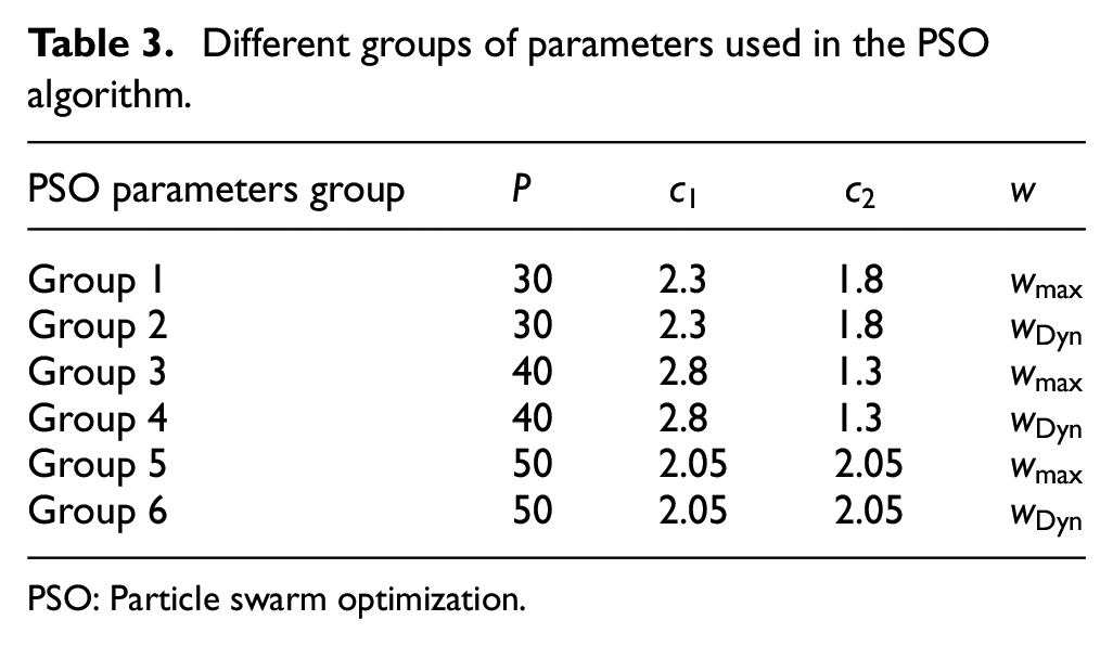
PSO: Particle swarm optimization.

Results and evaluation of the beam behaviour

In this section, at first, the results of DIC method are validated using sensors, then the performance of optimization algorithm and FEMU process are evaluated, and finally the behaviour of the beam is investigated.

Validation of the DIC method

The purpose of installing the LVDT sensor and strain gauges is to evaluate the performance of the DIC method. The amount of strain and displacement was obtained using sensors during the entire loading and unloading time; after which the performance of this method was ensured by comparing the results of the sensors with the results of the DIC method. As shown in Figure 13, the data obtained from the DIC method predict the data obtained from the LVDT sensor and strain gauges with good accuracy, so the validity of the DIC measurements is confirmed.

Figure 13.

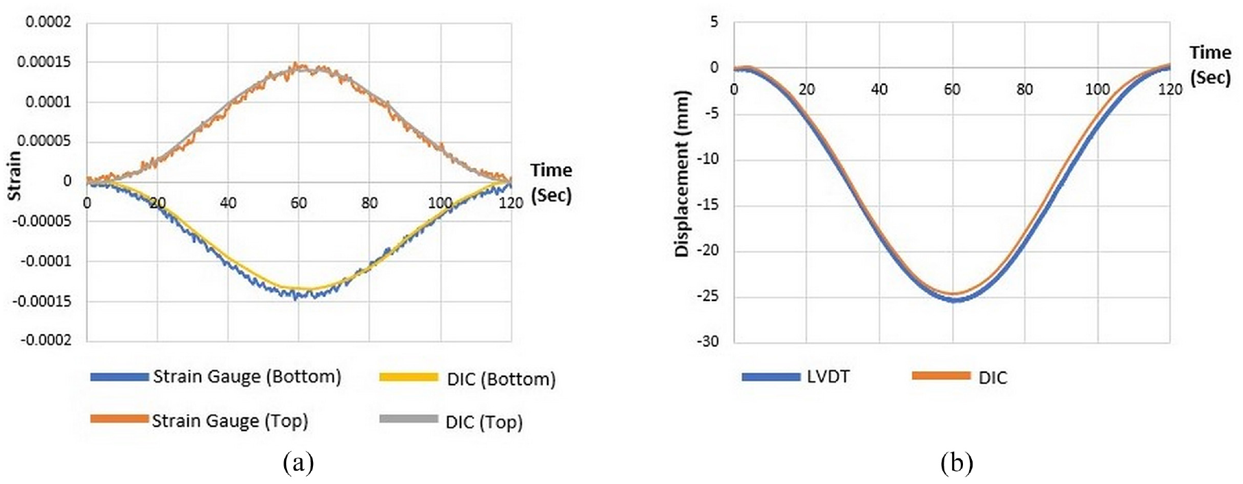
Comparison between the DIC measurements and the values obtained from the sensors: (a) Strain gauges and (b) LVDT sensor.

Evaluation of the optimization algorithm

To evaluate the performance of the optimization algorithm, various criteria are checked, which include the value of the cost function, execution time and the number of iterations. The value of the cost function for each of the groups was different at the end of the first step of optimization process, but by utilizing the Powell algorithm in the last step, all groups yielded the same value of the cost function after completing the optimization. For this reason, in this hybrid optimization method, the value of the cost function is not decisive and all groups achieve 100% search success. Therefore, to determine the performance of the presented groups, attention should be paid to the convergence speed and number of iterations. To ensure the performance of dynamic inertia weight, a comparison between the groups that have a dynamic inertia weight and the groups that have a constant inertia weight has been made as shown in Figure 14(a) to (c), in which the other parameters are the same. As can be seen, the convergence speed has increased significantly in the cases where the dynamic inertia weight has been used, which shows the appropriate performance of the presented dynamic inertia weight.

Figure 14.

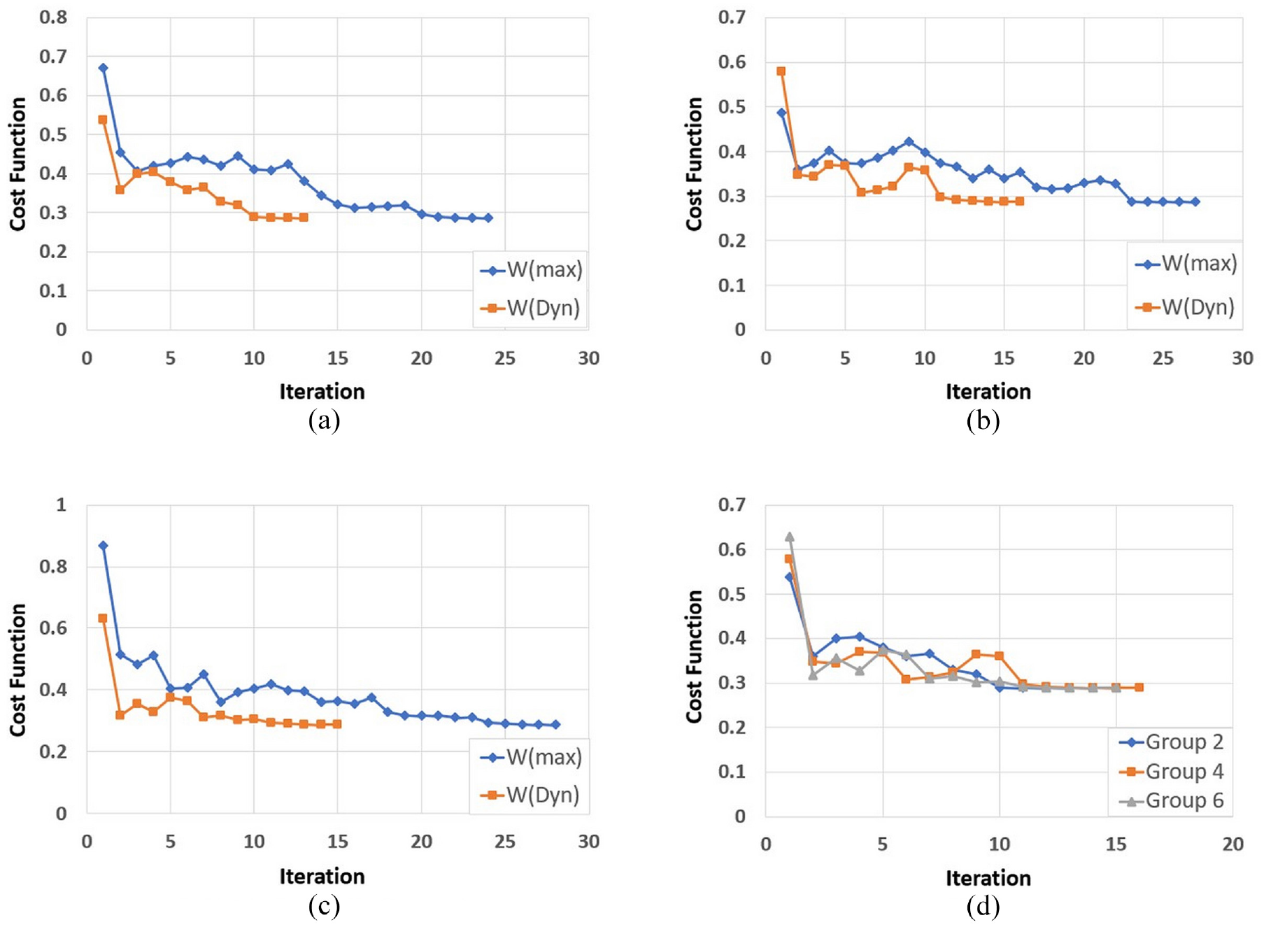
Performance comparison of the PSO algorithm: (a) Groups 1 and 2; (b) Groups 3 and 4; (c) Groups 5 and 6 and (d) Groups 2, 4 and 6.

Figure 14(d) shows the performance of groups 2, 4 and 6 in which dynamic inertia weight is used. According to the number of iterations and the convergence speed, group 2 has the best performance, and therefore the considered values for the parameters in group 2 are suitable for increasing the efficiency of the hybrid optimization method.

Performance of the FEMU process

In this section, first the importance of using the FEMU process is examined, then experimental observations are compared with numerical data at the desired surfaces, and the error of the numerical model compared with the existing structure is determined. In the following, to ensure the proper performance of the FEMU process in the entire loading and unloading time, the behaviour of the numerical model and the behaviour of specimen are compared before and after the optimization process at two specific points. Finally, the detailed and objective models are compared, and the accuracy of the models in evaluating the behaviour of the beam is determined.

To investigate the importance of using the FEMU process, a comparison is made between the initial value and the optimal value of the variables. Table 4 shows the stiffness values of the springs and the Young’s modulus before and after optimization. As it can be seen, initial values and the optimal values are different, and this difference has a great effect on the behaviour of the beam. Also, the optimal stiffness values of the springs are very different from the fully-fixed connection. Therefore, it is possible to realize the essential role of the presented FEMU process in investigating the beam behaviour.

Table 4.

The value of objective finite element model variables before and after optimization.

Variable	Initial value	Optimized value (after PSO)	Optimized value (after PPSO)
E _s (GPa)	200	232	224
K ₁ (kN/cm)	60	41	48
K ₂ (kN cm/rad)	150,000	106,400	109,200

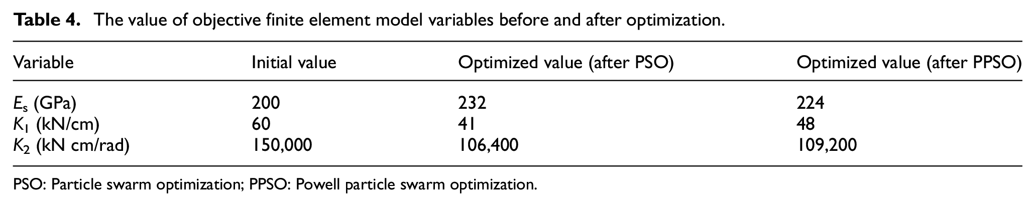
PSO: Particle swarm optimization; PPSO: Powell particle swarm optimization.

To evaluate the performance of the FEMU process, the data extracted from the optimal model are compared with the experimental observations at the desired surfaces. Figures 15 and 16 compare the displacement values obtained by the DIC method with the values obtained using the optimal FEM. In Figure 15, which shows the displacement of the beam at the free end, there are some errors between the experimental and numerical data, which can be caused by the concentrated load. Figure 17 also shows the strain of the beam at the support. It should be noted that the strain at the free end is ignored because it is very close to zero. In the support, there are some small errors in the amount of strain, which can be related to the connection, such as errors caused by welding defects.

Figure 15.

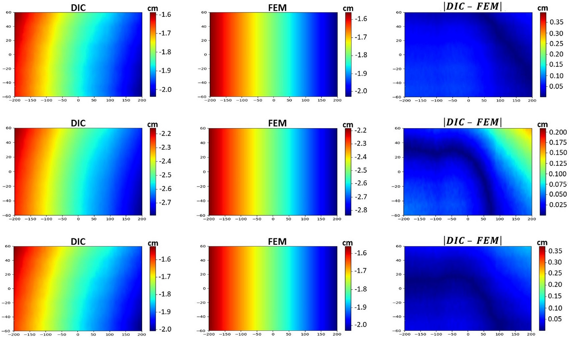
The experimental and numerical displacement fields and absolute difference at the free end (the first row for the 40 s, the second row for the 60 s and the third row for the 80 s).

Figure 16.

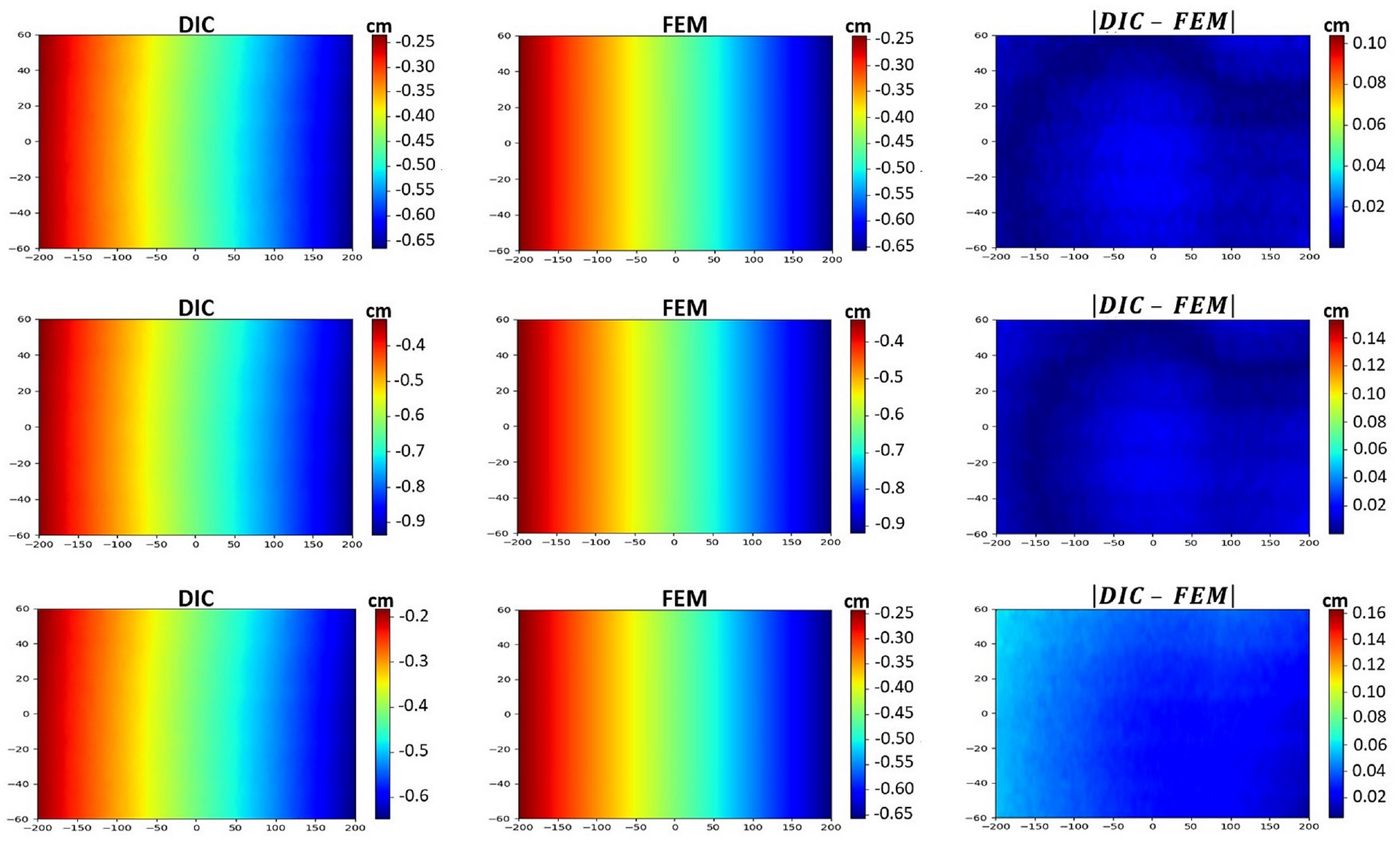
The experimental and numerical displacement fields and absolute difference at the support (the first row for the 40 s, the second row for the 60 s and the third row for the 80 s).

Figure 17.

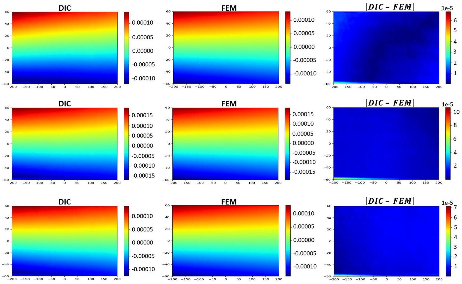
The experimental and numerical strain fields and absolute difference at the support (the first row for the 40 s, the second row for the 60 s and the third row for the 80 s).

Table 5 presents the amount of error in displacement and strain before and after optimization process. According to this table, the maximum amount of error after optimization is related to the strain of the support, which, as already mentioned, can be caused by the connection.

Table 5.

Error between experimental and numerical data before and after updating.

		Free end			Support
		Displacement			Displacement			Strain
		t = 40	t = 60	t = 80	t = 40	t = 60	t = 80	t = 40	t = 60	t = 80
NRMSE	Before updating	0.214	0.196	0.193	0.174	0.173	0.117	0.060	0.090	0.082
	After updating	0.022	0.017	0.018	0.012	0.013	0.051	0.041	0.054	0.056

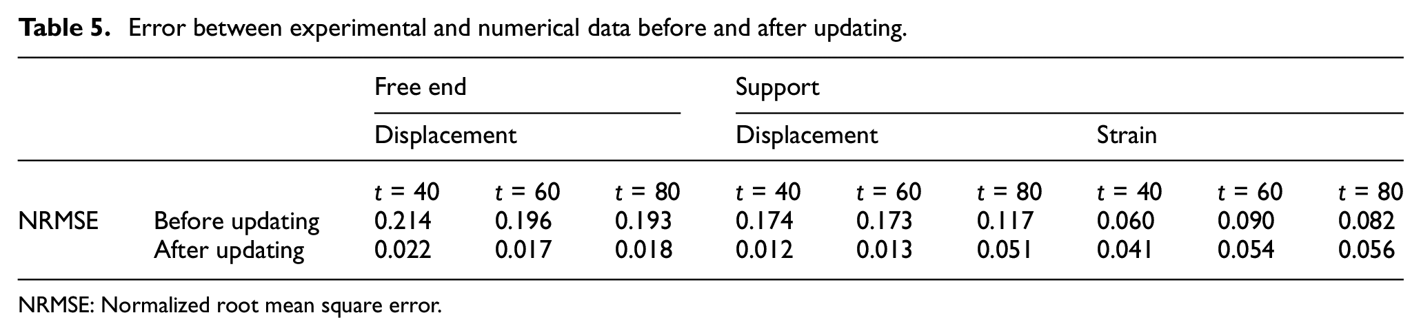
NRMSE: Normalized root mean square error.

By comparing the experimental and numerical data extracted in the 40, 60 and 80 s of the experiment, the performance of the FEMU process was investigated. To ensure the performance of FEMU process in achieving the optimal model, DIC measurements and numerical data are compared in the entire loading and unloading time at two specific points that are defined below. Figure 18 shows a comparison between DIC measurements and data obtained from the objective FEM before and after optimization at these points. The points are located on bottom of the web, the first one is at the free end of the beam where the displacement is studied, and the second one is at the beginning of the beam where the strain is investigated.

Figure 18.

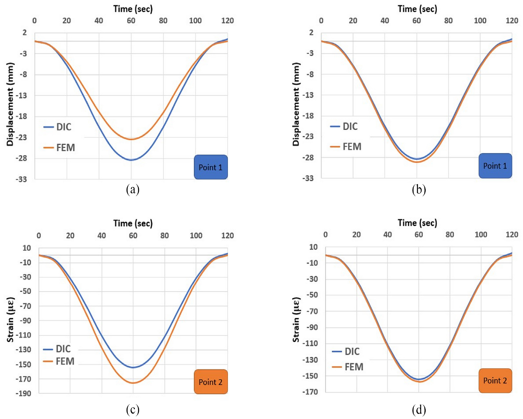
Comparison between the DIC measurements and numerical data during loading and unloading: (a and c) Before optimization and (b and d) after optimization.

According to the diagrams in Figure 18, the maximum error in the amount of displacement between the initial FEM and the DIC measurements is 5 mm, which occurs in the 60 s; however, the error is reduced to less than 0.8 mm at the end of the optimization process. Also, the maximum difference in strain value decreases from 21.5 µε to less than 3 µε. After completing the optimization process, the maximum displacement error is 2.7% of the maximum displacement obtained by the DIC, and the maximum strain error is less than 2% of the maximum strain obtained by the DIC. As can be seen in Figure 18, the behaviour of the model is well converged to the behaviour of the structure during the entire loading and unloading time, and it is expected that this model can evaluate the behaviour of the specimen under different loadings.

So far, a comparison has been made between the initial and optimal data of the objective FEM, and the results of the optimal model have been confirmed according to experimental data. For a better understanding of the effectiveness of the proposed method, the results of the detailed FEM are evaluated and compared with the optimal results. Figures 19 and 20 show the displacement and strain of the models under the maximum load applied to the beam during the test. As can be seen, the maximum displacement of the objective FEM is almost three times that of the detailed model, and the maximum strain of the detailed model is more than three times that of the objective model, which shows the inadequate accuracy of the detailed model for evaluating beam behaviour. Based on the comparison of experimental and numerical data, and the evaluation of the difference between objective and detailed FEM, it is possible to realize the appropriate performance of the presented FEMU process, which results in achieving the FEM with high accuracy.

Figure 19.

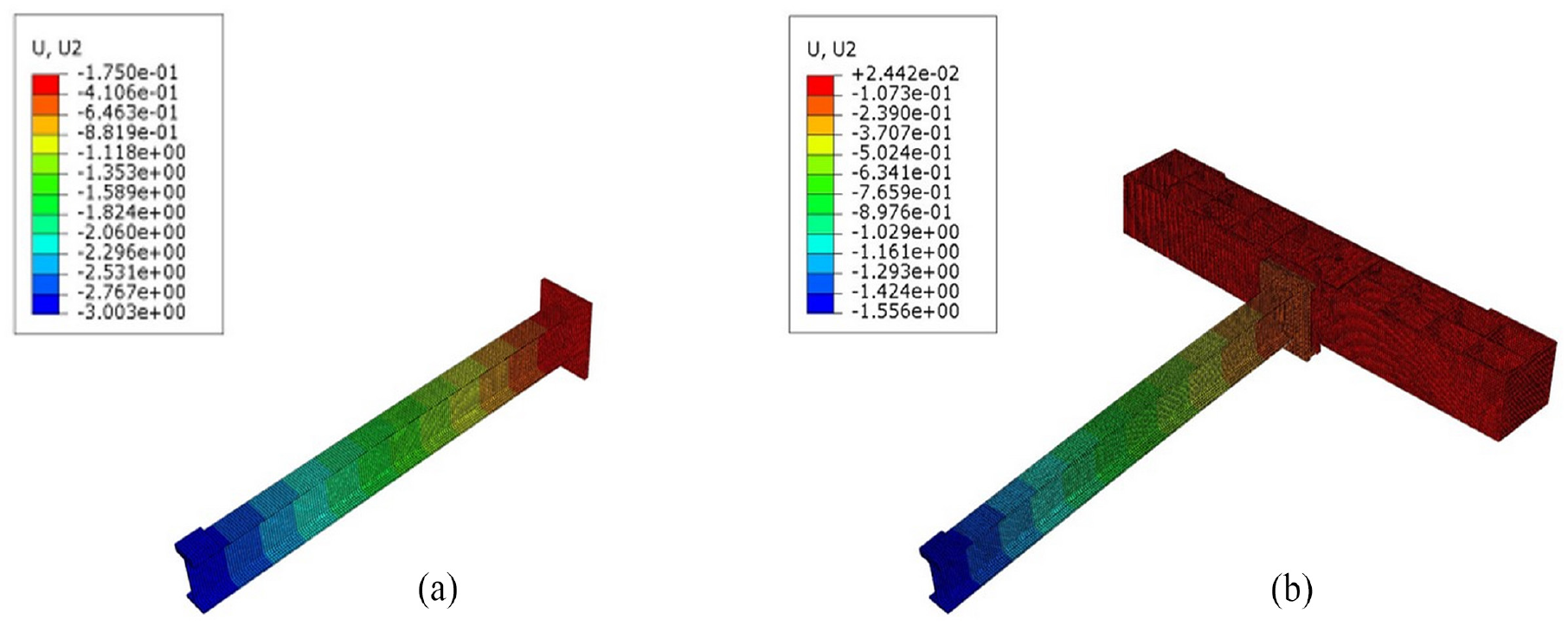
Displacement of the finite element models under the maximum load applied to the beam during the test: (a) Objective finite element model and (b) detailed finite element model.

Figure 20.

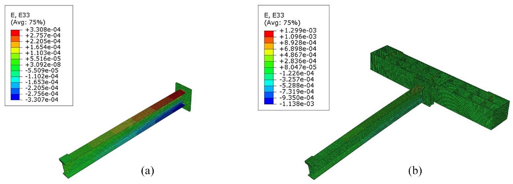
Strain of the finite element models under the maximum load applied to the beam during the test: (a) Objective finite element model and (b) detailed finite element model.

Evaluation of the beam behaviour

The vertical displacement of the support is controlled by a vertical spring and the rotation of the support is controlled by a rotational spring. The optimal stiffness values obtained for the springs adjust the vertical displacement and rotation of the connection in such a way that the FEM represents the beam behaviour well. Figure 21 shows the deformation of the beam based on the stiffness of the springs under a concentrated load of 20 kN. As can be seen in this figure, for a fixed connection, the amount of rotation and displacement of the support is zero; therefore, the stiffness of the springs is considered infinite; however, it is practically impossible to make such a connection. Figure 21(c) shows the deformation of the beam used in this study. It should be noted that the behaviour of the springs is linear and the amount of rotation and displacement of the support has a linear relationship with the applied force.

Figure 21.

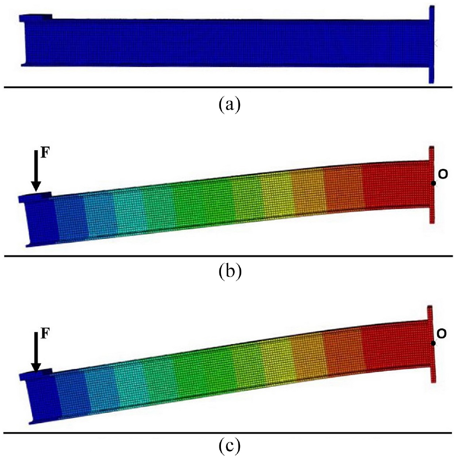
Optimal finite element model deformation: (a) Before loading; (b) the beam with fully-fixed connection and (c) the beam with partially-fixed connection.

Figure 22 evaluates the maximum displacement at the free end and maximum strain at the support of the beam under the influence of FEM variables. Changes in the Young’s modulus influence the strain of the beam and have very little effect on the amount of displacement. Furthermore, changes in the amount of stiffness of the springs have no effect in the amount of strain, that is why its diagrams have been omitted.

Figure 22.

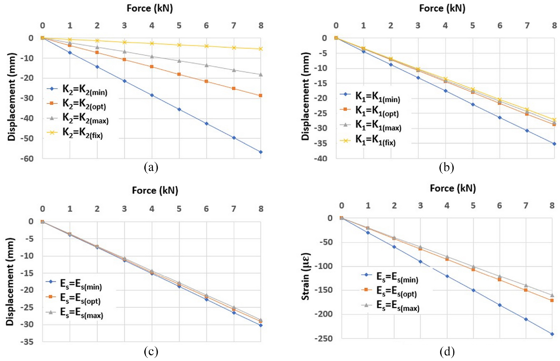
The dependence of beam behaviour based on changes in the values of variables. (a) E_s = E_s(opt), K₁ = K_1(opt),(b) E_s = E_s(opt), K₂ = K_2(opt), (c) K₁ = K_1(opt), K₂ = K_2(opt) and (d) K₁ = K_1(opt), K₂ = K_2(opt).

According to Figure 22, displacement of the beam is highly dependent on the stiffness of the springs, while the dependence on the Young’s modulus is much lower. In Figure 22(a), due to the wide range of changes in the displacement of the cantilever beam, it is necessary to investigate its displacement with the optimal FEM, because it can cause damage to structural and non-structural components.

Figure 23 shows the ratio of the maximum displacement of the beam as a function of stiffness of the springs to the maximum displacement of the fully-fixed beam. Rotational spring stiffness has more influence on the displacement of the beam than the vertical spring stiffness. The rate of changes in the amount of displacement based on the springs stiffness is nonlinear, so that in low stiffness values the rate of changes is high, but in high stiffness values the rate of changes is lower. It should be noted that the effect of changes in spring stiffness is independent of each other.

Figure 23.

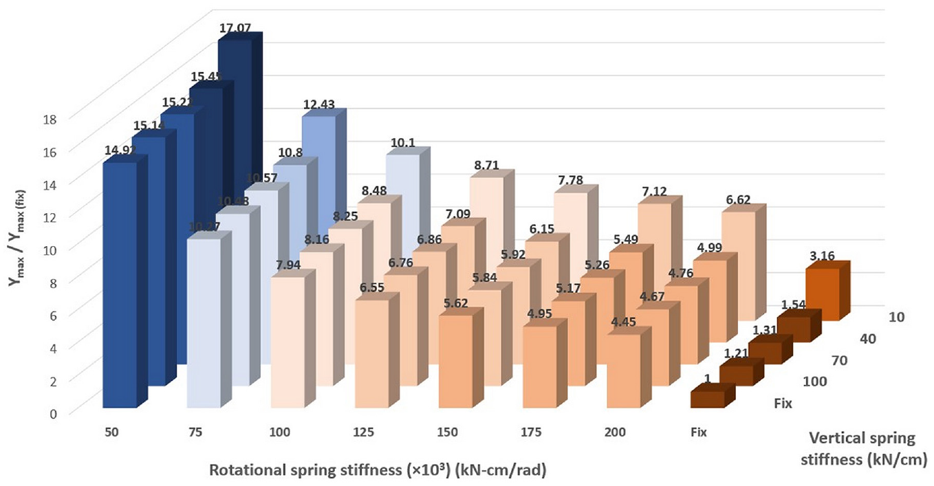
The ratio of the maximum displacement of the beam as a function of stiffness of the springs to the maximum displacement of the fully-fixed beam.

Summary and conclusions

Behaviour evaluation of structures based on existing conditions is of great importance. The FEMU method is one of the reliable methods to study the behaviour of structures based on existing conditions. This method is based on data acquisition from the structure and minimizing the error between the FEM and the existing structure.

In this paper, using a FEMU method based on DIC, which is a full field measurement technique, and PPSO, which is a hybrid optimization method, the behaviour of a cantilever beam was investigated. The presented FEMU process studies the behaviour of beams under the influence of different conditions and based on the connection behaviour, which is utilized for cantilever beams with different types of connections. Here, the beam has a partially-fixed connection, which significantly influences the behaviour of the beam. FEM variables include vertical spring stiffness and rotational spring stiffness in the support and Young’s modulus. The optimal values of the FEM variables are obtained using DIC measurement. The behaviour of the beam is investigated using optimal FEM. The data extracted by DIC method are validated using sensors installed on the specimen.

The PPSO algorithm provides acceptable results, and the optimal values of the FEM variables have an acceptable error compared to the experimental data. The presented dynamic inertia weight accelerates the optimization process to achieve the optimal result and shows appropriate performance compared to the constant inertia weight.

Due to the difference between the initial and optimal values of the variables and its great influence on the behaviour of the model, the importance of using the FEMU process is confirmed. To evaluate the performance of the FEMU process, after optimizing the model using the FEMU process, the error between numerical data and experimental observations was calculated based on NRMSE, and it was found that the maximum error value after optimization is 0.056, which is acceptable. By comparing the error value before and after optimization, the appropriate performance of FEMU process is confirmed. Finally, a comparison was made between the objective FEM and the detailed model, and it was found that the objective model had much less error than the real structure.

The FEMU process provides the possibility of obtaining a FEM with high accuracy, which has the ability to evaluate the behaviour of the specimen. The behaviour of the beam is very different from the fully-fixed beam and from the initial model. The maximum displacement of the beam is much higher than that of a fully-fixed beam, which indicates the low stiffness of the connection. The effect of changes in the FEM variables on the behaviour of the beam is investigated. The rotational spring simulated on the support has the greatest effect on the vertical displacement of the beam, so that low values of spring stiffness caused large displacements at free end of the beam. The Young’s modulus has very little effect on the amount of displacement of the beam, and its main effect is on the strain.

The FEMU approach can be extended to other structural components with various connection arrangements. In the FEMU method, using different data acquisition methods, selecting different variables to simulate the FEM and using different optimization methods can improve the performance of the updating process.

Footnotes

Acknowledgements

The authors wish to thank all people who helped in conducting this research, especially Mohsen Zanganeh, the assistant of the Structural Dynamics Strong Floor laboratory at the Sharif University of Technology (SUT), and Salar Zeinali for their kind help.

Declaration of conflicting interests

The author(s) declared no potential conflicts of interest with respect to the research, authorship, and/or publication of this article.

Funding

The author(s) received no financial support for the research, authorship, and/or publication of this article.

ORCID iDs

Alireza Khaloo

Amirhossein Amirahmadi

References

Oguibe

Webb

. Large deflection analysis of multilayer cantilever beams subjected to impulse loading. Comput Struct 2000; 78: 537–547.

Yang

H-S

Chung

H-J

Park

Y-J

. Stress analysis of a cantilevered fixed partial denture with normal and reduced bone support. J Prosthet Dent 1996; 76: 424–430.

Sim

H-B

Uang

C-M

. Repair of damaged welded connections in cantilevered steel sign structures. Eng Struct 2014; 67: 19–28.

Alver

Selman

Akgun

. The effect of short cantilever beam formation on the structural behavior of precast post-tensioned connections. Constr Build Mater 2012; 35: 232–239.

Sajjanapu

Ward

. Vibration of a semi-rigid cantilever in a uniform flow. J Fluids Struct 2021; 102: 103229.

Kartal

Basaga

Bayraktar

, et al. Effects of semi-rigid connection on structural responses. Electron J Struct Eng 2010; 10: 22–35.

Markazi

Beale

Godley

MHR

. Experimental analysis of semi-rigid boltless connectors. Thin-Walled Struct 1997; 28: 57–87.

Karbhari

Ansari

(eds). Structural health monitoring of civil infrastructure systems. Elsevier: US 2009.

Mishra

. Machine learning techniques for structural health monitoring of heritage buildings: a state-of-the-art review and case studies. J Cult Herit 2021; 47: 227–245.

10.

Sarmadi

Yuen

K-V

. Structural health monitoring by a novel probabilistic machine learning method based on extreme value theory and mixture quantile modeling. Mech Syst Signal Process 2022; 173: 109049.

11.

Zhang

Mousavi

Masri

, et al. Vibration feature extraction using signal processing techniques for structural health monitoring: a review. Mech Syst Signal Process 2022; 177: 109175.

12.

Ngeljaratan

Moustafa

. Structural health monitoring and seismic response assessment of bridge structures using target-tracking digital image correlation. Eng Struct 2020; 213: 110551.

13.

Khalilzadehtabrizi

Seifiasl

Hoseinzadeh Asl

. Measurement of deformation patterns in steel plate shear walls subjected to cyclic loading based on multi-target digital image correlation (MT-DIC). Structures 2021; 33: 2611–2627.

14.

Seventekidis

Giagopoulos

. A combined finite element and hierarchical deep learning approach for structural health monitoring: test on a pin-joint composite truss structure. Mech Syst Signal Process 2021; 157: 107735.

15.

Wani

Khan

Vemuri

. 2D nonlinear finite element analysis of reinforced concrete beams using total strain crack model. Mater Today Proc 2022; 64: 1305–1313.

16.

Xiong

, et al. A comprehensive study on CFRP rapid portable bridge: design, experimental investigation and finite element analysis. Compos Struct 2022; 289: 115439.

17.

Lin

Y-L

, et al. Time history analysis-based nonlinear finite element model updating for a long-span cable-stayed bridge. Struct Health Monit 2020; 147592172096386.

18.

Zhang

Sun

. Structural damage identification via physics-guided machine learning: a methodology integrating pattern recognition with finite element model updating. Struct Health Monit 2021; 20: 1675–1688.

19.

Avci

Alkhamis

Abdeljaber

, et al. Operational modal analysis and finite element model updating of a 230 m tall tower. Structures 2022; 37: 154–167.

20.

Xia

P-Q

Brownjohn

JMW

. Residual stiffness assessment of structurally failed reinforced concrete structure by dynamic testing and finite element model updating. Exp Mech 2003; 43: 372–378.

21.

Naranjo-Pérez

Infantes

Fernando Jiménez-Alonso

, et al. A collaborative machine learning-optimization algorithm to improve the finite element model updating of civil engineering structures. Eng Struct 2020; 225: 111327.

22.

Eiras

Payan

Rakotonarivo

, et al. Experimental modal analysis and finite element model updating for structural health monitoring of reinforced concrete radioactive waste packages. Constr Build Mater 2018; 180: 531–543.

23.

Razavi

Hadidi

. Structural damage identification through sensitivity-based finite element model updating and wavelet packet transform component energy. Structures 2021; 33: 4857–4870.

24.

Modak

Kundra

Nakra

. Comparative study of model updating methods using simulated experimental data. Comput Struct 2002; 80: 437–447.

25.

Kumar Bagha

Gupta

Panwar

. Finite element model updating of a composite material beam using direct updating method. Mater Today Proc 2020; 27: 1947–1950.

26.

Verma

Kango

Bagha

, et al. Finite element model updating of smart structures with direct updating algorithm. Phys Scr 2022; 97: 055702.

27.

Lei

Wang

Shen

. Update the finite element model of Canton Tower based on direct matrix updating with incomplete modal data. Smart Struct Syst 2012; 10: 471–483.

28.

Mottershead

Link

Friswell

. The sensitivity method in finite element model updating: a tutorial. Mech Syst Signal Process 2011; 25: 2275–2296.

29.

Chen

Huang

. Updating finite element model using dynamic perturbation method and regularization algorithm. Smart Struct Syst 2012; 10: 427–442.

30.

Chen

H-P

Y-Q

. Structural health monitoring of large civil engineering structures. Chichester, UK: John Wiley & Sons, Ltd, 2018. Epub ahead of print 12 March 2018. DOI: 10.1002/9781119166641.

31.

Arora

. Comparative study of finite element model updating methods. J Vibr Control 2011; 17: 2023–2039.

32.

Biscaia

Canejo

Zhang

, et al. Using digital image correlation to evaluate the bond between carbon fibre-reinforced polymers and timber. Struct Health Monit 2022; 21: 534–557.

33.

Lima

RAA

Perrone

Carboni

, et al. Experimental analysis of mode I crack propagation in adhesively bonded joints by optical backscatter reflectometry and comparison with digital image correlation. Theor Appl Fract Mech 2021; 116: 103117.

34.

Chen

Ning

. Identification of fracture damage characteristics in ultra-high performance cement-based composite using digital image correlation and acoustic emission techniques. Compos Struct 2022; 291: 115612.

35.

Dizaji

Harris

Alipour

. Integrating visual sensing and structural identification using 3D-digital image correlation and topology optimization to detect and reconstruct the 3D geometry of structural damage. Struct Health Monit 2022; 21: 2804–2833.

36.

Mayo-Corrochano

Sánchez-Aparicio

Aira

J-R

, et al. Assessment of the elastic properties of high-fired gypsum using the digital image correlation method. Constr Build Mater 2022; 317: 125945.

37.

Shafiei Dizaji

Alipour

Harris

. Leveraging full-field measurement from 3D digital image correlation for structural identification. Exp Mech 2018; 58: 1049–1066.

38.

Pan

Qian

Xie

, et al. Two-dimensional digital image correlation for in-plane displacement and strain measurement: a review. Meas Sci Technol 2009; 20: 062001.

39.

Korswagen

Longo

Rots

. High-resolution monitoring of the initial development of cracks in experimental masonry shear walls and their reproduction in finite element models. Eng Struct 2020; 211: 110365.

40.

Hofmeister

Bruns

Rolfes

. Finite element model updating using deterministic optimisation: a global pattern search approach. Eng Struct 2019; 195: 373–381.

41.

Keivanian

Chiong

. A novel hybrid fuzzy–metaheuristic approach for multimodal single and multi-objective optimization problems. Expert Syst Appl 2022; 195: 116199.

42.

Rastogi

Srivastava

Tarun , et al. A hybrid optimization approach using PSO and ant colony in wireless sensor network. Mater Today Proc. Epub ahead of print 6 March 2021. DOI: 10.1016/j.matpr.2021.01.874.

43.

Jiang

Zhao

. Structural deformation prediction model based on extreme learning machine algorithm and particle swarm optimization. Struct Health Monit 2022; 21: 2786–2803.

44.

Kim

Chang Jung

, et al. Optimal sensor placement to detect ruptures in pipeline systems subject to uncertainty using an Adam-mutated genetic algorithm. Struct Health Monit 2022; 21: 2354–2369.

45.

Guo

Yuan

Dang

, et al. Cable force optimization of a curved cable-stayed bridge with combined simulated annealing method and cubic B-Spline interpolation curves. Eng Struct 2019; 201: 109813.

46.

Dillen

Lombaert

Schevenels

. A hybrid gradient-based/metaheuristic method for Eurocode-compliant size, shape and topology optimization of steel structures. Eng Struct 2021; 239: 112137.

47.

Liu

Han

, et al. A particle swarm optimization–support vector machine hybrid system with acoustic emission on damage degree judgment of carbon fiber reinforced polymer cables. Struct Health Monit 2021; 20: 1551–1562.

48.

Engelbrecht

. Computational intelligence an introduction. John Wiley & Sons Ltd: UK, 2007.

49.

Fürer

Floudas

Christodoulos A.

Pardalos

Panos M.

Parallel computing: complexity classes. In: Floudas

Christodoulos A.

Pardalos

Panos M.

(eds) Encyclopedia of Optimization. Boston, MA: Springer US, 2008, pp. 2900–2903.

50.

European standards. Hot rolled I and H sections (IPE series); dimensions, mass and static parameters. DIN 1025-5, 1994.

51.

https://www.gom.com/

52.

Liu

Quek

. Finite element method. Elsevier: USA, 2003.

53.

Zhang

. The parameters selection of PSO algorithm influencing on performance of fault diagnosis. MATEC Web Conf 2016; 63: 02019.

54.

Jiao

Lian

. A dynamic inertia weight particle swarm optimization algorithm. Chaos Soliton Fract 2008; 37: 698–705.

Performance assessment of steel cantilever beams based on connection behaviour using DIC technique and improved hybrid PSO algorithm

Abstract

Keywords

Introduction

Experimental study

Test setup

End connection of beam

Loading

Digital image correlation

Numerical study

Finite element model

Theory of the objective FEM

Cost function

Optimization process

Results and evaluation of the beam behaviour

Validation of the DIC method

Evaluation of the optimization algorithm

Performance of the FEMU process

Evaluation of the beam behaviour

Summary and conclusions

Footnotes

Acknowledgements

Declaration of conflicting interests

Funding

ORCID iDs

References