
Abstract
Civil and maritime engineering systems must be efficiently managed to control the failure risk at an acceptable level as their performance is gradually degraded throughout the operational life, caused by fatigue and corrosion. Structural health monitoring develops a timely capability to assess the structural condition and performance metrics. However, using actual long-term monitoring data to guide the life-cycle management under stochastic environments has not been sufficiently studied. To realize an optimal maintenance strategy within the service life, an integrated monitoring-based optimal management framework is developed on the basis of the partially observable Markov decision processes (POMDPs) and Bayesian forecasting. In the proposed framework, the stochastic fatigue processes are quantified by the state transition matrix. The Bayesian dynamic linear model is embedded in POMDPs as a continuous observation part to forecast the cycling impacts and estimate the deterioration rate using long-term dynamic strain responses. In addition, making use of the special features of the problem considered in this paper, an adaptive discretization strategy is proposed to alleviate the complexity of large discrete observed spaces in the POMDP. The applicability and feasibility of the framework are evaluated by intelligent maintenance of fatigue-sensitive components with real-world monitoring data. After solving the POMDP by an efficient offline solver, the results obtained in this paper demonstrate that structural interventions are uneconomical to extend the life when a welded detail is approaching its end of life due to the normal service. Furthermore, if multiple interventions are available, the framework can find optimal maintenance actions based on the trade-off between long-term utility and the corresponding cost. This framework as the prototype could also be adjusted to aid life-cycle intelligent maintenance of other types of components under different deterioration scenarios.
Keywords
Introduction
Within the service life of an engineered structure, it could be subjected to different deterioration scenarios (e.g., corrosion, fatigue), which could affect the serviceability and functionality of the structure. For instance, Wardhana and Hadipriono 1 summarized failures of bridge structures in the United States between 1989 and 2000 and found 11 bridges failed due to fatigue. In addition, fatigue of ship critical details has always been the main concern for ship operation and is one of the deterioration mechanisms that can affect structural performance. Under these circumstances, decision-makers are faced with fatigue failure risk and must distribute limited budgets so that the component can be operated safely during the life cycle. These facts highlight the importance of an effective decision-making system for the vulnerable infrastructure in the years to come, and underscore the imperative need for developing versatile and intelligent decision-support frameworks that can serve multi-purpose real-time and life-cycle objectives. Motivated by the evolution of cutting-edge monitoring technologies, reliable transducers, and effective information processing algorithms, structural health monitoring (SHM) systems develop a real-time data-driven performance-based assessment ability which is the precondition of rational maintenance. Accordingly, developing decision-support systems for infrastructure management based on real-world monitoring data becomes possible and necessary.
In this paper, fatigue assessment based on long-term monitoring data is conducted. Through reviews of the successful cases in SHM, the fatigue of the steel components is usually assessed by the rain-flow algorithm and linear cumulative damage theory. Ni et al. 2 proposed a fatigue reliability model which integrates the distribution of the T-joint stress range with Miner’s damage cumulative rule to estimate the fatigue life with long-term monitoring data. At the structural level, Ye et al. 3 proposed a monitoring-based method for the fatigue assessment of Tsing Ma bridges by using the continuously measured dynamic strain responses. Furthermore, Farreras-Alcover et al. 4 incorporated monitoring data with the S–N model to estimate the residual service life of welded joints in the Great Belt Bridge. Herein, to enhance the compatibility associated with different types of data, the Markov chain model is proposed to assess the fatigue process. This model can express a non-stationary state deterioration based on inspection data, dynamic fatigue degradation rested on monitoring data, and is rooted in the stochastic process.
SHM is recognized as a feasible field facilitating to secure the operational safety of structures and prognosis of the damage in time to prevent additional maintenance costs or catastrophic failure. 5 This is attributed to the capability of the SHM system in monitoring the impacts actually acting on the vulnerable components. SHM provides an insight into the structures undergoing gradual changes in condition. For fatigue component management, one of the underlying requirements is to rationally forecast cycling impacts based on the long-term strain responses. However, it poses a challenge in the practical application of prediction when facing the uncertainty and non-stationary features inherent in the monitoring data. To solve this aspect, different forecasting algorithms have been widely studied and attempted, for instance, the statistical models, 6 time series models, 7 gray system theory, 8 and singular spectrum model. 9 More recently, the Bayesian forecasting model has been applied in real-world data prediction due to its merits. Bayesian dynamic linear model (BDLM) can automatically accommodate non-stationary time series data through time-varying model parameters, 10 which increases the robustness to tackle data missing. In addition, BDLM can adjust the model parameters through newly obtained observations and provide ahead forecasts without reconstructing models, and it can consider the uncertainty in monitoring data and quantifying the probabilistic distribution in forecasting. 11 These advantages motivate the BDLM favorably for forecasting the performance of an in-service structure based on long-term monitoring data. For instance, Ni et al. 12 employed this model in expansion joints assessment and damage alarm on the basis of the long-term displacement and temperature data. Wang and Ni 13 also used BDLMs to predict the structural strain response. Although establishing a BDLM using SHM data is achievable, life-cycle maintenance of fatigue-sensitive components incorporating the long-term SHM data and predicted dynamic strain responses resulting from BDLM has not been well investigated. In this paper, BDLM is constructed to estimate the daily cumulative damage based on real-world dynamic strains and delineate the fatigue development by using different hidden blocks, such as overall trend, seasonal, and auto-regressive (AR). Moreover, predictions made available by BDLM are essential for the decision-maker to make more informed and rational maintenance actions on a time scale.
Another key step in infrastructure management is how to exploit prior information and long-term monitoring data to guide optimal maintenance. Some difficulties are associated with (i) incomplete information about the structural condition, (ii) state stochastic degradation and random outcome of maintenance, and (iii) long-term objectives. The majority of the models14–17 in infrastructure management cannot simultaneously account for the above three paramount factors. The frameworks that satisfy three requirements18–20 are solely feasible in simulation models without being compatible with the actual data (e.g., inspection, monitoring data). More realistic decision models are needed to develop in infrastructure management facing real data and uncertainty. These sequential decision-making models can be classified as genetic algorithm (GA), decision tree, and dynamic programming. The GA in optimal maintenance has been systematically studied.21–23 Through setting genetic operators and mutation, the GA can search for the optimal strategy under multi-objectives. However, heavier computation leads to the low convergence speed of GA in complex decision problems. The decision tree 24 reduces the computation cost by setting a series of criteria to determine maintenance actions. This method is realized in high efficiency but may result in a feasible scheme rather than the optimal solution. In recent studies, dynamic programming methods in the robotic control field have been applied in infrastructure management. An approach referred to as the partially observable Markov decision processes (POMDPs) in dynamic programming provides a well-suited framework for maintenance in structural stochastic degradation under imperfect observation. Due to the sound life-cycle optimality guarantees and good convergence property, 25 POMDPs are employed in highway pavement maintenance, 19 deck structure, 26 and bridge component management. 27 It is also employed to consider the value of information for the SHM system.28–30 However, the aforementioned studies are restricted to numerical studies and existing research lacks sufficient attention to how to verify and update some assumptions, such as discrete observation value and stationary state transition matrix in traditional POMDPs, 31 by incorporating the long-term health monitoring data. To accommodate the dynamic deterioration process and actual monitoring data, the solver for non-stationary 32 and continuous observation POMDP 33 should be utilized. However, most online solvers use limiting steps lookahead exploration methods or artificially discretize the observation space to reduce the computation to a tractable level. 34 This simplification may induce the policy to fall into the sub-optimal solution. 35 Lim et al. 36 pointed out that there are no theoretically guaranteed online solvers that can find optimal solutions with the limit of finite computational resources. Until now, solving POMDPs with continuous observation spaces in an uncertain environment remains challenging. 37 In summary, to address the optimal decision-making problem for welded details, the model should address two issues: (1) establish a quantified model for structural informatics, probabilistic performance prediction, risk management, and control by incorporating real-world long-term health monitoring data. (2) Use a highly efficient algorithm to compute optimal or near-optimal solutions.
In this paper, an intelligent decision-support framework is proposed for welded details management based on long-term real-world monitoring data and POMDPs. The primary functions of the framework include a database from SHM, structural condition assessment, degradation prediction, life-cycle cost, and decision-making. The fatigue deterioration model is developed by using long-term health monitoring data and quantified by the Markov chain. The dynamic strain response of welded details is embedded into the observation part of POMDPs which successively update the prior information on structural conditions using the monitoring data to guide the decision-making. Furthermore, this study develops an efficient discretization strategy on the basis of the features of the state transition matrix and reward matrix in infrastructure management to tackle continuous observation spaces. The remainder of the paper is organized as follows: Methodology presents the Markov chain-based approach for fatigue assessment, the BDLM, and the continuous observation POMDPs. Subsequently, Illustrative example describes the application of the proposed model in life-cycle optimal maintenance of welded details under partially observable stochastic environments. The maintenance results are discussed in Results and discussions, before drawing conclusions. In summary, this study aims to: (i) use the Markov chain to describe the probabilistic fatigue damage process; (ii) establish the BDLMs with different regressive blocks incorporating the long-term monitoring data; (iii) design an adaptive discretization strategy for POMDPs with continuous observation spaces based on the features of infrastructure management; and (iv) establish an optimal maintenance policy-making framework using long-term monitoring data. It can (1) avoid theoretical inconsistencies of existing studies, (2) be compatible with various statistical models and advanced sequential decision-making algorithms, and (3) give optimal maintenance policy to the decision-makers.
Methodology
In this section, the developed computational flowchart by incorporating the algorithms in the framework is illustrated in Figure 1, which includes the Markov chain in fatigue assessment, and BDLMs in fatigue deterioration prediction. The continuous POMDPs are explained in how it formulates infrastructure management. The flow chart is shown in Figure 1.
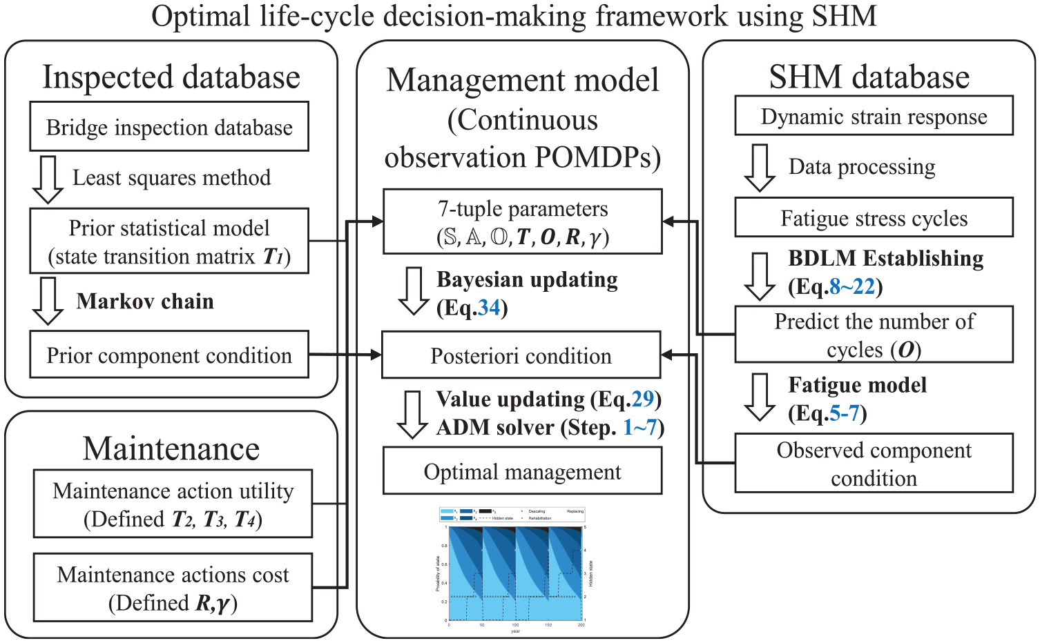
Optimal life-cycle management framework to consider stochastic deterioration components based on long-term monitoring data. The bold words denote the algorithms introduced in this paper.
Markov-chain-based fatigue assessment
This part introduces the assessment of the cumulative fatigue damage via the Markov chain. The model uses discrete states and stochastic state-transition probabilities to describe the fatigue process, which is identical to the concept of state transition in POMDP. Generally, there exist two conventional methods for fatigue assessment. The crack growth model describes the possible crack propagation during the stress cycles. S–N curve model focuses on failure probability after the structure suffers stress cycles. The Markov chain model retains the properties of the above two models, which can define different physical states to express the crack expansion or the failure probability.
Fatigue model
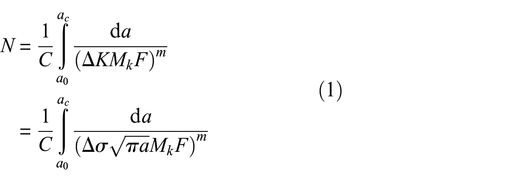
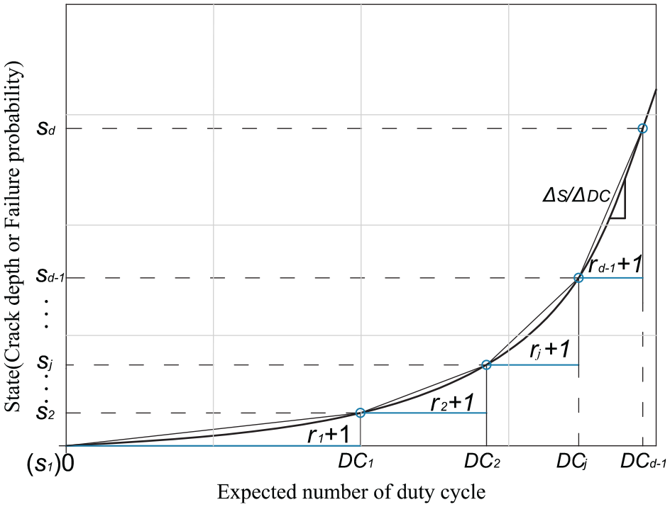
Fatigue describes the blunting and re-sharpening advancing progress of a crack front with increasing and decreasing stresses respectively during load cycles. One characteristic of fatigue is the uncertainty of crack development as depicted in Figure 2 which uses different colors to distinguish confidence intervals. The expected crack growth function (black line in Figure 2) in the welded details thickness direction is given as 38 :
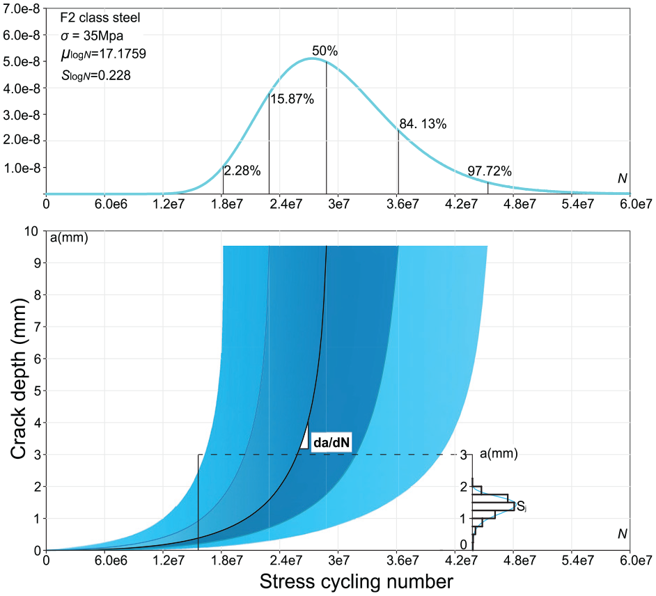
Crack development curve. The crack in fatigue presents slow growth in early stage and rapid propagation close to failure.
Equation (1) indicates the expected cycling number N of the crack growth from the lower limit
To simplify Equation (1), the S–N curve model is introduced to present a bilinear relation between the stress amplitude

where m is the slope of a linear function, and
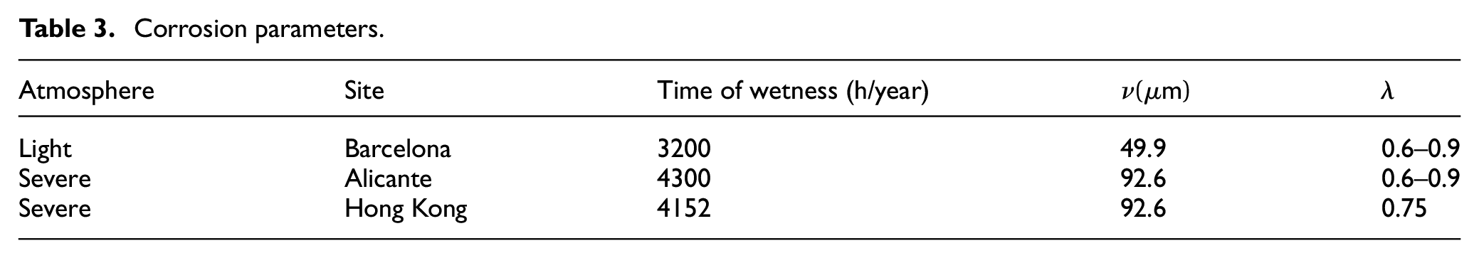
For fatigue analysis, corrosion is an essential parameter since the fatigue life of welded details in the marine environment is significantly lower than in dry air. The corrosion of the welded details can be approximately divided into three phases. 42 In the first phase, the corrosion happens at the welded area due to the stress concentration which could trigger coating disabling protection. In phase 2, moderate corrosion weakens the cross-section and induces the principal stress increase. In phase 3, the welded toe loses mass which induces severe damage to the details. To quantify the corrosion in the component life-cycle, an approximate estimation method is proposed 43 :

where M refers to the mass loss. In welded details, as the size of the thickness direction is much less than the other two dimensions, M is equivalent to the thickness reduction.
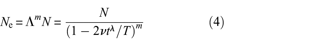
where
Markov Chain model
The Markov chain model is employed because it not only represents the stochastic degradation process but simplifies complex mathematical operations, such as integration in Equation (1). The Markov chain is related to the state transition. It uses the probability transition matrix to describe a component state
The following step is to build the numerical expression between failure probability and DC in the Markov chain model. Different from the S–N model, the fatigue process in the Markov chain is expressed by state vector transform in the matrix, where the state is defined as reliability. The unit-jump matrix is assumed to denote the state transition in a DC based on the statistical inspection results, 48 defined as 49 :
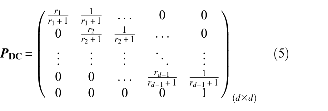
The unit-jump assumes that the current state can only degenerate to an adjacent higher state in a DC. In Equation (5), the argument
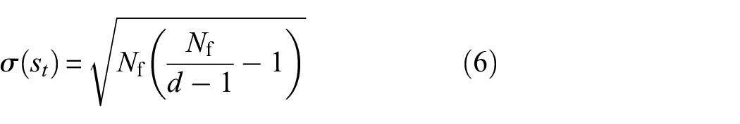
The parameters’ standard deviation
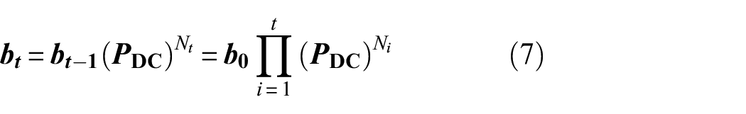
It should be noted that the latter part of Equation (7) assumes
- Initial damage can be incorporated into the model via setting the initial condition vector
- The evolution of damage can be traced at any moment.
- The accelerated fatigue damage process is approximated by different STRs
- Uncertainty is quantified as
The Markov chain model plays as an important role in connecting different algorithms in the integrated management framework. Through Equation (7), the monitoring data is transferred into the probabilistic distribution of the belief state
The fatigue process is described in the Markov chain model.
Bayesian dynamic linear models
An appropriate maintenance strategy should consider the current component condition and the deterioration rate in the future. Thus, a prediction method named BDLM is employed in this study. The fundamental background theories of AR and Kalman filtering (KF) which are embedded within the BDLM are not discussed for brevity. The BDLM has shown promising merits in the field of SHM. The flexibility in BDLM allows it to incorporate various regressive blocks to reflect the characters of data. In addition, it also considers the relationship between different blocks through covariance. Since KF is rooted in the updating process, BDLM has robustness to deal the cases with distortion or incomplete data.
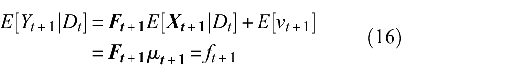
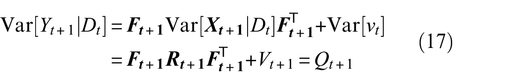
BDLM contains two parts, the dynamic linear model (DLM) and the Bayesian method to update the model parameters. For DLM, the observation equation and system evolution equation are implemented to describe the dynamic changing of monitoring data. Define Y as the dynamic response of structure based on SHM sampling.

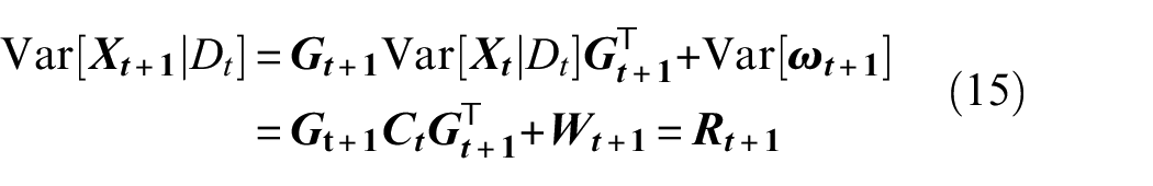
Since the

where
The recursive process in DLM indicates the initial variable
Block component
Theoretically, BDLM can combine any mathematical functions which are utilized to describe a changing rule, such as linear growth, accelerated increasing, periodic fluctuation in Fourier form, periodic oscillation in Kernel regression form, and AR. For stress cycling prediction, three-block components are employed: (a) a trend component, (b) a seasonal component, and (c) an AR component.
The trend is the most fundamental component in the forecast model which describes a steady variation in time series. This component can be expressed using polynomial functions. Normally, second-order polynomials are recommended to avoid the overfitting problem when using higher-order polynomials, the matrix pattern is given as 11 :
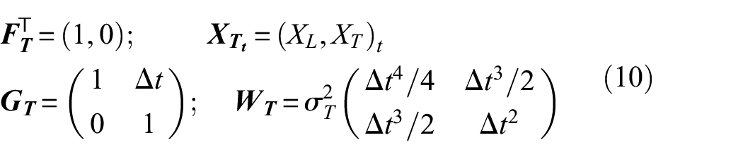
where subscript T denotes that the above parameters are related to the trend component. Additionally, any arguments evolving with the time series are marked with subscript t. To avoid repetitiveness, the observation noise
Periodicity is another feature of structural monitoring data. The periodic fluctuation of strain is affected by freight transport, monsoon, and temperature. To consider these factors, the seasonal component is introduced in DLM. By contrasting the likelihood value between the Fourier form and the Kernel form, the Fourier form is proved more suitable for fatigue cycling monitoring data. The seasonal block is expressed as 11 :
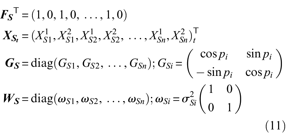
In Equation (11), the subscript i indicates the number of periods considered. An oscillation is decided by amplitude
The AR component describes the relationship between the current output and the n-order historical outputs. The previous n-order
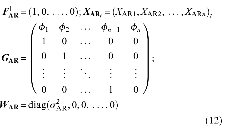
In Equation (12), the subscript AR refers to the auto-regressive feature. Once three-block components are integrated, the synthetical observation function is obtained as:

Sequential updating
In this part, the Bayesian updating process for system variables
Once the variables
Another key step of BDLM is to update the variables


The entire process is shown in Figure 4. If current information
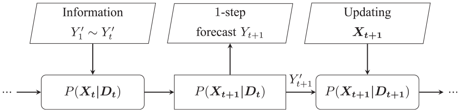
BDLMs updating flow chart.
Model parameters estimation
The final problem is how to calculate the arguments
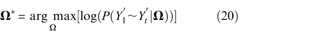
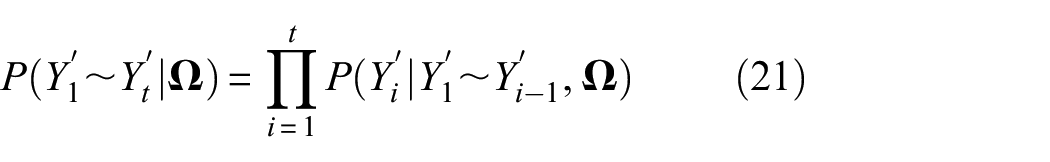
Equation (20) is the objective function, which aims to maximize the joint probability density of observations (Equation (21)). Any optimization algorithm, 52 such as batch gradient descent, can be implemented to search for the optimal solution. The termination criterion is based on the log-likelihood value as follows:
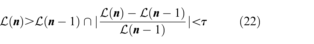
where
Partially observable Markov decision processes
This section aims to establish a sound decision framework to plan optimal maintenance actions based on the information from the SHM. The POMDP model is employed, which is a well-suited model for sequential decision-making problems operating under partial observation and an uncertain environment.
Discrete model
A traditional POMDP can be formulated by 7-tuple arguments
The challenge in POMDP is that the structural state is hidden. To handle this, we need to speculate the state distribution conforming to the Bayesian theory. A pertinence parameter referred to as the belief state vector
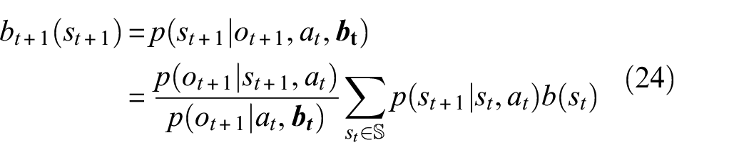
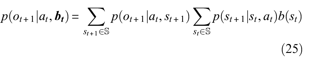
where the denominator
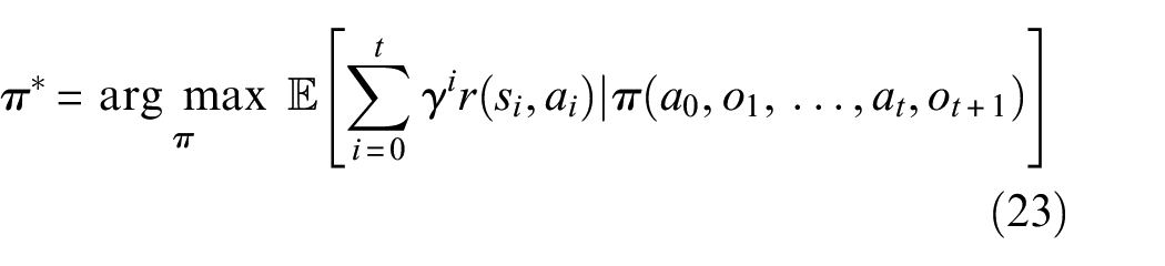
Additionally, the hidden state
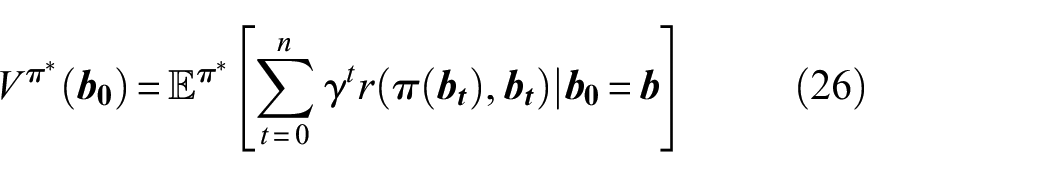
where Equation (26) is defined as the value function of belief point
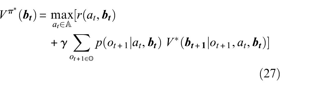
Equation (27) contains two parts, instantaneous reward and expected belief point value after being transferred
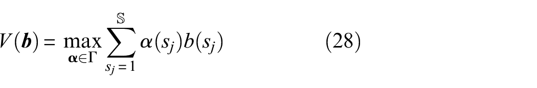
Through Equation (28), the belief point value is simplified as the probability of state
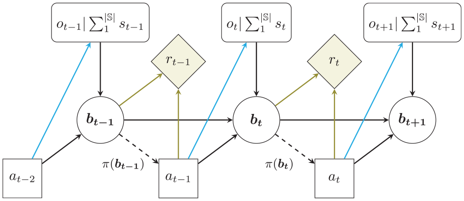
A schematic illustrating the POMDPs transference to belief-MDPs. The additional consideration is the probability of observation in each possible state.
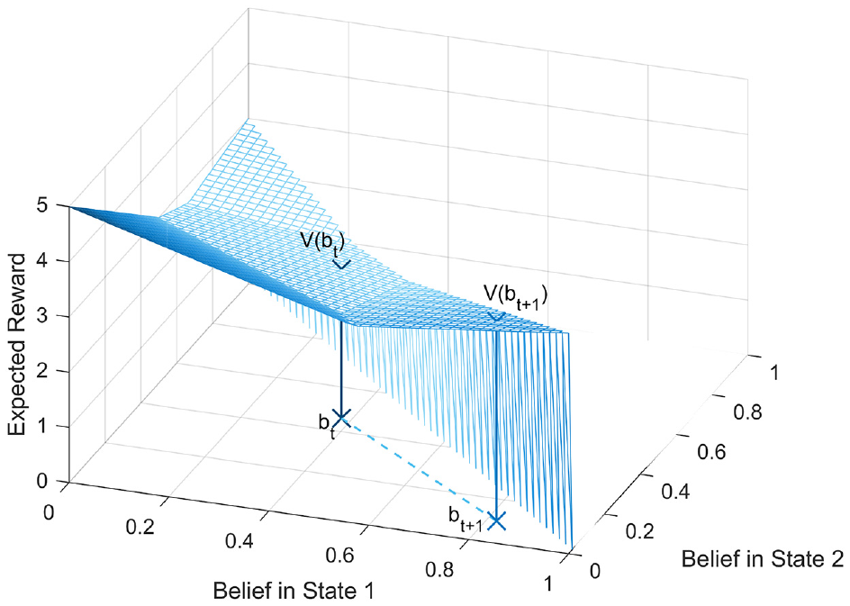
The solution process for three-dimensional POMDPs. The policy is represented by the multiple planes. The belief point value change from
Importing Equation (28) into Equation (27), the belief value updating function (29) is derived as:

In optimization, the above equation is named the BACKUP operator. An alternative pattern that facilitates programming in computer language is written as:
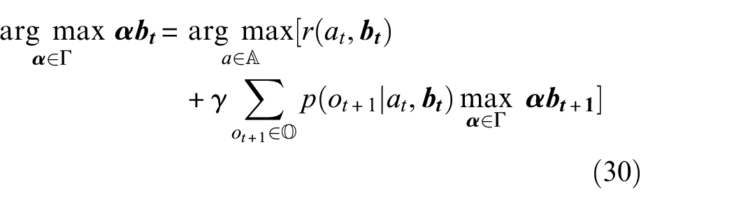
Notably, Equations (29) and (30) imply that each value coefficient
Continuous observation model
To embed BDLMs into the continuous observation POMDPs, the Gaussian mixture model (GMM) is employed to express the distribution associated with the prediction. It is well known that an arbitrary distribution can be divided into finite Gaussian distributions
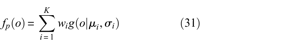
where K is the number of distributions in GMM. Once the PDF of the fatigue cycles

Then, the observation item
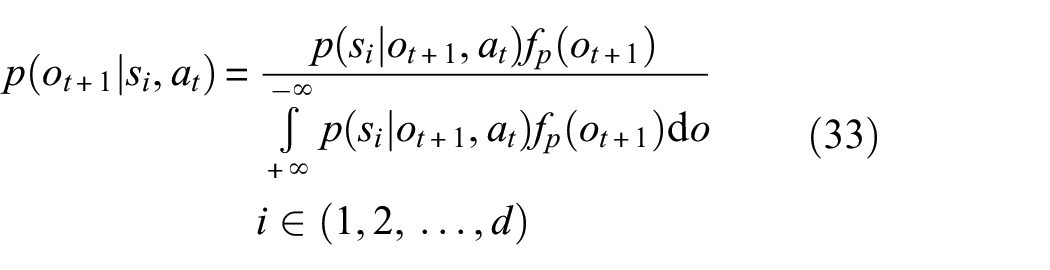
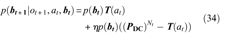
Another discrepancy between POMDP and the model in this study is the hidden state transition. Generally, POMDP assumes that the state degradation only relies on the prior state probability transition matrix. The observation is utilized to detect the current hidden state since the measurements will not affect the results. However, these two assumptions are not consistent with the practical component-level management incorporating the SHM system due to the following aspects. As the fatigue problem intrinsically contains high uncertainty, the condition of the component estimated by monitoring data is a probabilistic distribution rather than confidence about the state. In addition, the prior state transition matrix established by the inspected database reflects the generally deteriorated behavior of the similar component. For structural-level management, this roughly statistical model may be acceptable. But in component-level management, this approximation could induce large discrepancies with specific component deterioration. Otherwise, all the components in the bridge can share the same maintenance strategy, which is contradictory to the component maintenance in different locations of the bridge, load cases, and environment. Thus, the concept that the state transition depends on the posterior matrix is proposed. The confidence factor
Point-based algorithms in solving POMDP
To enhance the calculation efficiency, the point-based algorithm is proposed to alleviate the complexity in POMDP by avoiding the exponential increase of
However, the continuous observation space could cause other issues when utilizing point-based algorithms to sample the representative belief points. The lossless partitioning of the observation space could induce large observation spaces that need to be considered in POMDPs. To alleviate the complexity of observation spaces, various online solvers33,37,38 are developed, which use heuristic search in conjunction with branch-and-bound pruning to construct a look-ahead decision-making tree. Through interleave planning and plan execution, online solvers use the forward sampled scenarios to estimate the current belief value and decide the single best action for the current state. Although the online solver can dramatically decrease the computation, the solution achieved often falls sub-optimal. To obtain the optimal or near-optimal solution, the off-line solver needs to be employed, in conjunction with the algorithm which can “slim” the representative belief points. Therefore, by the consideration of the POMDPs features in infrastructure management, an efficient discretization strategy is proposed in this paper. Two characteristics in structural maintenance are utilized, (1) Generally, the consequence of failure is unacceptable in structure. Hence, the cost of failure state has high orders of magnitude compared with other states. (2) All the state transition matrix is unit-jump upper triangular matrix as indicated in Equation (5), except the replacing action. The mathematical property that the arbitrary value function
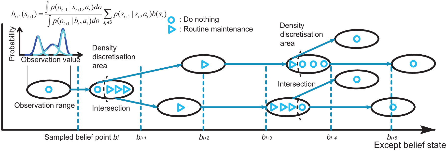
Adaptive discretization strategy in representative belief points sampling.
For the welded details, the observation in SHM is the number of stress cycles. Since the stress cycles are quantified as the unit-jump upper triangular matrix, the belief state is also monotonically increasing with the number of cycles. Hence, once it defines the belief state range corresponding to the same maintenance action in the optimal policy, the continuous observation that affects the belief state distribution in this range can be aggregated.
Illustrative example
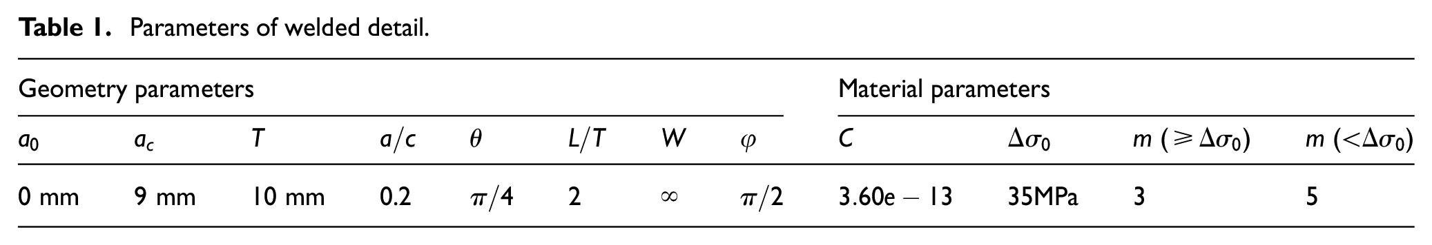
The fatigue details in bridge are studied to demonstrate how to plan the optimal maintenance strategies based on long-term monitoring data. To possess the real-time condition of the bridge, a dynamic SHM system was installed which includes weldable foil-type strain gauges. Major strain transducers are attached to components prone to fatigue. In this paper, since the methodology is concentrated on individual component management, the most vulnerable fatigue joint is selected which experiences the maximum stress range. Figure 8 marks the site of sensors which is fixed under the top flange of the box girder. This detail connects to the top flange plate through the U-welded joint. In this paper, the parameters of welded detail are listed in Table 1. The material arguments (F2 class steel) C and m are determined by the BS-7910 code and fatigue experimental results. 38
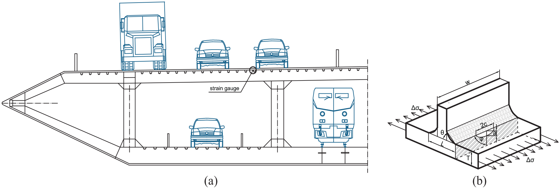
Welded detail monitored in the box girder. (a) Marks the welded joint location and traffic and (b) Shows the geometry of welded details.
Parameters of welded detail.
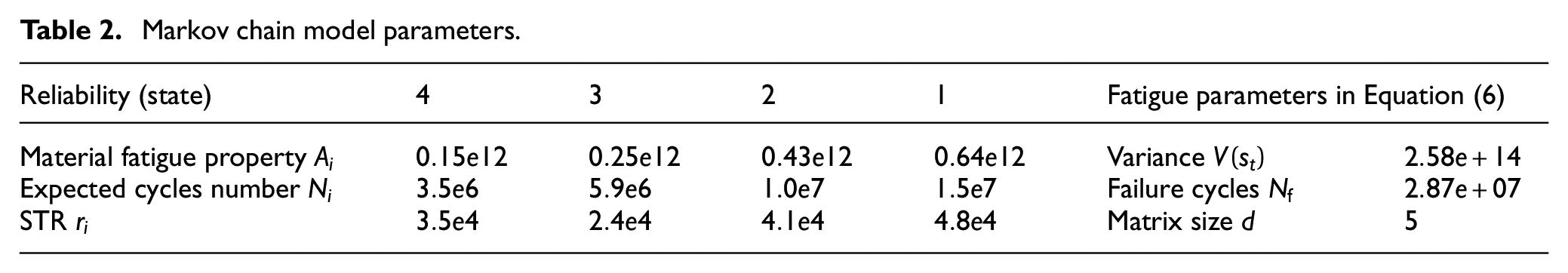
It should be noted here that the rate of crack propagation approaches infinity at the end of the failure phase. Since fragile behavior is unacceptable in the serviceability limit stage, conservative state thresholds need to be set. Herein, the states related to reliability are defined as infinite, 4, 3, 2, 1, based on the standard
49
proposed. State 1 refers to the intact state whose no cracks are possible to detect, while state 5 implies the potentially hazardous state at the onset of fracture. The fatigue properties of F2 class steel
Markov chain model parameters.
Corrosion parameters.
Data processing
The intensive sampling reproduces the original waveforms of the measurands, especially for extreme points. The representative measurements are shown in Figure 9(a), which has three characteristics: First, the strain pulses have a significant decrement from 1:30 am to 5:30 am as the train ceases its service during this period. It can infer that the strain pulses caused by the train are much larger than the vehicles by contrasting the amplitude of strain in daily strain time history. Moreover, the overall drift of strain is strongly synchronized with the temperature variation. However, the temperature strain does not produce stress in this welded detail because no constraints are in the strain direction. To separate temperature strain from the original signal, the maximal overlap discrete wavelet transform is used. This algorithm can decompose the signal into kth different frequency bands. Each band only contains the frequency that belongs to
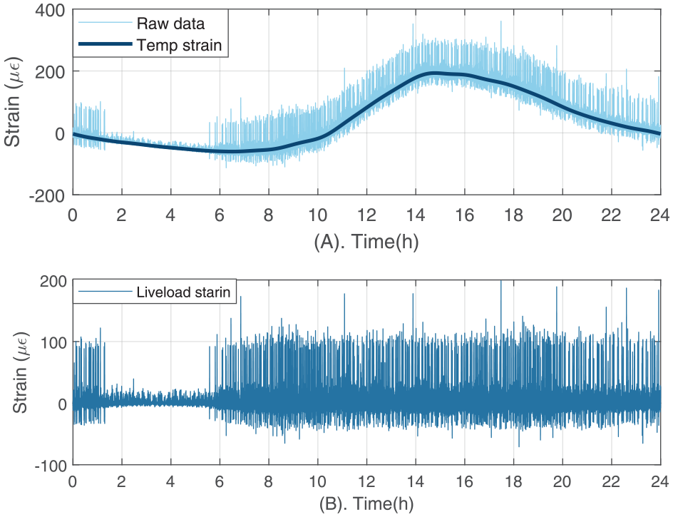
Typical daily strain spectra. The upper figure displays the temperature stain hidden in data. The lower picture is the live load strain.
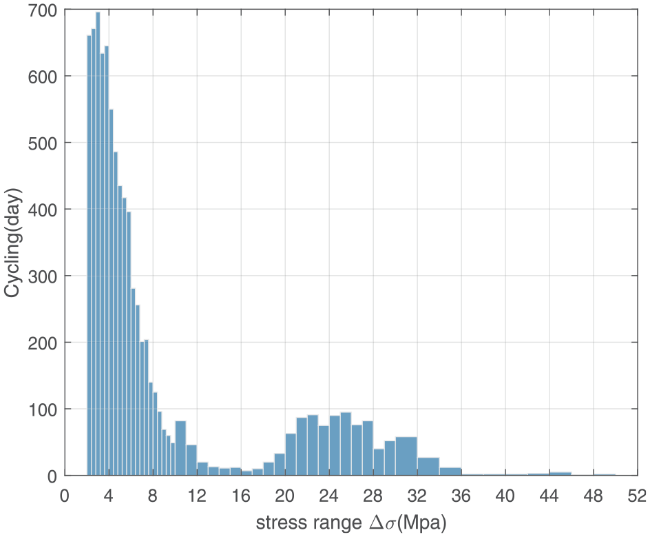
Stress spectra histogram. The different intervals are implemented based on the BS5400 recommendation.
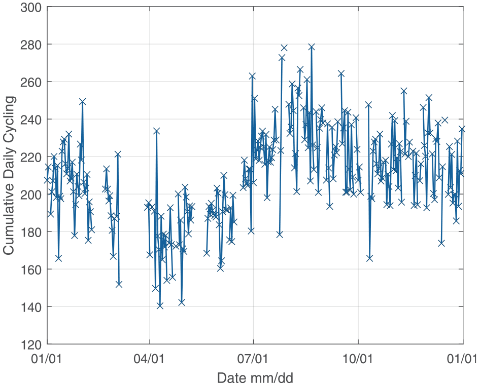
Whole year cumulative daily cycle. The fluctuation means the external impacts have randomness.
BDLM establishing
BDLM is constructed based on the daily stress cycling data in 2017, as Figure 11 shows. As mentioned before, the BDLM contains various block components where each block reflects one characteristic of data. The predicted model establishment is to attempt the different combinations of blocks to find a model that matches the data in Figure 11 with maximum likelihood value and acceptable error. Four representative BDLMs are assessed and listed in Table 4: (a) the AR model (
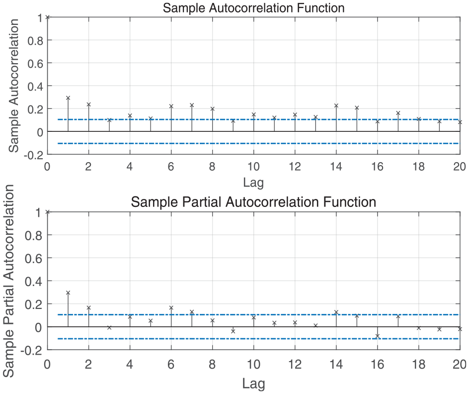
ACF and PACF in the AR blocks. The upper plot demonstrates lag reduced to zero. The lower plot shows a lag decrease to zero after AR(1).
BDLMs model parameters.
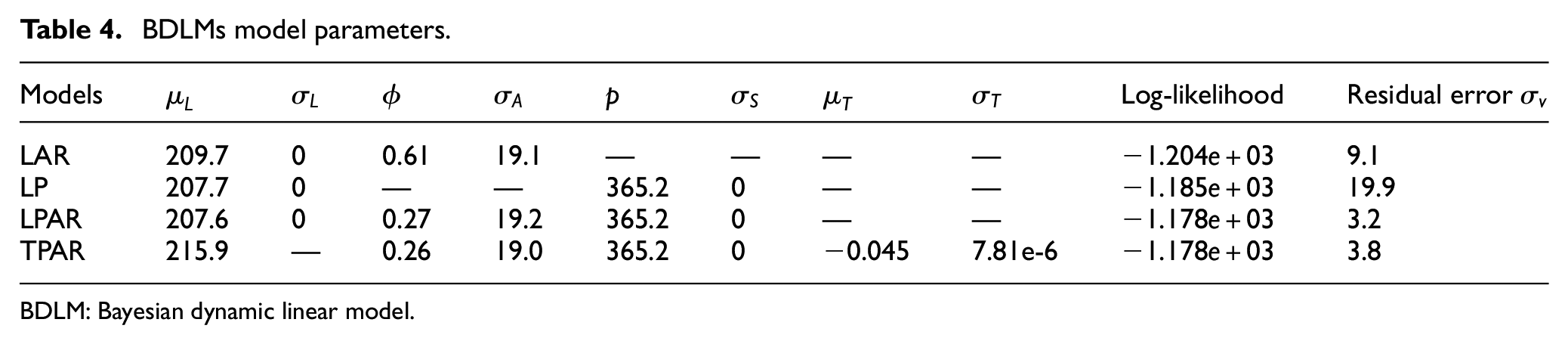
BDLM: Bayesian dynamic linear model.
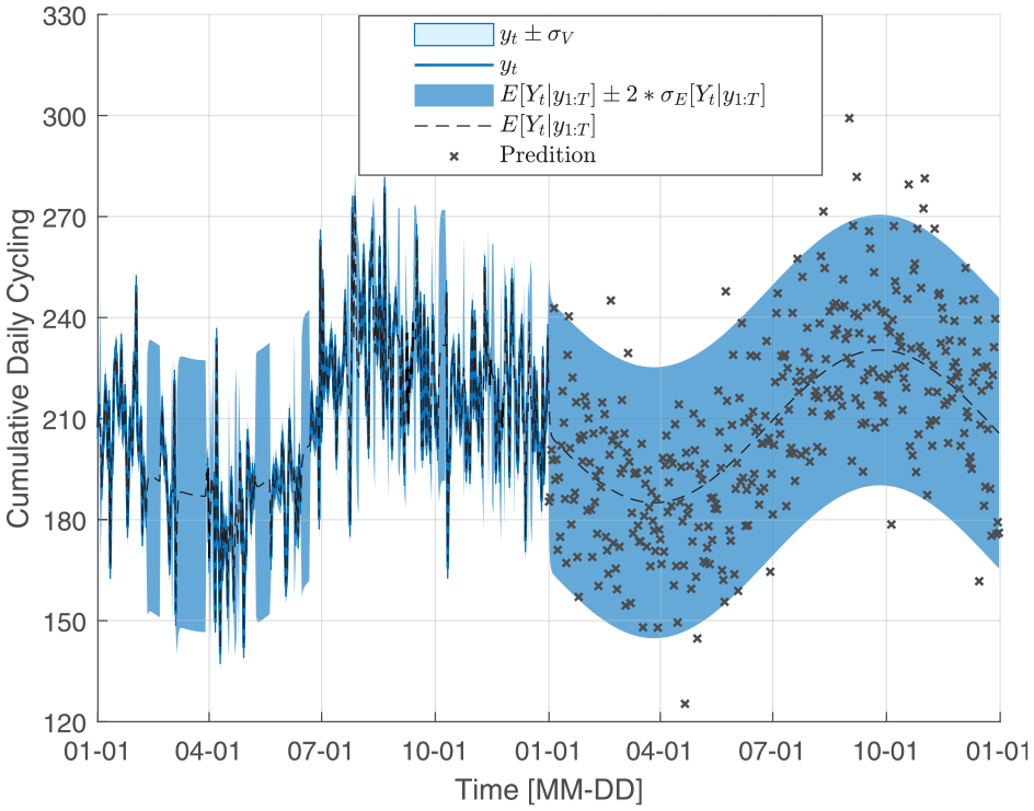
BDLMs for cycling forecasting. The light blue area is the two standard deviations intervals. The black dash line indicates the expected value development.
Management model establishing
This section describes how the continuous POMDP is established for bridge welded details management. The aforementioned methods, such as the Markov chain model for fatigue, BDLM for prediction, and GMM for observation are integrated into continuous observation POMDP to develop a comprehensive management system based on monitoring data. POMDP includes 7-tuple arguments
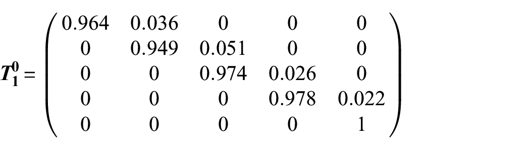
The corrosion will accelerate the deterioration of welded joints at three different rates. In phase 1, the accumulative exposure time is assumed less than 15 years and the corrosion accelerates the degradation 1.8 times. In POMDP, this acceleration coefficient is quantified by discounting the parameter of STR
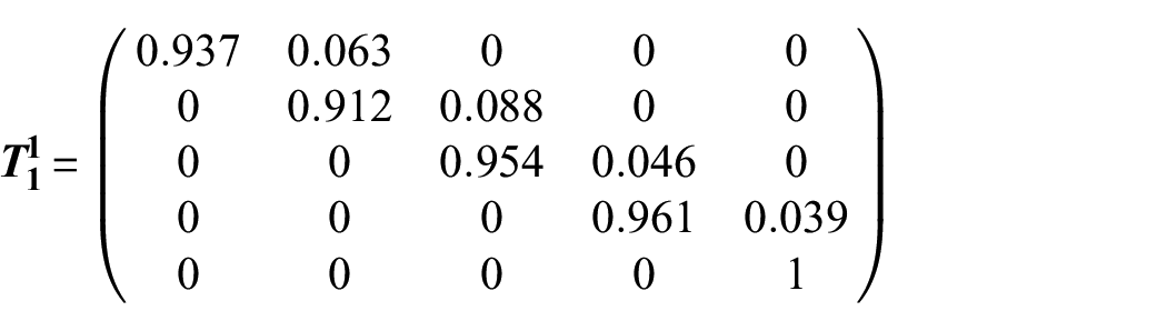
For phase 2, the joint is cumulatively exposed to an erosive environment for 15–30 years, and the accelerated coefficient is assumed as 2.6. For phase 3 (>30 years), this value increases to 3.4. The “Descaling and Painting” action shares the state transition matrix
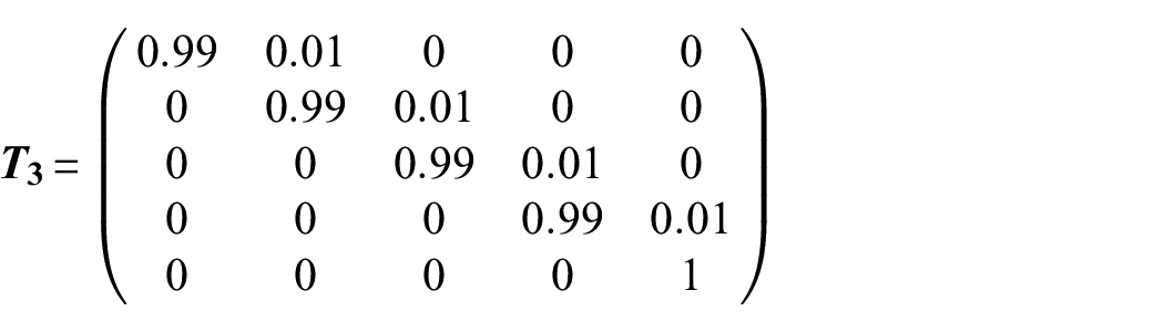
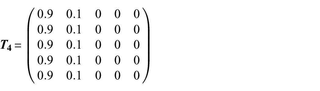
The state transition matrix
The observation parameters in continuous POMDPs are evolved from the probability matrix to the probability density functions. After the BDLMs are established, a stochastic observation value

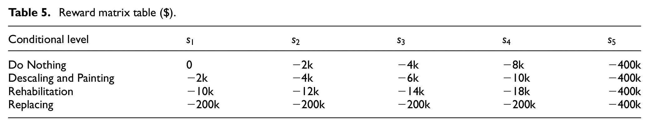
It should be mentioned that the different maintenance actions also affect the scope of observation results. When the welded joint has been cumulatively exposed to the erosive atmosphere for t years, the possible distribution cycling impacts during a time step are amplified as
Reward matrix table ($).
Results and discussions
Before gaining further insight into the maintenance behavior in optimal policy, the characteristics of modified POMDP will be emphasized again because these concepts are commonly overlooked and significant. It is worth noting that the conventional POMDP assumes that the hidden state transmission only depends on the prior state transition matrix
To illustrate how the welded joint degradation, the expected belief state deteriorated curves based on the prior state transition matrix and stress cycles from observation are separately plotted in Figure 9. Afterwards, the belief state evolution is obtained based on the posterior transition matrix
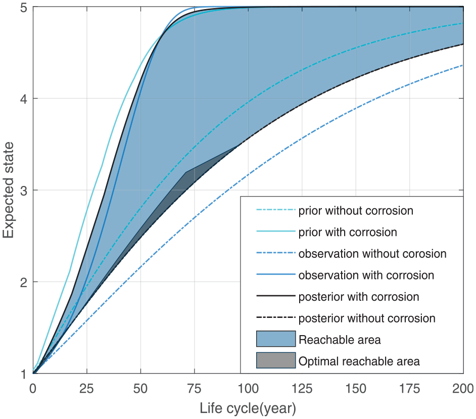
A schematic of component expected deteriorated curve. Notice that the dash-dot line refers to steel with perfect painting protection. The solid line is the deterioration in natural corrosion. The blue area B is the belief reachable space. The dark gray area
According to the reward parameters in Table 6, the comparison between the SARSOP algorithm and proposed discretization strategy in Appendix A is listed in Table 6. Since the maintenance fees will dramatically affect the optimal management behaviors, the sensitivity of price is studied by altering the reward parameter
Solver comparison table.
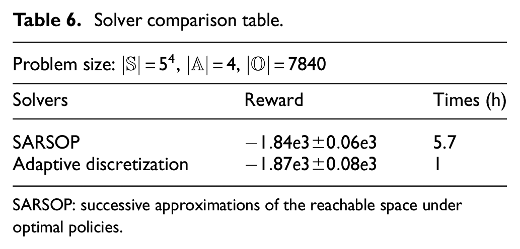
SARSOP: successive approximations of the reachable space under optimal policies.
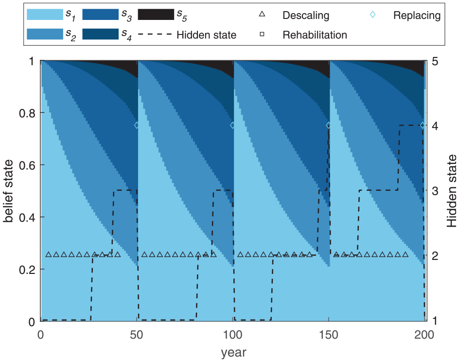
Policy realization of welded detail management. “Rehabilitation” is not adopted as an uneconomical action (10 k$).
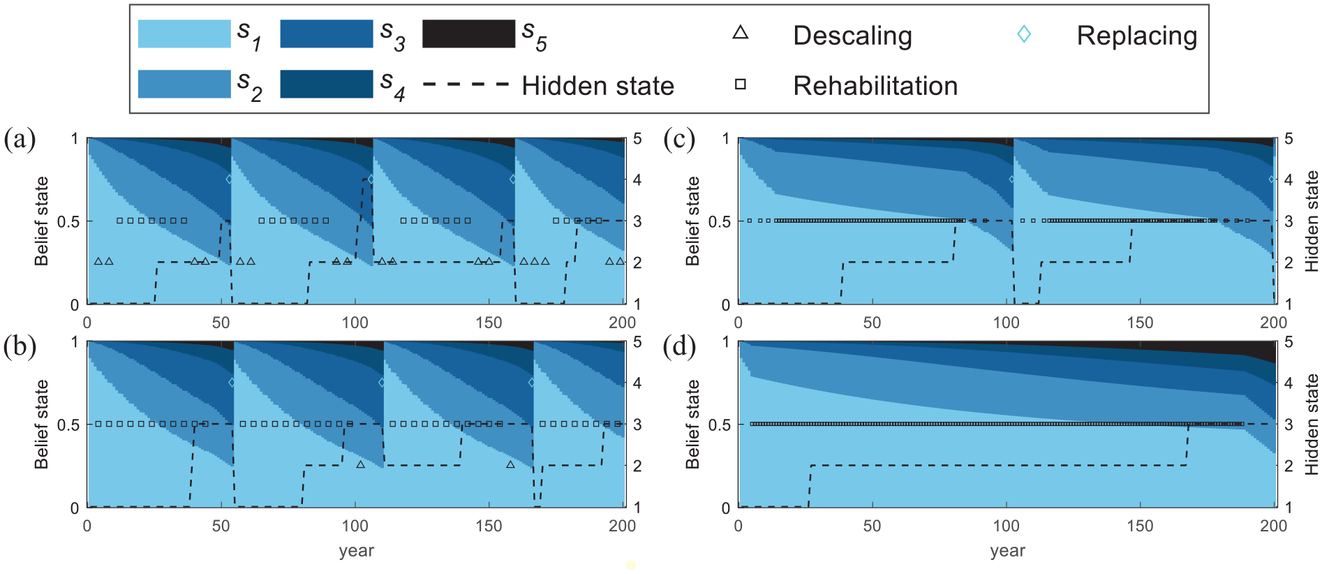
Policy realization of welded detail management with economical “Rehabilitation” action. With the decrement of “Rehabilitation” cost, the adopted frequency of this action has significant growth: (a) ``Rehabilitation'' cost is –5, (b) ``Rehabilitation'' cost is –4, (c) ``Rehabilitation'' cost is –3, and (d) ``Rehabilitation'' cost is –2.
The effects of cost performance in infrastructure management are investigated. The change in optimal maintenance strategy is observed when the cost of “Rehabilitation” is decreased. For the case that the cost of “Rehabilitation” decreases to −5, it will first be adopted in the mid-life time of the component, as shown in Figure 16(a). This behavior can be explained by the feature of the prior state transition matrices. In a welded detail naturally degradation (“Do nothing”), the capability of the component to maintain state 2 is the weakest (
The different maintenance actions present a competitive and complementary relationship based on their cost performance. To illustrate the effect of the cost-performance on the optimal maintenance policy, the concept of the “barrel effect” is utilized to present the competitive and complementary relationship among different interventions (Figure 17). When the maintenance utility (
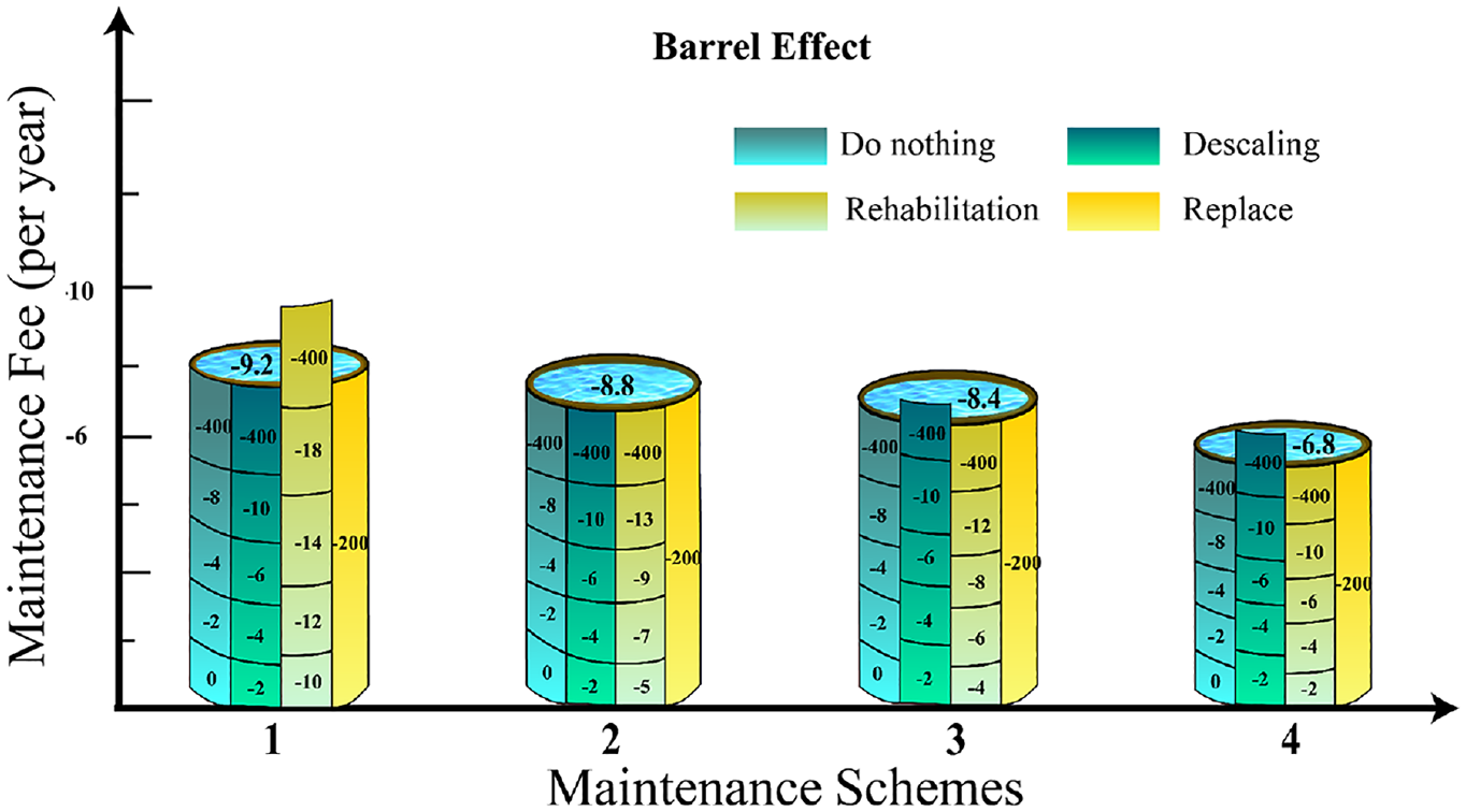
Barrel effect in decision-making. The value in the board denotes the cost of action in the different states according to Table 5.
However, the continuous POMDP has some limitations in application. The computation requirements considerably increase with solving large discretization observation spaces. For a welded joint, a computer equipped with an AMD 3900X and 64 GB memory still needs 1 hour to converge to the optimal solution. For large multi-component systems, individual component failure may not significantly affect the reliability of the entire structure. It requires the model to consider the synergy effect of component degradation act on structural safety. The offline solver cannot be applied to this scenario as the state and action spaces dramatically increase for the system-level management. The online solver, such as Actor-Critic, can alleviate the computation for optimal policy searching, but it cannot tackle the time-varying problem. Future work in sequential decision-making for complex engineering systems includes using dedicated deep reinforcement learning methods to solve the non-homogeneous deterioration problem and explorative training algorithms to ensure the model convergences.
Conclusions
A comprehensive decision-making framework for addressing the intelligent life-cycle management based on a real-world SHM system is presented in this paper. To realize this framework, the continuous observation POMDP is chosen as the theoretical foundation on the basis of its capability of formulating optimal sequential decision-making under stochastic environments with uncertain action outcomes and noisy observations. Through the Markov chain, the fatigue process is quantified as the discrete state transition in POMDP, which provides an alternative way to assess the condition of welded details based on long-term monitoring data. Further, to forecast the cumulative stress cycles of welded details in the life-cycle, the BDLM is used on the basis of its mathematical properties for a flexible combination of different blocks to characterize the data features and uncertainty in dynamic responses. Finally, based on the characteristic of infrastructure management, this study demonstrates the value function is concave and monotone decreasing with the expected belief state increasing. Using this property, an adaptive discretization strategy is designed to efficiently compute the optimal or near-optimal policy for continuous observation POMDPs.
A constructive concept about state transition in POMDP is proposed in this paper. The hidden state degradation is not merely reliant on the prior state transition matrix because stationary matrices cannot reflect the dynamic environmental evolution and uncertainty in external impacts. The state transition is determined by the posterior matrix which simultaneously considers the prior state transition matrix (general law) and observations (actual situation). According to the statistical results of maintenance behavior on a minimum budget constraint, the following specific conclusions can be drawn: (i) In infrastructure management, three factors will significantly affect the maintenance policy in the life-cycle: maintenance utility, deterioration rate, and cost of action. The optimal solution is to find the trade-off between long-short-term utility and cost. (ii) The available maintenance actions present a competitive and complementary relationship based on their cost and utility. The decision-making follows the “barrel effect,” which means that maintenance action with low cost-performance is the longboard and it would not affect the barrel capacity (cost). (iii) When a welded detail approaches the end of its lifespan, interventions to extend the lifetime are uneconomical. The “Do nothing” action is executed until replacing the detail to save the cost as much as possible.
Footnotes
Appendix A
In this part, we introduce how to incorporate the properties of infrastructure management to aggregate many observation domains, effectively decreasing the complexity of observation space. Since the deterioration of the component is a slow process, the upper triangular matrix with unit-jump, such as Equation (5), is recommended to represent this process.
62
Each STR (
The proof of this property proceeds by induction. If
Since the failure state cost is much larger than others
With the definition of the state transition matrix, we primarily focus on the quantity in Equation (37). Since the
Two mathematical characters could be summarized from Equation (39). First, in real-world infrastructure management, the condition of the component would gradually deteriorate before the replacement. Therefore, the value
In continuous observation POMDPs, the rich observation spaces pose heavy computation for a standard solver that is required for explicit enumeration of the observations, since it needs a lossless discretization observation space.
35
However, explicit discretization is difficult in SHM since the distributions of sensor readings are dynamic altering with interaction with external factors. Back to the POMDPs, the solver is to find the upper boundary line of the value function
In infrastructure management, replacing action is equivalent to resetting the POMDPs, and the boundary of this action is defined in steps 4–5. The approximate discretization of continuous observation can reduce the computational time, but it may cause another issue as Figure 18 shows. The value coefficient
Declaration of conflicting interests
The author(s) declared no potential conflicts of interest with respect to the research, authorship, and/or publication of this article.
Funding
The author(s) disclosed receipt of the following financial support for the research, authorship, and/or publication of this article: The study has been supported by the Research Grant Council of Hong Kong (project no. PolyU 15219819 and PolyU 15221521). The support is gratefully acknowledged. The opinions and conclusions presented in this paper are those of the authors and do not necessarily reflect the views of the sponsoring organizations.