Sage Journals: Discover world-class research

Abstract

This paper presents the design and experimental realization of a cooperative radar network for structural health monitoring (SHM) of wind turbine blades. For this purpose, 40 FMCW (frequency-modulated continuous wave) radar sensors operating from 58 to 63.5 GHz have been installed in a 31-m-long blade during manufacturing. A subset of 10 sensors is material-embedded in the core material of the blade, and the remaining thirty sensors are placed inside the blade on an inner rotor blade surface. The sensors are distributed over the entire blade based on previous high-frequency electromagnetic simulations. A full-scale fatigue test has been performed under controlled laboratory conditions. In addition, holes have been drilled into the blade by hand to represent a well-defined and relatively small damage. During the experimental campaign, measurements from the complete radar network have been transferred to a base station through a wireless communication link. Finally, it was demonstrated that fatigue as well as artificial damage could be detected accurately using the proposed damage indicator (DI) approach.

Keywords

Radar-based SHM wind turbine blades fatigue testing damage detection radar sensor network

Introduction

The renewable generation of electrical energy from wind is of great importance for supplying households, mobility, and industry. In order to cover the immense demand and to replace conventional energy sources, more and larger wind energy plants have been built leading to increased cumulative wind power worldwide.¹ The inspection and maintenance of wind turbines especially in rural and harsh environments are challenging, time-consuming, and costly.² For these reasons, a continuous and automated monitoring in the form of a structural health monitoring (SHM) system is of great interest concerning economic and safety aspects.

The blades are critical components of a wind energy plant given by their large dimensions and complex geometry. Recently, Sun et al.³ summarized in situ monitoring approaches of wind turbine blades from the past years. These approaches range from vibration-based methods⁴ and acoustic emission measurements⁵ to optical⁶ and electromagnetic sensing such as thermography.⁷ In addition, radar methods have been proposed that monitor the blades remotely from the ground^8,9 or from the wind turbine tower.^10,11 A major drawback of such external monitoring methods is that they constantly have to deal with a changing sensor perspective caused by rotor blade movement. This drawback can be overcome by integrating the sensor system into the moving blade. Radar-based methods offer a variety of advantages. Compared to guided ultrasonic waves,^12,13 no mechanical waveguide is required, and no higher order wave modes exist that usually lead to complex ultrasonic signals. In addition, electromagnetic waves propagate in air over large distances with limited attenuation, which is advantageous for structures with large cavities, such as wind turbine blades. An active radar transmitter and receiver enable inspection without structural loading which is required in vibration-based and acoustic emission techniques.

The present work aims at an embedded radar network permanently installed in a wind turbine blade operating in the 60-GHz frequency band. Figure 1 illustrates the concept consisting of multiple low-power and low-cost radar sensors spatially distributed over the structure that are able to communicate with each other and a base station through a wireless data link.¹⁴ Damage detection is based on a local or centralized analysis of the radar signals. The network is cooperative in terms of coordinated measurements of radar sensors to prevent electromagnetic interference. The sensors can be powered through energy harvesting as done by solar foils.

Figure 1.

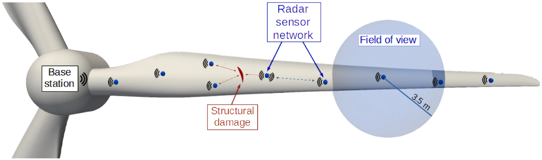
Schematic representation of the embedded radar network in a wind turbine blade showing individual radar sensors, their field of view (about 3.5 m each), damage triangulation for damage assessment. and the wirelss data communication link with the base station.

A critique from Sun et al.³ about electromagnetic monitoring methods is the susceptibility of electromagnetic radiation to interference. By integrating the sensors into the blade, the influence of interference sources is minimized because the distance to the target is reduced to a minimum and environmental influences such as temperature or humidity have a reduced impact. Since the sensors in the blade only have to cover a limited field of view as well as short distances, the output power can be in the order of milliwatt and hence much lower than that of the electromagnetic radiation of a mobile phone.¹⁵

The author’s previous work showed the damage detection capability at 60 GHz for typical rotor blade defects on coupon level.¹⁶ In addition, research has been conducted on the optimal placement of the frequency-modulated continuous wave (FMCW) radar sensors in the rotor blade through high-frequency electromagnetic simulations.¹⁷ The final sensor distribution in the 31-m-long blade is shown in Figure 2. With this sensor distribution, a large part of the rotor blade is covered with triple redundancy to compensate for individual sensor failures. In a few selected areas, there is less coverage (1-fold or 2-fold) due to limitations in the number of sensors.

Figure 2.

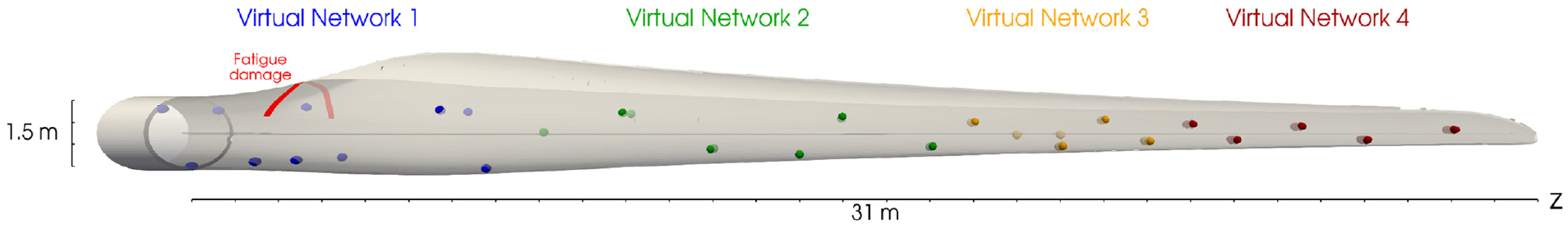
Rendering of the 3D rotor blade model showing the radar sensor distribution, their arrangement in virtual networks sharing the same base station (color-coded), and the position of the fatigue damage (red).

The novelty of the paper is to develop and validate an embedded radar network consisting of multiple low-cost radar units to achieve a full-coverage monitoring of a rotor blade. The approach is examined in a full-scale fatigue test with a 31-m-long rotor blade for its functionality and applicability. This is vital, as the scope and realism of laboratory tests is often criticized.³ The developments include a method for embedding sensors in the core material of the rotor blade to protect the sensors from environmental influences and to demonstrate its proof of concept. Moreover, signal-processing techniques have been developed to assess structural conditions with a damage indicator (DI) approach.

System description

Radar sensor description

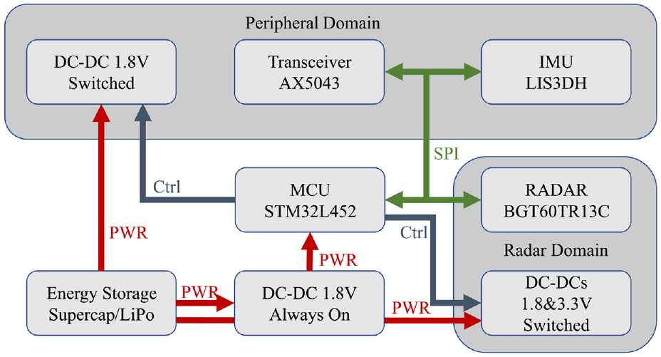
Each sensor node in the network consists of a 60-GHz radar, sub-GHz communication, inertial measurement unit, power supply, and a controlling microcontroller. A block diagram of the system is presented in Figure 3. The system is optimized for ultra-low-energy consumption and extended time periods without an external energy supply. The network is split in two different sensor types which differ only in energy supply and overall form factor. The components used and firmware deployed is identical. One system is designed for embedding in the blade material during production, whereas the other system is intended for mounting to an inner surface inside the rotor blade (retro-fit solution).

Figure 3.

Block diagram of a sensor node.

The embedded sensor variant uses a 1 F supercapacitor for energy storage and is intended to be supplied through solar foils from the outside, whereas the other system is supplied from the inside through wires. The latter uses a 560-mAh lithium polymer cell for energy storage. Both systems can thus react to a loss of external power, by reducing their duty cycle until power is restored.

The radar itself consists of an integrated 60-GHz FMCW radar, the BGT60TR13C by Infineon which is optimzed for presence sensing or gesture classification.¹⁸ The antennas are integrated in package and arranged in a 1-TX/3-RX configuration. Each RX channel can be measured individually. This allows the system to gain a broader view of its surroundings, as each RX-antenna’s pattern is affected differently through the embedding process.¹⁹ The maximum detection range is 3.5 m that was defined by the sampling rate $F_{ADC}$ of the integrated ADC (analog digital converter), speed of light c, and the slope S of the FMCW ramp:

d_{\max} = \frac{F_{ADC} \cdot c}{2 \cdot S} .

(1)

This ensures that a large enough area of the opposite side of the blade is visible to the radar. The microcontroller used for data acquisition and power management is a STM32L452 ultra–low-power MCU (micro-controller unit). The sub-GHz transceiver is an AX5043. The communication interface is described in detail in the following section.

The power supply is based on multiple DC–DC converters which are enabled and disabled according to the needed subsystem which they power. The MCU is continuously supplied with electrical energy, whereas the other peripherals are only powered for measurements or communication.

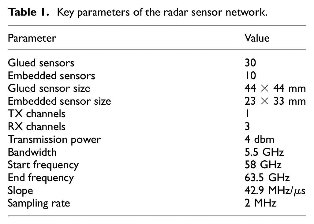
The FMCW sensors send out frequency ramps from 58 GHz to 63.5 GHz in a sawtooth pattern within a sweep time of T = 128 µs. The backscattered signal is measured in baseband with a sampling rate of 2 MHz, resulting in signals with 256 data points. In total, a series of 128 signals can be temporarily stored on the sensor node per channel. Table 1 summarizes the most important parameters of the radar sensor network.

Table 1.

Key parameters of the radar sensor network.

Parameter	Value
Glued sensors	30
Embedded sensors	10
Glued sensor size	44 × 44 mm
Embedded sensor size	23 × 33 mm
TX channels	1
RX channels	3
Transmission power	4 dbm
Bandwidth	5.5 GHz
Start frequency	58 GHz
End frequency	63.5 GHz
Slope	42.9 MHz/µs
Sampling rate	2 MHz

Wireless network communication

The proposed sensor system is optimized for ultra-low-power operation with measurements taking place every few hours. However, the highest possible amount of sensor data is desirable during fatigue testing. This data rate is mainly limited by the communication through the sub-GHz transceiver since the maximum achievable data rate is 125 kbps.²⁰ The effective data rate is further reduced by protocol overhead and the fact that multiple sensors shown in Figure 2 communicate with one base station simultaneously. These base stations consist of the AX5043 transceiver mounted on an STM32F767ZI-Nucleo board in an acrylic case as can be seen in Figure 4. The received data is then transmitted via Ethernet to a central computer.

Figure 4.

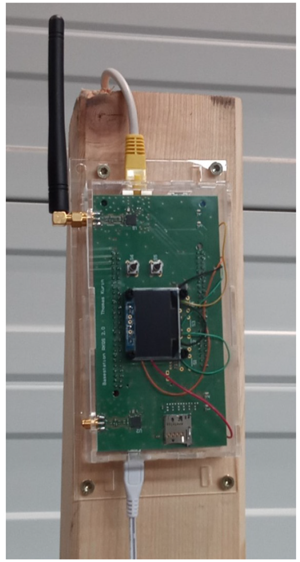
Photo of a sub-GHz base station in the test setup. In total, four base stations have been used.

As a fallback in case of potential sensor firmware updates or system reconfiguration, an OTA (over the air) boot-loader was implemented in the sensor firmware, which was triggered by an internal watchdog or a command from the base station. This allowed the base station to transmit a complete new firmware to the microcontrollers embedded Flash with reduced data rate for a better BER (bit error ratio).

The wireless communication uses a 2-FSK (frequency shift keying) modulation at 868 MHz. Each base station communicates at adjacent channels spaced 350 kHz apart. The FSK deviation for the data communication was 25 kHz and for firmware updates 4 kHz. As a complete radar data block consists of 576,000 bits, the theoretical achievable readout time was 5.76 s per data block. By splitting the data in packages of 190 bytes and overhead through CRC (cyclic redundancy check), counter and repeated preambles, etc., the total time from one sensor readout to the next was increased from the theoretical 5.76 to 14 s per RX channel.

Communication scheme

Radar measurements and wireless data communication are triggered through the base station to allow the most flexible network organization. In the present work, 10 sensors were grouped in a virtual network sharing one base station. This arrangement supports four parallel radar measurements in different regions of the wind turbine blade. The design of the virtual network accounts for maximum distances between active radar sensors to minimize mutual interference (see Figure 2).

The base station transmits a keyword as well as the sensor ID. When the sensor receives this key, it transmits the last measured radar data block and starts a new radar measurement. Then the base station can either continue communicating with that sensor or request another sensor to commence communication. To ensure a continuous measurement, all sensors were read out consecutively. If sensor data were corrupted or the sensor did not respond, that sensor was ignored, and the next sensor in row was read out. Every data block was CRC-32 protected.

Under extremely unlikely circumstances, the sub-GHz transceiver could get stuck in a loop and would not receive any commands. In that case, the system would perform a complete system reset if it did not receive any command data for a prescribed amount of time.

Experimental design

Rotor blade manufacturing with embedded radar networks

The blade in this work was manufactured in the facilities of the Fraunhofer IWES (Bremerhaven, Germany). A butterfly manufacturing process was used with two main molds for the suction and pressure shell and two separate molds for the spar cap and the web. The blade consists of dry non-crimp glass fiber (2,7t), PET foam (0,1t) and Balsa wood (0,1t) as core material, PU resin matrix system (1,5t) and 0,2t PU adhesive material for the bonding of web and shell components. The material handling was done by hand in a manual process chain. The fiber impregnation was realized by vacuum infusion process. Therefore, the molds were completely encased in a bag and the material got infused under vacuum conditions until the entire component was impregnated with resin. This was followed by a curing step at 60°C for 6–8 hr. After curing, the bonding process of the separate blade components was started. The web was glued into the suction side followed by the pressure side on top of the upper web foot and the suction side. The subsequent hardening step needed 16 hr at almost constant 60°C. After curing, the rotor blade was removed from the mold and transferred to the post-processing of the adhesive edges and the blade connection.

A manufacturing process for surface-mounted and material-embedded sensor placement has been developed. In total, 40 sensors were installed with 10 sensors directly embedded into the blade shell and the remaining 30 sensors as retro-fit solutions at inner surfaces of the blade. An example of a retro-fit sensor in a 3D-printed case is shown in Figure 5. A major challenge was to feed through the wires for the power supply of the 10 embedded sensors without any negative impact to the mechanical blade behavior. In addition to this, the actual manufacturing process should not be influenced to ensure transferability to industrial production. Therefore, it was decided to integrate the sensor in the 15-mm-thick core material. A notch was milled out in the core material for optimum shape adjustment, and beforehand, the radar sensor was embedded in a matrix with the same notch shape (Figure 6(a)). This enables an optimal form-fitting insertion of the sensor. The wires for the power supply were placed on the surface of the mold before starting the blade manufacturing, and they were protected from resin by a separate vacuum bag (Figure 6(b)). This was followed by the conventional layer structure placement whereby the wires had to be handled through the fabric layer by layer (Figure 6(c)). This happened until the core material was deposited (Figure 6(d)). The embedded sensor was placed there and connected to the wire (Figure 6(e) and (f)). Finally, a functional test of the whole radar network was carried out before the start of the fatigue test.

Figure 5.

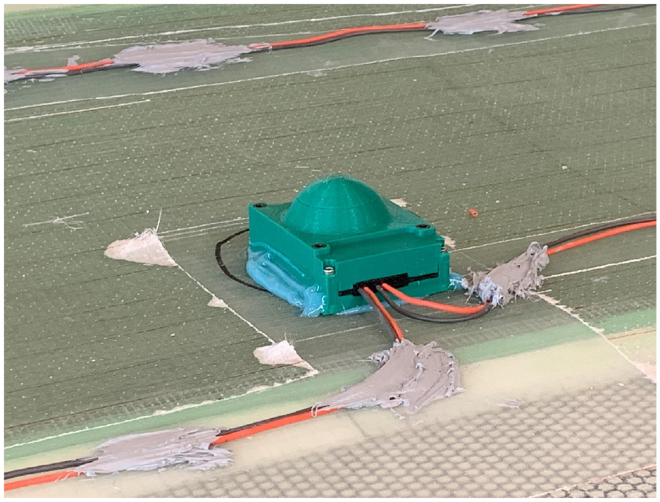
Surface-mounted retro-fit sensor inside of a 3D-printed plastic case that is transparent at mm-wave frequencies.

Figure 6.

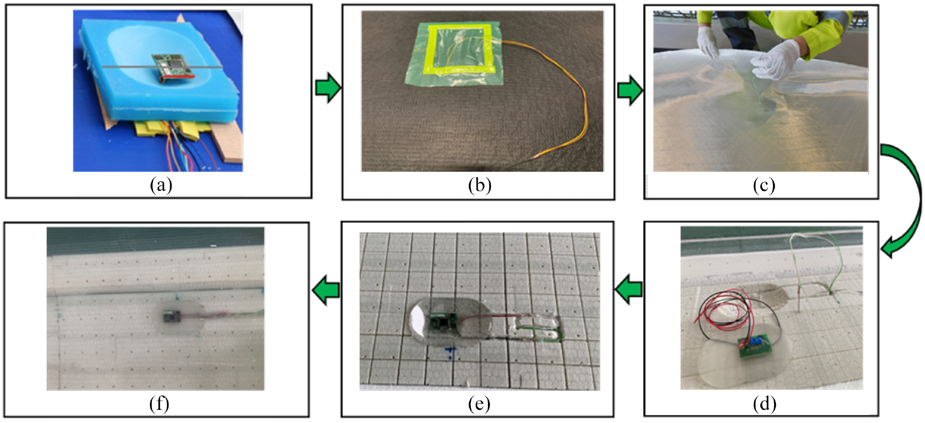
Documentation of the embedding process of radar sensors in the rotor blade during manufacturing. (a) Sensor embedding, (b) vacuum bag and wire positioning, (c) material & wire handling, (d) sensor after infusion, (e) wire connection and (f) sensor and core placement.

Description of full-scale fatigue testing

The rotor blade “IB30 rotor blade” was tested in an edgewise full-scale fatigue test in the 70-m hall of Fraunhofer IWES in Bremerhaven. Edgewise fatigue tests pose a special structural challenge and are generally considered more critical than flapwise fatigue tests. The test was performed according to the current state-of-the-art, referring to IEC 61400-23:2014-04.

The blade was attached to the test block with the pressure side up and excited at 1.61 Hz which is close to the system natural frequency using a ground-based hydraulic cylinder, attached to load frame no. 2 as can be seen in Figure 7. To optimize the bending moment distribution along the blade, four load frames were mounted on the blade as shown in Figure 7. The figure shows the test setup of the fatigue test and the number, the total mass, and the radial positions of the load frames. Adjusting the bending moment distribution with additional masses along the blade is mandatory to perform a reasonable fatigue test. The reason for this is the nonidentical curvature of the desired and the real bending moment curve. The masses increase the acting bending moment in the test from the mounting location to the root. This makes it possible to test each position of the blade sufficiently as well as avoid excessive overloading, as this would lead to premature failure. This approach corresponds to the proven procedure in certification tests.

Figure 7.

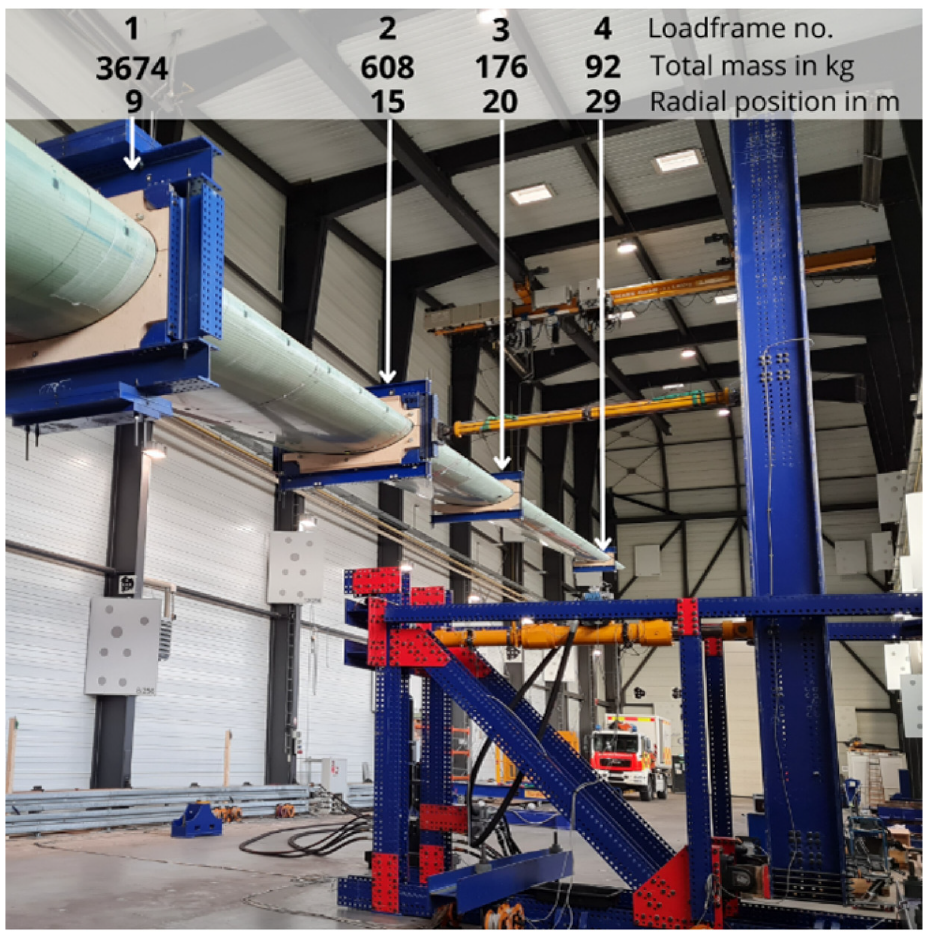
Rotor blade on the test block with four mounted loadframes and attached cylinder for excitation.

From previous experience with an identical rotor blade also tested by IWES, three load levels were planned to produce structural damage resulting from the fatigue test as opposed to a one-time static overload. 100% load level describes the condition at which it is assumed that the blade can withstand a long-term load without major damage. This state corresponds to the actual bending moment curve that occurs during the test with parameters 3531 kNm at radius 1 m (R1), 2334 kNm at 6 m (R6), 1295 kNm at 12 m (R12), 677 kNm at 17 m (R17), and 273 kNm at 22 m (R22). The load level increase has been implemented by enlarging the cylinder stroke at R12. Compared to this 100% load level, 400,000 cycles each at 102.5%, 106%, and 112% load levels were carried out. In the literature, fatigue damage is defined as “iterative deterioration caused by the cyclic loading of a component or material, which eventually leads to crack initiation and, shortly after, final fracture.”²¹ The fatigue mechanisms for fiber-reinforced polymer composites, a core material of wind turbine blades, are different compared to metallic structures given by the anisotropic and inhomogeneous material properties. The initiation and propagation mechanism of fatigue damage in such materials is a complex interaction of matrix cracking, fiber-matrix debonding, fiber breakage, and delamination between fiber layers.²² More detailed information about fatigue damage mechanisms is beyond the scope of this paper and can be found in research done by Shabani et al.²³ and Zuo et al.²⁴ These processes lead to a change in the dielectric properties of the material as well as structural changes with additional interfaces, and can thus be detected with the radar systems. In the present work, visual inspection has been performed periodically during the fatigue test for validation. Glue line cracks appeared in the trailing edge and delamination appeared at the root-side start of the pressure-side web starting at the 106% load level. The damages increased as the test progressed, but did not become structurally critical. Due to the absence of major structural damage, the load was further increased to induce major structural damage.

The intention of the test sequence was to cause several damage types, and for the last stages of the fatigue test, the load was increased to 117%, 122%, and 127% load levels and was maintained for several thousand cycles in each case. At 127% test load, a 1.5-m-long crack developed over approximately 20,000 cycles, running across the entire trailing edge at a blade length of 2.5 m in the transition region of the blade. This damage, shown in Figure 8, marked the end of the fatigue test after 1.25 million cycles.

Figure 8.

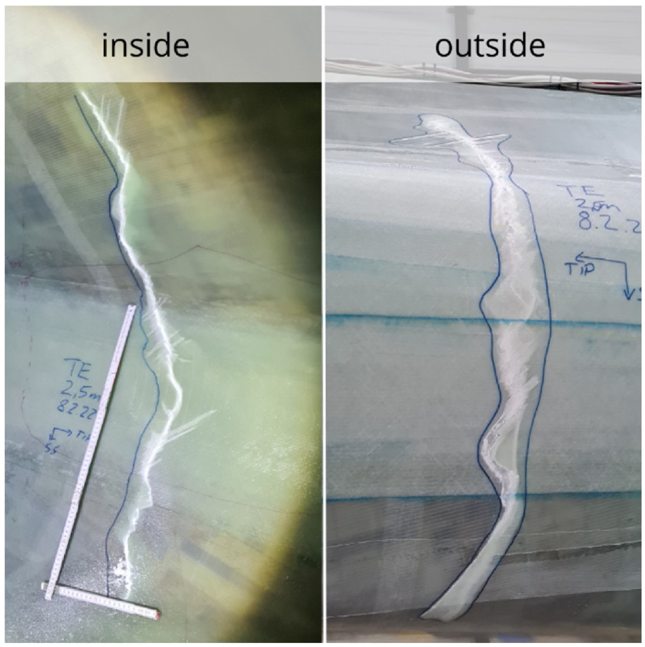
1.5-m-long crack from pressure side to suction side through the trailing edge of the blade (view from inside and outside).

A reference state is required in the proposed monitoring approach similar to other SHM techniques, such as acousto-ultrasonics or vibration-based analysis. The idea is to study relative changes in the signals with respect to a baseline condition and to evaluate such changes for damage assessment. In the present study, this reference state should be defined as simply as possible in order to remove potentially overlapping effects, such as temperature variations or loading, from the analysis and to obtain results that are as unambiguous as possible. The experiments on coupon level¹⁶ showed that structural loading during fatigue testing has a significant impact on the radar signals. This leads to the conclusion that measurements at different displacement of the rotor blade are not directly comparable, because the loading effect is stronger than the signal response from damage. For a reference-based SHM procedure, it is of utmost importance that the reference measurements for the intact structure as well as all further measurements, including a potential structural damage, are recorded under comparable conditions. A measurement in displaced state can only be used for damage detection on the basis of a reference with comparable displacement. To ensure such conditions for the present work, the measurements were performed on a static blade, for example, overnight, for intact and damaged conditions.

Results

Signal conditioning

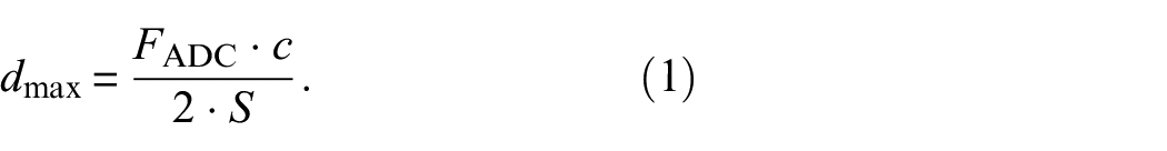
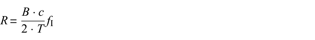
FMCW radar sensors typically mix the received signal with the transmitted signal to obtain a signal with distance-dependent intermediate frequencies $f_{I}$ . The raw time data of a mixed frequency ramp can be transformed by a Fourier transform into the frequency domain. This frequency domain spectrum contains amplitudes in dependence of the distance to the sensor. The corresponding distance axis can be calculated from the radar parameters via

R = \frac{B \cdot c}{2 \cdot T} f_{I}

with bandwidth B, speed of light c, and ramp duration T. The result is a radar signal, also called range profile, containing echoes from adjacent targets. In this work, we propose a differential SHM approach where range profiles are subtracted from those obtained during baseline conditions, that is, the intact state of the structure directly after production. In this work, we propose a differential SHM approach where range profiles are subtracted from those obtained during baseline conditions, that is, the intact state of the structure directly after production. This leads to a residual signal containing information about structural changes with respect to the pristine condition of the rotor blade. In the context of this work, the observed signal changes correspond to the fatigue damage in the blade.

Since most of the wave propagation happens in air and not in the dielectric rotor blade material, the dielectric properties of air have been considered in this work as an approximation. With the proposed differential monitoring approach, measurements from reference and damaged conditions are affected to the same extent so that this assumption is of minor importance.

The radar signals show a noticeable amount of noise in the time and frequency domains as depicted in Figures 9 and 10 for sensor 1 during the reference measurements. The figures show 10 consecutive ramps taken from a series of 128 ramps. The possible reasons for these signal variances are manifold and can arise from hardware, software, and their combination. Figure 10 indicates recurring ranges with almost no fluctuations. This makes timing problems unlikely and rather indicates hardware inaccuracies. This observation required a detailed analysis on the signal fluctuation prior to the fatigue test to ensure optimal signal conditioning that ensures the signal fluctuations are much smaller than the scattering response from damage.

Figure 9.

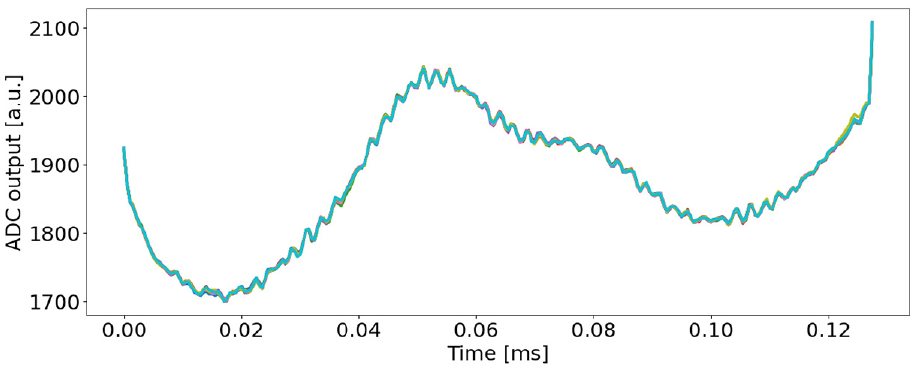
Raw time-domain radar data of 10 consecutive ramps of sensor 1 (intact blade condition).

Figure 10.

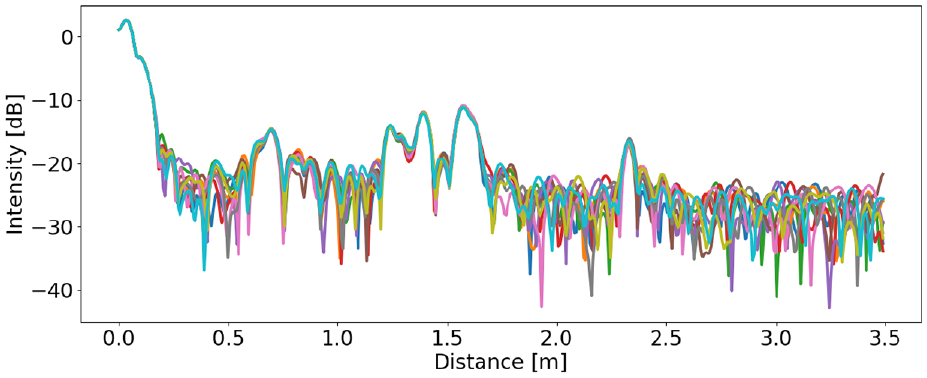
Range profiles of 10 consecutive ramps on a logarithmic scale of sensor 1 (intact blade condition).

In order to find a meaningful number of signal averages, two sets of measurements containing 4096 frequency ramps were compared. These measurements were performed with identical embedded radar sensors in laboratory conditions prior to the fatigue test. The data are preprocessed as described before, which means the Fourier transform is calculated for every ramp, and the ramps in the frequency domain are averaged. To evaluate the fluctuations, we calculate the maximum difference via

max {\frac{1}{n} \sum_{1}^{n} (s_{n, 1}) - \frac{1}{n} \sum_{1}^{n} (s_{n, 2})} .

between the first n ramps of the first measurement $s_{n, 1}$ and the first n ramps of the second measurement $s_{n, 2}$ . The result is shown in the top part of Figure 11. Since this may lead to a single high peak value, the sum over all signal differences is considered as well:

\sum {\frac{1}{n} \sum_{1}^{n} (s_{n, 1}) - \frac{1}{n} \sum_{1}^{n} (s_{n, 2})} .

Figure 11.

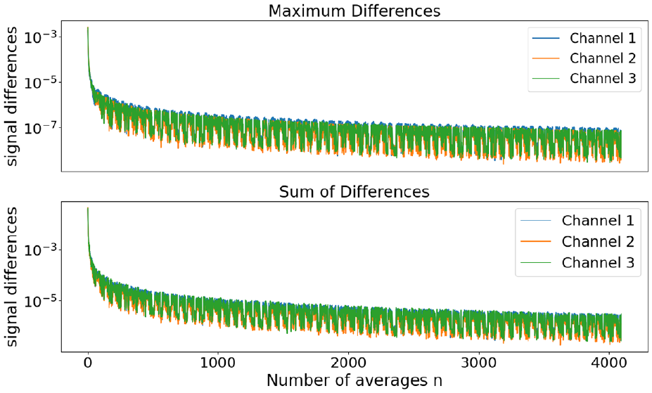
Analysis of the signal fluctuations as a function of the number of signal averages: n (top) maximum signal differences and (bottom) sum of signal differences.

The result is shown in the bottom part of Figure 11. The plots are of similar shape, and both considerations lead to the conclusion that signal fluctuations can be steadily reduced by increasing the number of signal averages. However, a higher number of signal averages also requires longer time for data acquisition and especially for wireless data transmission. Hence, a trade-off must be found, and the number of signal averages was defined as 1024.

External factors such as temperature and supply voltage may also influence sensor signals. Although the experimental hall was heated, the temperature during the test fluctuated within a range of several °C and a slight temperature gradient occured along the blade. In addition, not all sensors share the same power supply, and the battery controllers reload the integrated batteries individually (leading to temporary local temperature increase). To avoid misinterpretation, we ensure in all subsequent results that the data correspond to measurements at the same temperatures and battery levels. This is done individually for every radar sensor based on the sensor’s temperature and battery information recorded in parallel with the radar measurements.

Damage detection during fatigue test

The experiment ended with a fatigue crack on the trailing edge of the blade as the main and final damage (Figure 8). The crack occurred during the 127% load period at 2.5 m from the blade root (Figure 2). For the detection of the damage, four sensors are eligible, where the damage is within their field of view. Sensor 1 is located approximately 20 cm from the lower end of the crack on the same side of the shell; the other three sensors (14, 16, and 20) are glued to the opposing leading edge and oriented towards the crack, but the web is in between. A visualization of the scenario is shown in Figure 12 to give an idea of sensor placements relative to the crack.

Figure 12.

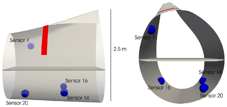
Visualization of the fatigue crack location (red face) relative to sensors 1, 14, 16, and 20.

In this work, we study the range profile relative to a baseline condition separately for every sensor and each receiving channel. In fact, the reference signal is the average of multiple baseline measurements representing a super baseline. That super baseline is subtracted from the current measurement to obtain signal differences containing the scattering response from structural changes. Differences that remain are treated as structural damage, because all other environmental variables stay constant.

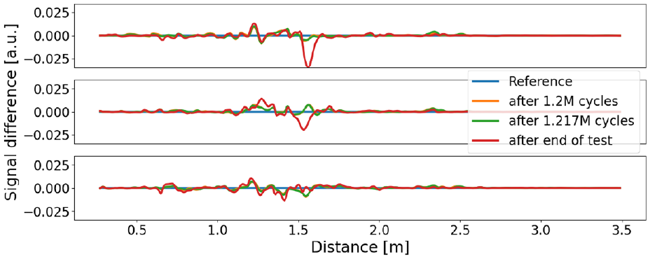
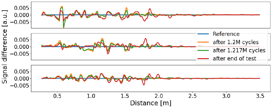
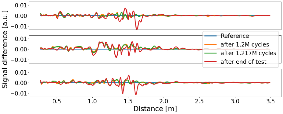
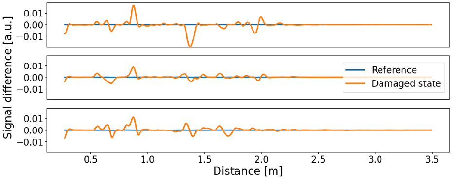
Figures 13 to 16 show differential range profiles of sensors 1, 14, 16, and 20 for all three receiving channels and for three structural states during the fatigue test, that is, reference state (intact blade), after 1.2 M cycles, after 1.217 M cycles, and after the end of the fatigue test. These time points were chosen for illustrative purposes because they were before, between, and after the last two loading phases. A range gating was performed to ignore the first 15 cm due to peaks from cross talk and interaction with the material for material-embedded sensors.

Figure 13.

Differential range profiles of channel 1 (top), channel 2 (middle), and channel 3 (bottom) of radar sensor 1.

Figure 14.

Differential range profiles of channel 1 (top), channel 2 (middle), and channel 3 (bottom) of radar sensor 14.

Figure 15.

Differential range profiles of channel 1 (top), channel 2 (middle), and channel 3 (bottom) of radar sensor 1.

Figure 16.

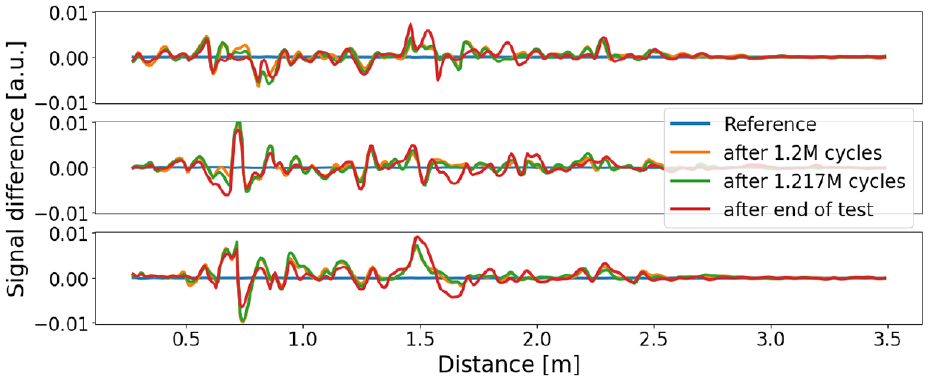
Differential range profiles of channel 1 (top), channel 2 (middle), and channel 3 (bottom) of radar sensor 20.

In all cases, the differential signals representating baseline conditions are almost zero. Significant signal changes indicate the presence of fatigue damage. This can be observed for all four sensors and all channels after the last stop and also at the end of the test. Sensor 1 shows significant signal changes at 1.5 m distance. The shortest distance from that sensor to the crack is about 20 cm. Given by a crack length of 1.5 m, the sensor probably recognizes the upper end of the crack. A similar interpretation can be done for sensors 14, 16, and 20 with significant signal changes in the range from 1.4 to 1.7 m. These distances match the distances from sensor to damage referring to the model in Figure 12.

Similar to other SHM systems, we follow a DI approach to assess the structural condition through a scalar metric. In an unsupervised approach, the DI would be monitored over time. A critical structural condition can be detected when the DI crosses a statistically defined threshold, for example, proposed by Moll and Fritzen.²⁵ The root-mean-square of the differential signal $Δ s$ is defined as

DI = \sqrt{\frac{1}{N} \sum_{i = 1}^{N} Δ s_{i}^{2}}

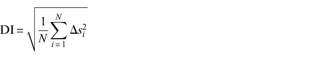
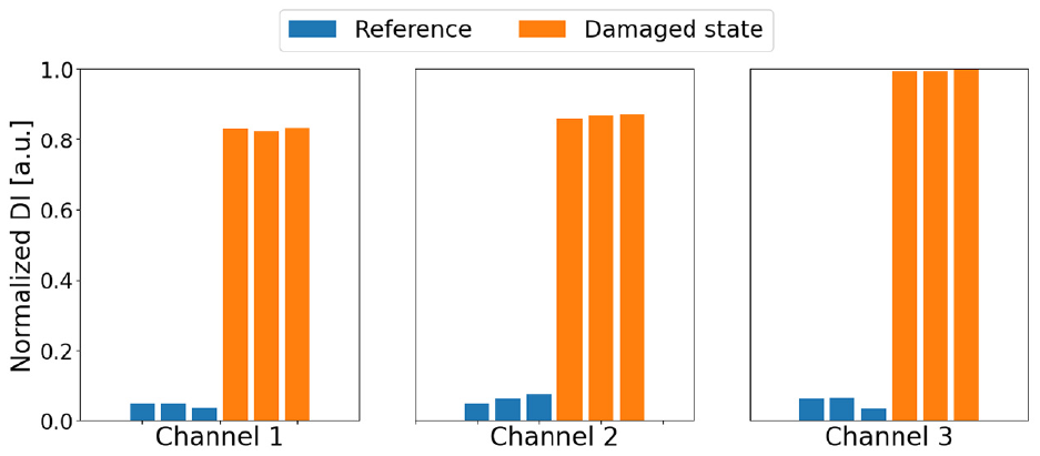
with the i-th range bin denoted as $s_{i}$ . N is the number of sample points of the differential frequency spectrum.

The DIs for sensor 1 and sensor 16 are shown as examples in Figures 17 and 18, respectively. The DIs are normalized per sensor and show small values for the intact condition and a significant increase at 1.2 M cycles and a further increase from 1.217 M cycles until the end of the test. This means that changes in the blade are detected by the radar sensors after 1.2 M cycles. This can be intermediate structural damage like delamination combined with contributions from the fatigue crack. Sensor 14 in Figure 14 shows no peaks at 1.8 m distance after 1.2 M cycles, but sensor 1 in Figure 13 and sensor 20 in Figure 16 already show peaks at 1.5 m distance after 1.2 M cycles and thus already detect fatigue damage at this point.

Figure 17.

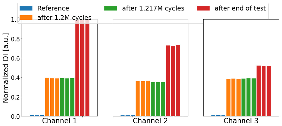
DIs for channel 1 (left), channel 2 (middle), and channel 3 (right) of sensor 1.

Figure 18.

DIs for channel 1 (left), channel 2 (middle), and channel 3 (right) of sensor 16.

Detection of artificial damages

In the previous section, a massive structural damage was studied with about 1.5 m length. However, smaller damage should be detectable with the radar sensors operating at 60 GHz. Therefore, holes were drilled into the wind turbine blade after the end of the fatigue test. Such holes are often caused by lightning strikes and are one of the common types of rotor blade damage.³ Images of the holes at the blade root and at two different positions in the web are shown in Figure 19. One of the holes in the web at z = 1.9 m is drilled completely through, where the z axis is the blade’s length as shown in Figure 2.

Figure 19.

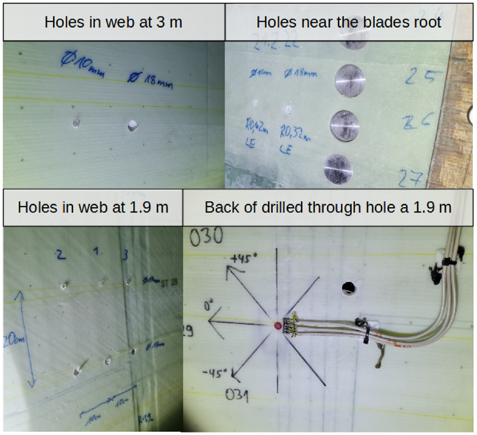
Images of drilled holes.

Figure 20 shows the differential signals for sensor 20. This sensor is within the range of all holes in the web, and it is oriented towards the web between the hole groups, thus all holes are covered by antennas sidelobes. In the differential signal, significant changes at 0.6 to 0.9 m occur which correspond to the holes at z = 1.9 m. In addition, channel 2 shows a major change for the drilled holes at z = 3 m at approximately 1.2 m distance. These distances agree with the theoretical distances from sensor to damage.

Figure 20.

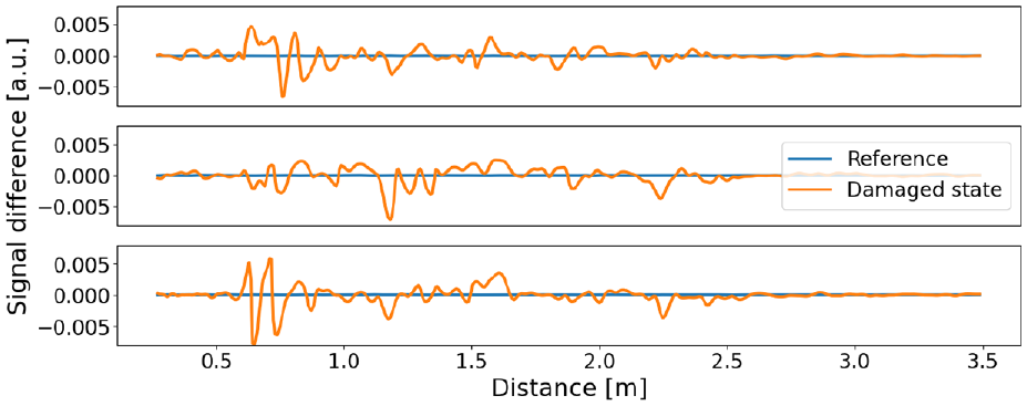
Differential range profiles after drilling holes of channel 1 (top), channel 2 (middle), and channel 3 (bottom) of sensor 20.

Figure 21 shows the differential signals for sensor 24 which faces the area of the holes near the blade root directly as well as the drilled through hole at z = 1.9 m with a sidelobe. The differential signals show indeed changes at about 0.9 m for the drilled through hole and at 1.4 m for the holes in the outer blade shell near the root.

Figure 21.

Differential range profiles after drilling holes of channel 1 (top), channel 2 (middle), and channel 3 (bottom) of sensor 24.

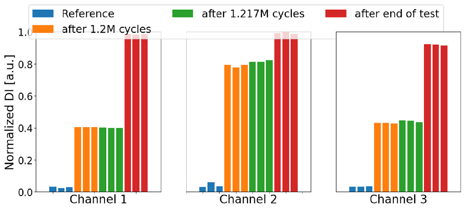
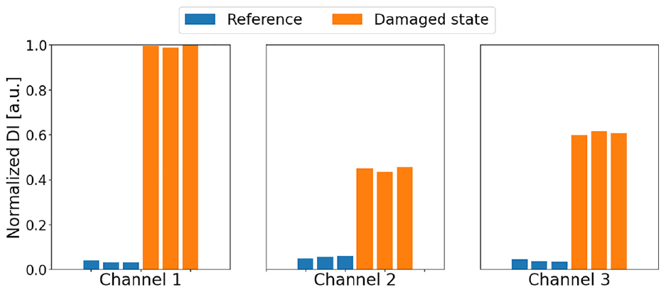
The signal changes related to the artificial damage for all channels are clearly visible in the DI representation depicted in Figures 22 and 23.

Figure 22.

DIs after drilling holes for channel 1 (left), channel 2 (middle), and channel 3 (right) of sensor 20.

Figure 23.

DIs after drilling holes for channel 1 (left), channel 2 (middle), and channel 3 (right) of sensor 24.

Conclusions

This paper described the development and realization of an embedded radar network operating at 60 GHz with sub-GHz wireless data communication that is embedded in a 31-m-long wind turbine blade during manufacturing. It was demonstrated that fatigue as well as small artificial damage in the form of holes can be detected under laboratory conditions, that is, constant environmental and operational conditions. As demonstrated in a related work by the authors, icing could be detected with such sensors as well.²⁶ This leads to the conclusion that embedded radar networks represent a promising multifaceted candidate for in situ monitoring of wind turbine blades. Also the combination of radar sensor with other sensor types in a network offers a promising approach for reliable monitoring.

The design of the radar sensor network with its integration in a wind turbine blade is already strongly oriented towards practical use in the field. However, the present study also contained several limitations that should be addressed in future research:

The measurements were carried out in a test hall under controlled conditions and the temperature fluctuated only by a few degrees. Under such conditions, the effects of environmental and operational conditions are relatively small compared to field measurements.

The energy supply of the sensors did not have to be autonomous but could be realized by cable and conventional power supply. Energy harvesting, for example, by means of solar foils, have not been implemented so far.

In the setup, four base stations for wireless data transfer have been implemented, which were positioned next to the rotor blade. Larger communication distances would be expected in the field with reduced communication performance, in particular reduced data rates.

All radar measurements evaluated in this study took place when the rotor blade was unloaded. This period is not available in the field so that mechanical vibrations as well the effects of mechanical loading must be incorporated in the data analysis. In a practical application, references for a wide range of natural deformations of the blade could be recorded in a training phase and a classification problem for damage assessment could be solved subsequently taking the changing environmental and operational conditions into account.²⁷ Monitoring of the blade’s health would thus be possible even when the rotor blade is under load.

Footnotes

Declaration of conflicting interests

The author(s) declared no potential conflicts of interest with respect to the research, authorship, and/or publication of this article.

Funding

The author(s) disclosed receipt of the following financial support for the research, authorship, and/or publication of this article: The authors gratefully acknowledge the financial support of this research by the Federal Ministry for Economic Affairs and Energy (Grant Number: 0324324C).

ORCID iDs

Jonas Simon

Jochen Moll

References

IRENA. Renewable energy statistics 2022. Abu Dhabi: The International Renewable Energy Agency, 2022.

Beganovic

Söffker

. Structural health management utilization for lifetime prognosis and advanced control strategy deployment of wind turbines: an overview and outlook concerning actual methods, tools, and obtained results. Renewable Sustainable Energy Rev 2016; 64: 68–83.

Sun

Wang

Chu

. In-situ condition monitoring of wind turbine blades: a critical and systematic review of techniques, challenges, and futures. Renewable Sustainable Energy Rev 2022; 160: 112326.

Tcherniak

Mølgaard

. Vibration-based SHM system: application to wind turbine blades. J Phys: Conf Ser 2015; 628: 012072.

Tsopelas

Papasalouros

Anastasopoulos

, et al. Acoustic emission for structural integrity assessment of wind turbine blades. Springer Proceedings in Physics, vol 158, p. 369. New York: Springer Science+Business Media.

Wen

Liu

. Wind turbine blade surface inspection based on deep learning and UAV-taken images. J Renewable Sustainable Energy 2019; 11(5): 053305.

Doroshtnasir

Worzewski

Krankenhagen

, et al. On-site inspection of potential defects in wind turbine rotor blades with thermography. Wind Energy 2015; 19(8): 1407–1422.

Rodrigues

DVQ

. A review on low-cost microwave doppler radar systems for structural health monitoring. Sensors 2021; 21(8): 2612.

Nikoubin

Muňoz-Ferreras

Gümez-Garcìa

, et al. Structural health monitoring of wind turbines using a low-cost portable k-band radar: an ab-initio field investigation. In: 2015 IEEE topical conference on wireless sensors and sensor networks (WiSNet), San Diego, CA, USA, pp. 69–71.

10.

Moll

Simon

Malzer

, et al. Radar imaging system for in-service wind turbine blades inspections: initial results from a field installation at a 2 MW wind turbine. Prog Electromagn Res 2018; 162: 51–60.

11.

Moll

Arnold

Mälzer

, et al. Radar-based structural health monitoring of wind turbine blades: the case of damage detection. Struct Health Monit 2018; 17(4): 815–822.

12.

Mitra

Gopalakrishnan

. Guided wave based structural health monitoring: a review. Smart Mater Struct 2016; 25(5): 053001.

13.

Moll

Kexel

Kathol

, et al. Guided waves for damage detection in complex composite structures: the influence of omega stringer and different reference damage size. Appl Sci 2020; 10(9): 3068.

14.

Mustapha

, et al. Sensor networks for structures health monitoring: placement, implementations, and challenges—A review. Vibration 2021; 4(3): 551–585.

15.

International Commission on Non-Ionizing Radiation Protection and others. ICNIRP statement on the “guidelines for limiting exposure to time-varying electric, magnetic, and electromagnetic fields (up to 300 GHz)”. Health Phys 2009; 97(3): 257–258.

16.

Moll

Maetz

Maelzer

, et al. Radar-based monitoring of glass fiber reinforced composites during fatigue testing. Struct Control Health Monit 2021; 28(10): e2812.

17.

Simon

Moll

Krozer

, et al. Optimized placement for embedded radar and communication sensors in wind turbine blades. In: Proceedings of the 13th International Workshop on Structural Health Monitoring (IWSHM), Stanford, CA, USA, 2022.

18.

Chmurski

Zubert

Bierzynski

, et al. Analysis of edge-optimized deep learning classifiers for radar-based gesture recognition. IEEE Access 2021; 9: 1.

19.

Kurin

Issakov

Erhardt

, et al. Analysis of a physically-embedded radar sensor system. In: 2021 18th European Radar Conference (EuRAD), London, UK, 2022.

20.

AX5043 data sheet, advanced high performance ASK and FSK narrow-band transceiver for 27–1050 MHz range.

21.

Bjørheim

Siriwardane

Pavlou

. A review of fatigue damage detection and measurement techniques. Int J Fatigue 2022; 154: 106556.

22.

Ansari

MTA

Singh

Azam

. Fatigue damage analysis of fiber-reinforced polymer composites—A review. J Reinf Plast Compos 2018; 37(9): 636–654.

23.

Shabani

Taheri-Behrooz

Samareh-Mousavi

, et al. Very high cycle and gigacycle fatigue of fiber-reinforced composites: a review on experimental approaches and fatigue damage mechanisms. Prog Materi Sci 2021; 118: 100762.

24.

Zuo

Srinivasan

Vassilopoulos

. Review of hybrid composites fatigue. Compos Struct 2021; 274: 114358.

25.

Moll

Fritzen

. Guided waves for autonomous online identification of structural defects under ambient temperature variations. J Sound Vibr 2012; 331(20): 4587–4597.

26.

Simon

Moll

Krozer

, et al. Analysis and compensation of relative humidity and ice formation effects for radar-based shm systems embedded in wind turbine blades. In: 10th European workshop on structural health monitoring. EWSHM 2022. Lecture notes in civil engineering (eds P Rizzo and A Milazzo), vol 270. Cham: Springer.

27.

Worden

Farrar

Manson

. The fundamental axioms of structural health monitoring. Proc R Soc. A: Math, Phys Eng Sci 2007; 463: 1639–1664.

Embedded radar networks for damage detection in wind turbine blades: validation in a full-scale fatigue test

Abstract

Keywords

Introduction

System description

Radar sensor description

Wireless network communication

Communication scheme

Experimental design

Rotor blade manufacturing with embedded radar networks

Description of full-scale fatigue testing

Results

Signal conditioning

Damage detection during fatigue test

Detection of artificial damages

Conclusions

Footnotes

Declaration of conflicting interests

Funding

ORCID iDs

References