
Abstract
Bridge damage detection using vibration data has been confirmed as a promising approach. Compared to the traditional method that typically needs to install sensors or systems directly on bridges, the drive-by bridge damage detection method has gained increasing attention worldwide since it just needs one or a few sensors instrumented on the passing vehicle. Bridge frequencies extracted from the vehicle’s vibrations can be good references for damage detection. However, extant literature considered mainly low-frequency responses of the vehicle, while the high-frequency responses that also contained the bridge’s damage information were often ignored. To fill this gap, this paper developed a damage detection approach that utilized both low and high-frequency responses of the passing vehicle. Mel-frequency cepstral coefficients (MFCCs) and support vector machine (SVM) were employed to classify damage severity. Firstly, the vehicle’s frequency responses are utilized as input features to train SVM models to identify the bridge’s condition. Then, to reduce dimensions of inputs and improve training efficiency, frequency responses are projected from the Hertz scale into the Mel scale, and two means using MFCCs are used to feed different SVM models. A laboratory experiment with a U-shaped continuous beam and a model car was used to verify the effectiveness of the proposed method. Results showed that high-frequency responses contain much information about the bridge’s conditions, and using MFCCs could apparently improve computational efficiency. The errors of damage detection when a heavy car was employed were within 5%.
Keywords
Introduction
Bridges are essential components connecting transport networks all over the world. Aging, deterioration, and failure of bridges can pose threats to human lives. According to the infrastructure report in the U.S. in 2021, around 42% of bridges in the U.S. are over 50 years old. 1 Structural health monitoring (SHM) is increasingly essential since it can provide the bridge’s safety assessment and predict its remaining life. 2 As a principal branch of SHM, damage detection has gained much attention in the last decades. Traditionally, damage detection is on the basis of visual inspection by qualified engineers. 3 However, with the fact that bridges’ span, complexity, and height are greatly increasing, visual monitoring becomes time-consuming, dangerous, and even unachievable. Using vibration data of bridges is confirmed as a promising way to solve this problem.4–6 The bridge’s dynamic characteristics before and after damage are good references for damage detection.
Conventionally, sensors are attached directly to the bridge to collect its vibration data to extract the bridge’s dynamic properties. A monitoring system may be installed and maintained for the bridge in the long run, 7 and typically, one system can perform well for one unique bridge. Even though the direct method can accurately record the bridge’s vibration data and perform analysis in real time, it is challenged by high deployment costs, hostile field environment, battery capability, etc. Besides, after sea-like data are obtained, most of them are saved and cannot be effectively used. Due to the above reasons, only gigantic and crucial bridges are equipped with these monitoring systems. However, a large part of bridges worldwide are short and mid-span bridges, which are not appropriately monitored.
To solve this problem, the drive-by damage detection method was proposed. This method was firstly proposed by Yang et al. 8 in 2004, and the authors successfully extracted the bridge’s fundamental frequency using the passing vehicle’s vibration data. Later, the proposed method was confirmed by Lin and Yang 9 in a field test. A salient advantage of this method is that it just needs one or a few sensors installed on the passing vehicle; thus, it is economical and easy-to-operate. Besides, the vehicle itself can play the exciter and sensor roles, so no particular excitation is needed. The potential of the drive-by method ensured that the passing vehicle’s vibration data contained the bridge’s critical dynamic characteristics and could be used as references to monitor its health conditions.
As one of the essential properties of bridge structures, the frequency was commonly researched using the drive-by vehicle’s vibration data. Many scholars have been contributing to extracting bridge’s natural frequencies to estimate the bridge’s states. To increase the precision of frequency extraction, Yang and Chang 10 found that by decreasing the amplitude ratios between the vehicle and bridge’s acceleration amplitudes, the probability of successfully extracting the bridge’s frequencies from the vehicle’s vibration data could be increased. The first two natural frequencies of the bridge were successfully obtained. To extract high modes, empirical mode decomposition was used to preprocess the vehicle’s time-domain accelerations into intrinsic mode functions (IMFs). It was found that using IMFs could significantly improve the visibility of the bridge’s frequency.11–13 On the other hand, it is worth noting that the frequency of the bridge is a comprehensive dynamic parameter; thus the extracted natural frequencies may not be sensitive indicators for damage detection. Local damage may not be able to induce a significant change in the bridge’s natural frequencies. 14 Therefore, frequencies may not be ideal indicators for bridge damage detection. As a result, researchers began to focus on the Frequency Response Function curve of the passing vehicle rather than just peaks in the frequency spectrum. Cerda et al. 15 tried to detect changes in the bridge using the vehicle’s frequency responses. Four different masses were added to the bridge, and five different car speeds were used. Employing Short Time Fourier Transform (STFT), the acceleration was transformed from time domain to frequency domain. Then, correlation coefficients between averaged health and damaged spectrum were used to identify the damage. Compared to the direct method with sensors installed on the bridge, the indirect monitoring results could reach an acceptable level. However, the vehicle’s frequency responses generally contain many components that may cover changes induced by the bridge’s health conditions. One of them is the influence of road roughness. Different passing road roughness can induce changes in the vehicle’s frequency spectrum. To this end, Nagayama et al. 16 utilized two connected passing vehicles to eliminate the effect of road roughness. Both numerical simulations of a 59 m long box-girder bridge and field tests showed that the bridge’s frequency could be identified accurately, and the influence of road roughness could be removed. Wang et al. 17 proposed to utilize the vehicle’s front and rear axles responses to eliminate the influence of roughness, so the input in the vehicle’s responses just contained the bridge’s vibration. Therefore, the bridge’s frequency-domain responses could be obtained clearly. Another influence comes from the vehicle itself. Since sensors are installed on the vehicle, its frequency would predominate in the frequency domain. If the vehicle’s frequency can be invisible in frequency responses, it would be easier to identify the bridge’s conditions according to its frequency domain responses. Yang et al. 18 suggested that a filter could be used to eliminate the vehicle’s frequency in its frequency spectrum. Two numerical examples verified the effectiveness of the proposed filtering method. Later, Yang et al. 19 proposed using contact-point (CP) response rather than the vehicle’s vibration data. The CP responses can outperform the vehicle’s response because the vehicle’s frequency will disappear in the frequency spectrum, but the bridge’s frequency responses remain. Bridge frequency response extraction using the CP response was proved robust under the influence of existing traffic and road roughness. However, in existing literature, only low-frequency responses are concerned because high-frequency responses are easily contaminated by noises. On the other hand, as sensors are installed on the passing vehicle, most high-frequency responses are related to the vehicle’s properties rather than the bridge. These two reasons make the exploration of high-frequency responses difficult. Still, high-frequency responses of the passing vehicle contain the bridge’s damage information as well and thus have the potential for damage detection.
Due to the rapid development of computer hardware, machine learning (ML) techniques have been gradually employed in the last decade. It has been utilized in frame and truss structures, 20 turbine damage detection, 21 direct bridge monitoring, 22 dam safety monitoring, 23 etc. In recent years, researchers started to use ML in drive-by bridge damage detection. Liu et al. 24 proposed that full-bandwidth frequency responses should be utilized because high-frequency responses can contain the bridge’s damage information. The authors employed stacked autoencoders to achieve dimension reduction, then a semi-supervised model was trained to identify damage in bridges. The test results showed that damage detection precision could reach 15 g (different masses were added to the bridge to simulate damages). Malekjafarian et al. 25 utilized an artificial neural network (ANN) to project frequencies and the vehicle’s speed into its frequency responses. An ANN model was trained using healthy cases, and then the same model was used for damage cases. The damage severity was indicated by comparing the difference between predicted and true frequency responses. Sarwar and Cantero 26 considered several vehicles passing the bridge at the same time, and a deep autoencoder (DAE) model was set up for training. When the bridge was healthy, thousands of passing vehicles’ vibration data were used to train the DAE model. Then, the trained DAE was used to encode and decode vibration data of unknown cases. The mean absolute error between the vehicle’s vibration and predicted data was utilized as damage indicators. The numerical simulation showed that the DAE could accurately identify the bridge’s damage. Locke et al. 27 proposed to consider the environmental effects on drive-by health monitoring. The vehicle’s frequency-domain responses were used to train modified VGG19 28 neural networks (NN). Considering vehicle traffics, surface roughness, and temperature, the numerical examples showed that the NN model could learn the bridge’s damaged state from the passing vehicle’s vibration data and, to some degree, eliminate environmental noises. Corbally and Malekjafarian 29 proposed to utilize frequency-domain CP responses as the ANN’s input, and the influence of temperature was considered in long-term monitoring progress. An ANN model was trained to identify the impact of temperature and detect bridge damage. Results showed that using the CP responses outperformed traditional accelerations of the passing vehicle and was robust under the influence of different vehicle speeds and road roughness. However, in the previous work, the calculation process, either very complex or with no high-frequency responses, was utilized, making the damage detection process challenging to apply in practical engineering.
In this paper, an approach to identify bridge damage utilizing the passing vehicle’s low- and high-frequency responses is proposed. Different vehicle speeds (between 0.7 and 1.1 m/s) and weights (normal and heavy) are considered. The idea is explored using a steel bridge and a model car in the lab. Two sensors are installed on the front and rear axles of the vehicle to collect its vibration data. Then, the vehicle’s frequency-domain responses are used to train an support vector machine (SVM) model to classify whether the bridge is damaged or not. To improve the damage detection efficiency and precision, Hertz scale frequencies are transformed into Mel scale, and then Mel-frequency cepstral coefficients (MFCCs) are extracted as input features. MFCCs are originally from acoustic recognition, and they are used to extract features of sounds. Recently, it has been found that MFCCs can be used in SHM, and good results have been obtained on pipeline anomaly detection, 30 bridge decks monitoring, 31 and bolt looseness detection, 32 etc. However, the combination of MFCCs and ML techniques are rarely used in indirect bridge health monitoring to the author’s best understanding. The remainder of this paper is organized as follows: Section “MFCCs and SVM based methodology” introduces the principles and process of applying MFCCs and SVM to drive-by damage detection. Section “Lab-scale experiments” explains the setup for the laboratory experiments. Section “Experimental results and discussions” discusses the hyperparameter selection of calculating MFCCs and building SVM models and discusses the results of bridge damage detection. Section “Conclusions and future work” provides conclusions and future work for this paper.
MFCCs and SVM-based methodology
Mel-frequency cepstral coefficients
MFCC is a particular cepstrum that has been proved as an effective method in acoustic feature identification. It is designed to present the results of a cosine transform of the real logarithm of the short-term energy spectrum on a Mel-frequency scale. MFCCs are expected to focus on a range of frequency responses, compared to Hertz-frequency in which only high amplitudes will be considered. Owing to this, MFCCs can be used to reduce the dimensions of frequency-domain responses. Besides, different from traditional cepstrum that treats frequency range the same, MFCCs focus more on low frequencies but do not ignore high frequencies completely, so they still can consider all frequencies. Originally, MFCCs are designed to simulate how people can hear sounds (human beings’ auditory system is linear under 1 kHz but logarithmic over 1 kHz). 33 MFCCs utilize these characteristics to analyze signals when processing sounds and can successfully extract features of the input acoustic signals. The original mutual transitions between Hertz and Mel frequency scale are presented in Equation (1).
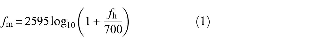
where
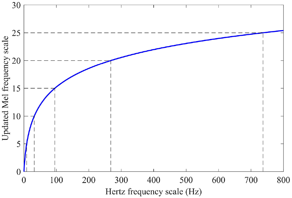
Relationship between Hertz and Mel frequency scale (0–800 Hz).
In the process of extracting MFCCs from acceleration signals of the passing vehicle, five steps are involved: (1) Data preprocessing; (2) Fast Fourier Transform (FFT); (3) Mel Filter bank; (4) Logarithm; (5) Discrete Cosine Transform (DCT). The order of data processing is shown in Figure 2, which is introduced below.
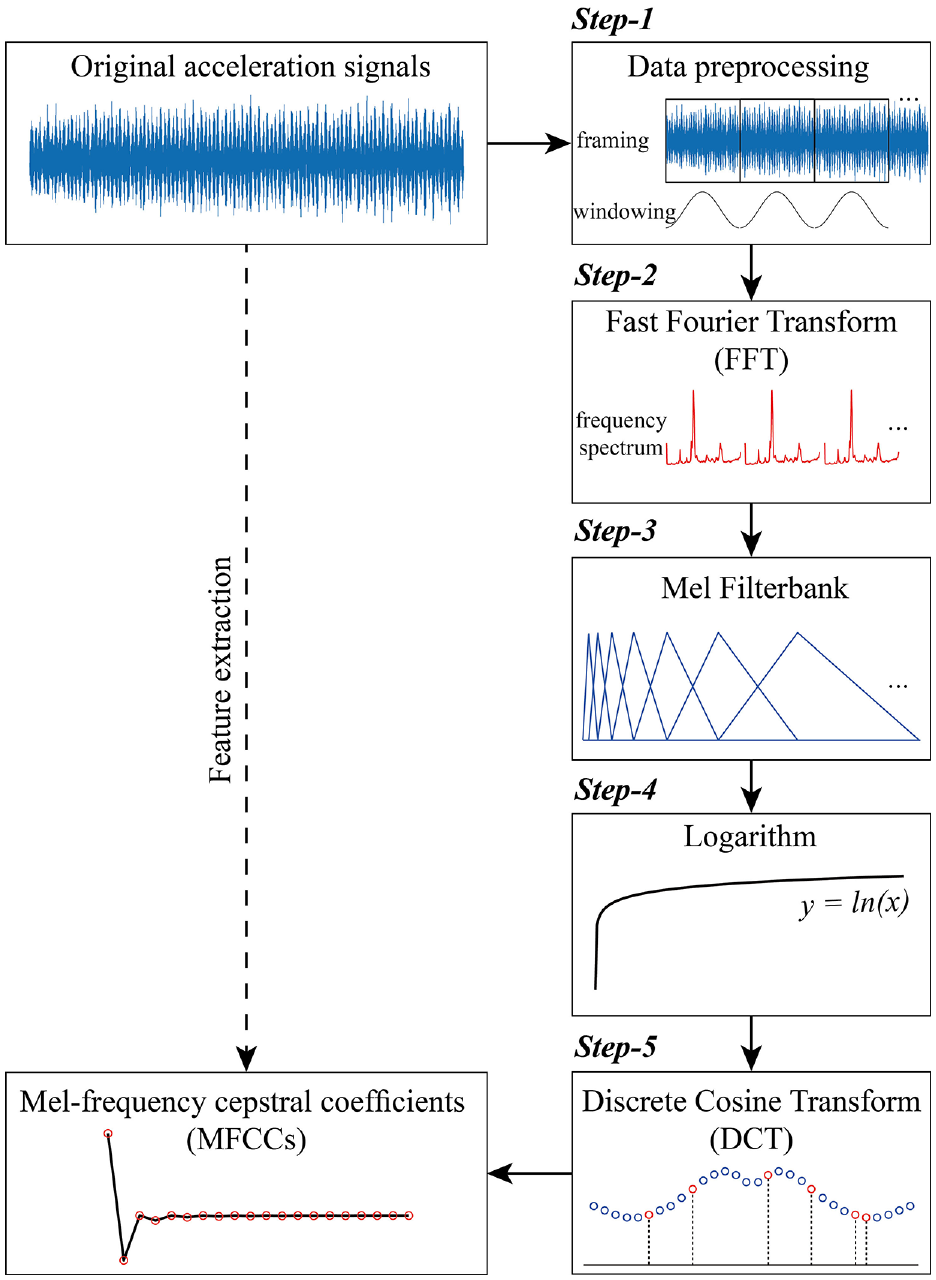
Five steps to extract MFCCs from original acceleration signals.
Data preprocessing
Before transforming the vehicle’s acceleration signals into the frequency domain, they need to be preprocessed. Since the vehicle’s front axle will firstly be driven to the bridge and then the rear axle (there may be multiple axles), the time when the front tires enter the bridge is set as

Then acceleration signals within
Because the signal is divided into different frames directly, spectrum leakage may occur due to signal truncation. A promising way to solve this problem is to add windows to divided signals. General windows include rectangular window, Hann window, Hamming window, Flat top window, etc. Since the amplitudes of the passing vehicle’s vibration signal do not vary very much, the Hann window is selected in this paper.
Fast Fourier transform
Fast Fourier transform (FFT) is quite commonly used in signal processing for SHM. It can transform signals from the time domain to frequency domain for further analysis, but it cannot represent time sequence information for signals. The STFT can be utilized to solve this problem. That is to divide the signal into several sections in time sequences, and for each sequence, FFT is performed. Since the acceleration signals are divided into several frames, STFT is adopted in this paper. Furthermore, the energy of signals can be obtained from their frequency-domain responses. A general way to calculate the energy spectrum is to calculate the square of frequency-domain responses, which is employed in this paper.
Mel Filter bank, logarithm, and discrete Cosine transform
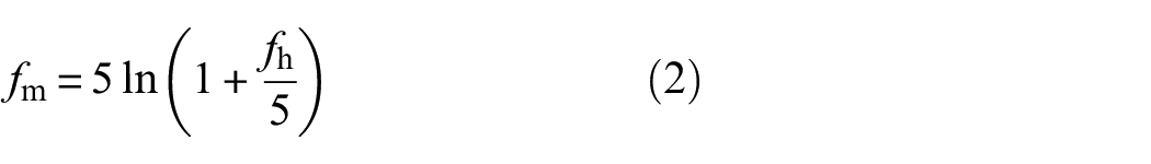
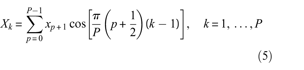
For each energy spectrum, Equation (2) is used to project it into the Mel frequency scale. In the Mel frequency scale, linear frequency ranges (increasing in the Hertz frequency scale) are selected. Then the energy spectrum in the Hertz scale is convolved with Mel filter banks. For example, if 0–800 Hz in Hertz scale is divided into 15 filter banks evenly or unevenly in Mel scale using Equation (2), the results can be found in Appendix. After that, a logarithm and a Discrete Cosine Transform (DCT) are applied for each bank to obtain the final MFCCs.
The above five steps can be represented in Equation (4)
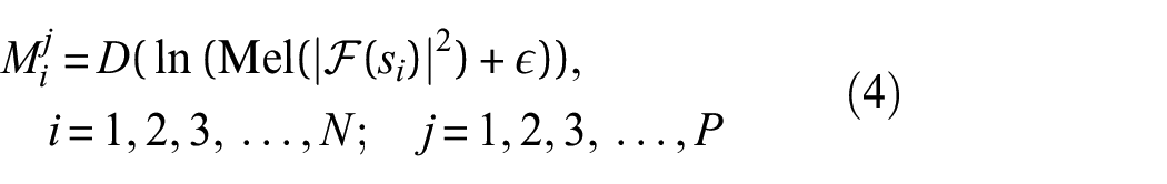
where
In acoustic recognition, the first MFCC is usually dropped because it is very sensitive to the amplitudes of signals. However, in the ML process, the machine can automatically learn whether the first coefficient will play a role or not. Therefore, all MFCCs are selected in the later sections for bridge damage detection.
Support vector machine
SVM is a vital algorithm in ML and has interested many researchers in SHM36–38 owing to its good performance in classification problems and its explainable characteristics. SVM has been successfully employed to traditionally direct SHM, but few studies have been done to detect bridge damage using drive-by vibration data. The principles of SVM employed in indirect bridge damage detection will be introduced in this section.
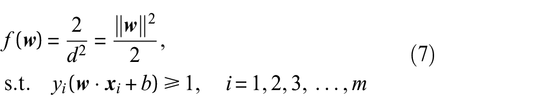
The basic idea of SVM is to maximize the margin between two classes using a hyperplane shown in Figure 3. If the datasets own m samples presented by

where
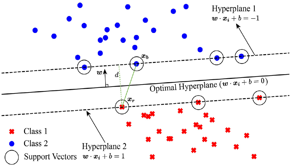
Basic principles of SVM.
To seek for the minimum of Equation (7), its dual problem is considered. A confirmed method to solve this optimization problem is called the standard Lagrange multiplier method as introduced in Equation (8), which includes two parts: the original problem and the inequation constraint. By introducing the Lagrange dual function (Equation (9)) that only consists of
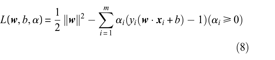
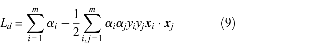


where
When the data cannot be separated perfectly by a linear hyperplane, the margin needs to be adjusted. Thus,
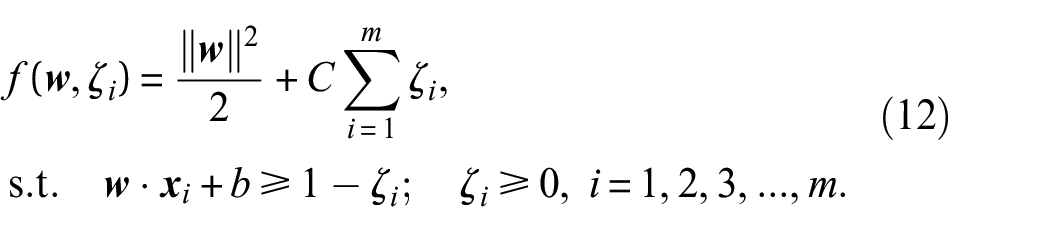
where C is used to control how much the objective function needs to be penalized. When C is huge, SVM does not allow errors in classification problems so that the margin will be smaller (hard margin); instead, if C is small, some classification errors can be acceptable and the margin can be bigger (soft margin).
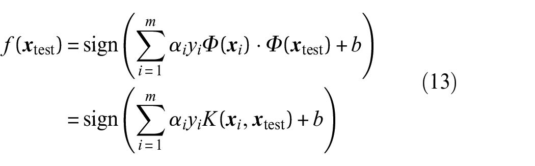
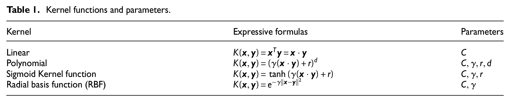
For nonlinear classification problems, data need to be mapped from the original space
Kernel functions and parameters.
Damage detection
This section will discuss the bridge’s damage detection using the proposed method. The proposed idea in this paper is a baseline-based method, which requires that the bridge is healthy at the beginning when the passing vehicle’s vibrations are recorded. At this stage, a large number of runs (named “healthy” runs) are needed to suppress the random influence of different factors, such as environmental noises. Then, new runs (named “unknown” runs) will be collected regularly by the vehicle to check the bridge’s healthy state. Then, the same number of runs from “healthy” and “unknown” runs will be utilized to train the SVM model. If the SVM model employing MFCCs can classify the “healthy” and “unknown” runs with high accuracy, the bridge is regarded as damaged. However, if the SVM cannot be trained well and the accuracy is very low (nearly 0.5), we will understand that the bridge maintains its healthy state.
Lab-scale experiments
Experimental setup
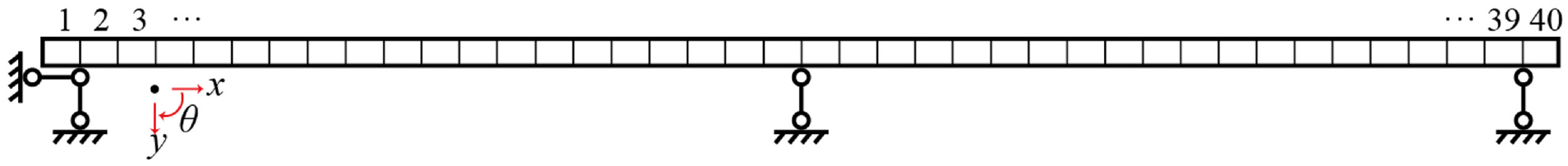
In this section, lab experiments are performed to verify the proposed idea. A continuous UPE300 beam made of Q355 steel is utilized in the experiment. The beam’s flange thickness is 15 mm, and the web thickness is 9.5 mm. Its width is 100 mm and the height is 300 mm (shown in Figure 4(a)). The beam is rotated anticlockwise at 90° to simulate the field bridge. The total length of the bridge is 6.0 m. There are two spans, and each one is 2.85 m. The support length is 0.15 m at each end (see Figure 4(a)). The total mass of the bridge is 248.64 kg. A Tamiya model car driven by a remote-control unit (see Figure 4(b) and (c)) is utilized to simulate the real car on bridges. Besides, two guide cables are utilized to drive the car straightaway. Note that guide cables will not constrain the car’s vertical vibration, and because the cables are not very tight, the car’s passing tracks on the bridge are different. The car has its suspension system, connection shaft, rubber tires, etc. Its self-weight is 4.305 kg (normal car). The front axle’s weight is 2.102 kg, and the rear one is 2.203 kg. In the experiment, 5.157 kg of extra mass is also added to the car so that its weight becomes 9.462 kg (heavy car), with the front axle’s weight of 4.315 kg and the rear axle’s weight of 5.147 kg. In the later analysis, the heavy car is selected for analysis at first. Two accelerometers, type 4371 made by Brüel and Kjær, are installed on the car’s front and rear axles (see Figure 5(a)) to collect acceleration data. Several accelerometers are also attached to the bridge’s bottom to compare with the traditional direct bridge damage detection method (see Figure 5(b)). Because this paper aims to also analyze high-frequency responses, the sampling frequency is set as 10 kHz. Other devices include: a laptop to save data, the I/O device, and signal amplifier sets. The experiment is performed in the structural laboratory at Aalto University with normal environmental noises.
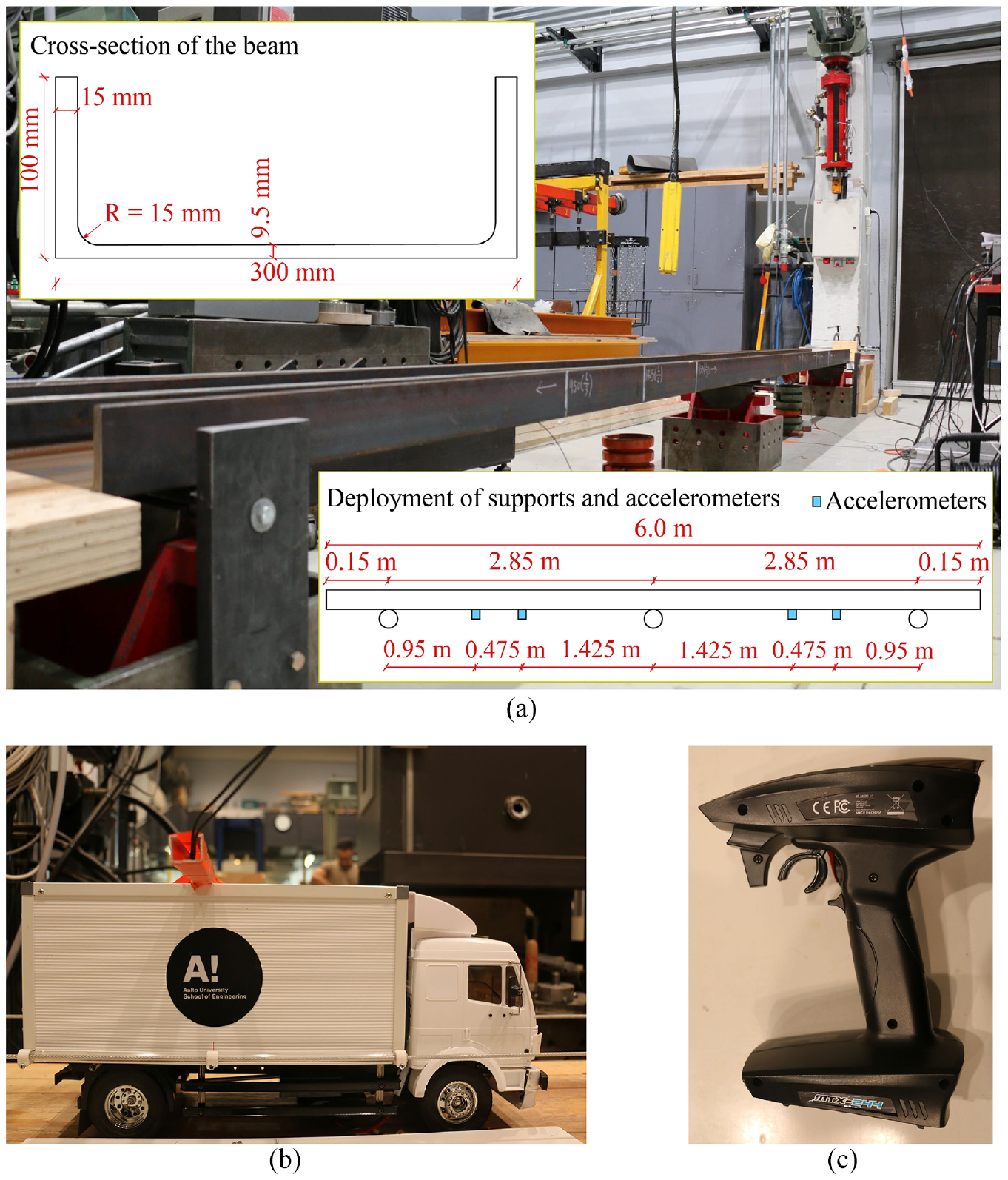
Experimental setup: (a) continuous beam, (b) model car, and (c) remote-control unit.
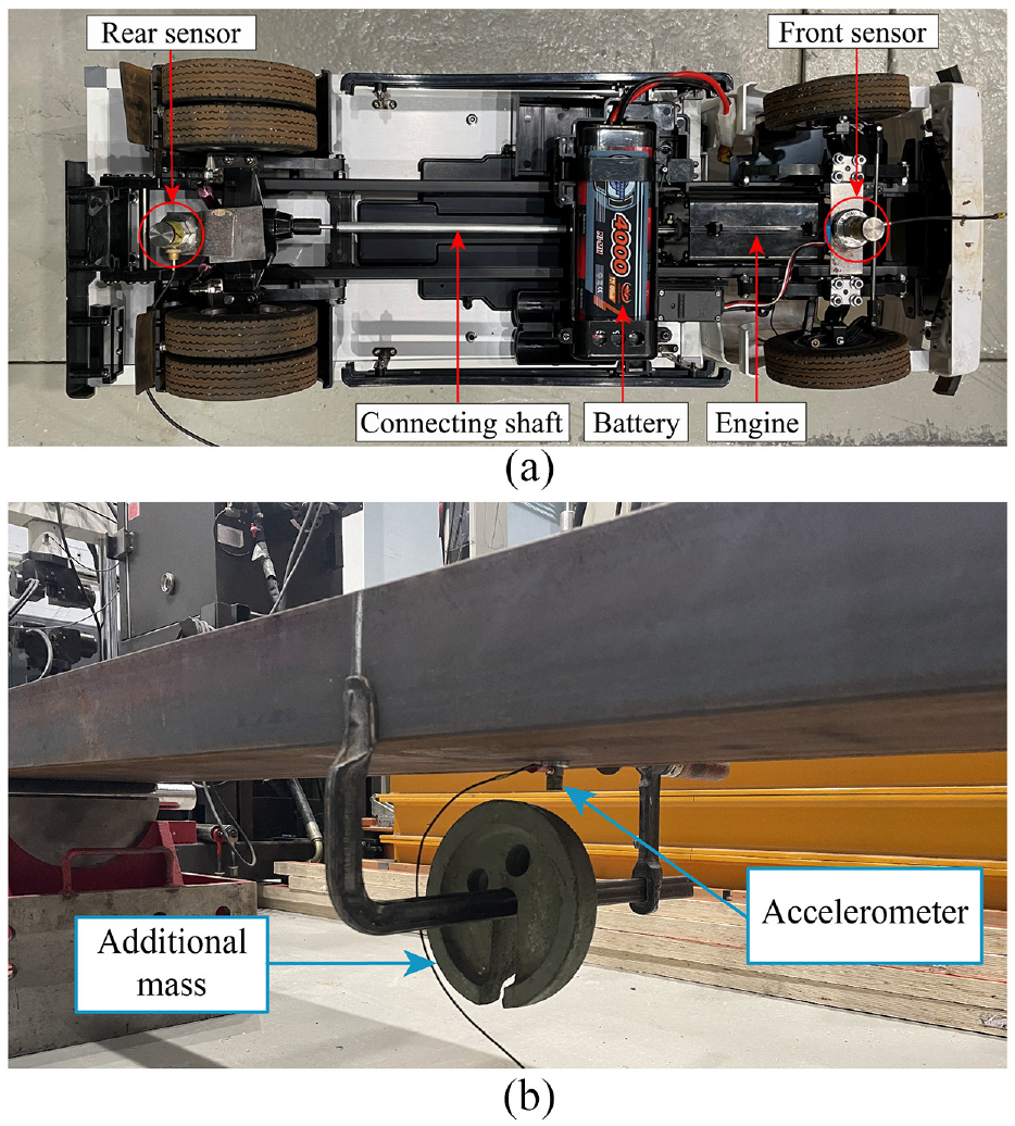
Accelerometers and additional mass: (a) sensors installed on the car and (b) additional mass to the bridge (5 kg).
The car is driven using the remote-control unit. Before the vehicle enters the bridge, there is an acceleration zone where the vehicle can accelerate from a static state to the highest speed. Similarly, the deceleration zone is set at the end of the bridge, so the car can decelerate after passing the bridge. Both the acceleration and deceleration zones are made of wood. As mentioned before, acceleration data are utilized for analysis only when both the front and rear wheels are on the bridge. In this way, all data are collected when the car is at its highest speed. However, as the capability of different batteries is different and a battery’s performance decreases if it is used for a long time, the highest speeds of various passages are different. It is to simulate that in practical engineering, a car’s passing speeds are different as well. In this experiment, there are 796 heavy car runs in total. The speed’s histogram and cumulative distribution are shown in Figure 6. It can be seen that the car’s speed is approximately subject to Normal distribution. Fitting a Normal distribution, car speed’s fitted probability density function, and cumulative distribution function are shown in Figure 6. The mean value and variance are 0.908 m/s and 0.048, respectively.
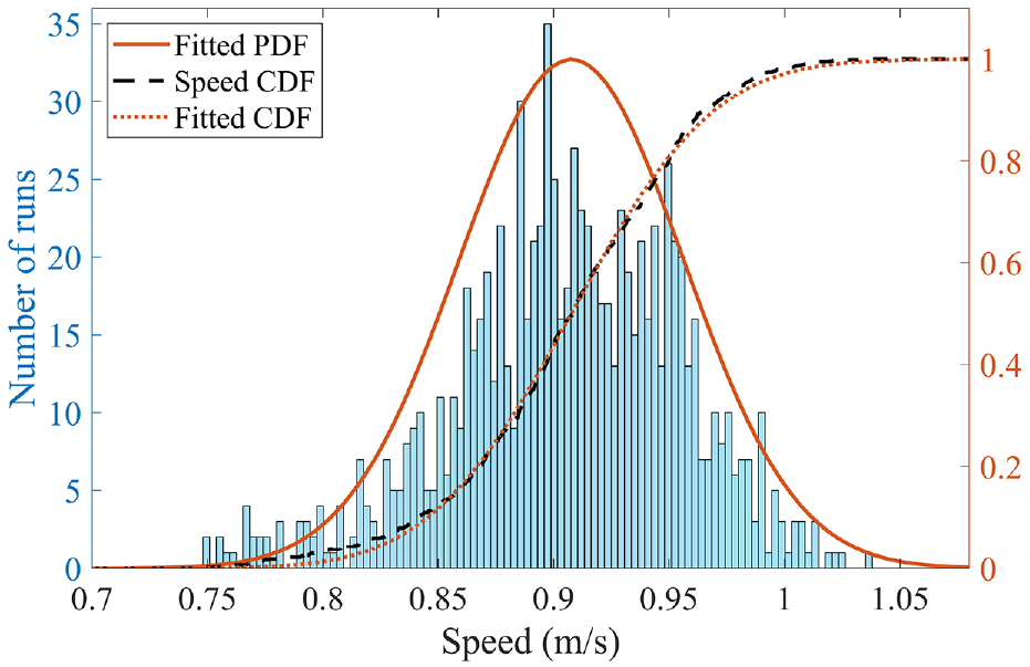
Car’s speed distribution.
Bridge’s damage
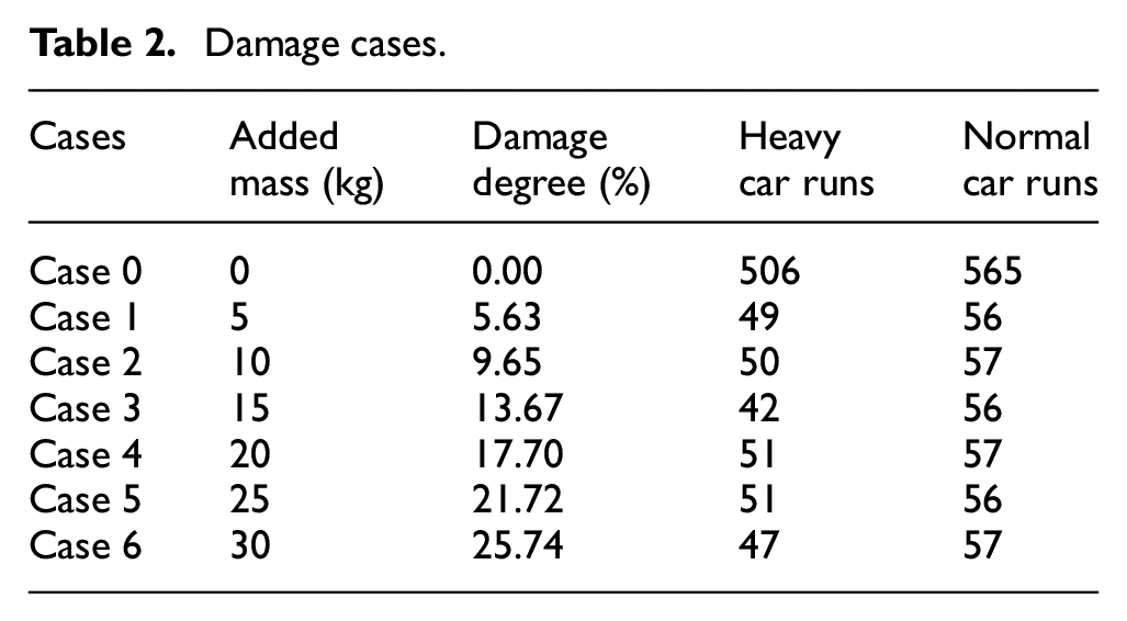
The bridge’s damage can typically induce the deduction of its stiffness. In the frequency domain, it was found that real damages can induce changes in the bridge’s frequency responses. 39 Similar effects can be made by adding masses to the structure. The effectiveness of this method has been verified by several studies, such as references.24,40–42 In this experiment, different additional masses are employed to simulate different damage cases. The mass is added to the middle of each span. There are seven cases in total: 0 (intact), 5, 10, 15, 20, 25, 30 kg. For example, the case of adding 5 kg to the bridge can be seen in Figure 5(b). The beam with no extra mass is considered intact. Two hooks are used to add the mass to the bridge, and each hook’s mass is 2.0 kg. The damage degree is represented by the percent of added masses out of the bridge’s mass. All seven cases are summarized in Table 2.
Damage cases.
Data training and testing
In this paper, scikit-learn package 43 is utilized to perform classification using SVM. Two different features, including frequency responses and MFCCs, are used. The performances of using raw frequency responses and MFCCs with even or uneven bank filters are compared. The features with better performance are selected for further analysis. For each training and testing, a 5-folder cross-validation (CV) strategy is used to avoid the occasionality of grouping data. That means 4/5 of the samples are used for training, and the rest of the samples are used for testing. This process will be done five times. Then, the mean test accuracy is recorded for analysis. When the SVM is utilized for the binary classification problem, the same number of runs from the intact case (case 0) and damaged cases (cases 1–6) will be selected for training and testing. Take case 1 as an example. Since there are 49 runs of it, 49 samples are randomly selected from 506 samples of case 0. In this circumstance, if the testing accuracy is around 0.5, it means that the SVM cannot classify these two classes because even though the SVM labels all samples as intact or damaged, the accuracy can still reach 0.5. The above random selection process will be performed 10 times for each training and testing. For the multiclass classification problem, 50 runs are randomly selected from all 506 runs in case 0. Other sample selection processes will be the same as binary classification.
Experimental results and discussions
Low frequency response analysis
In the experiment, vibrations of both the car’s front and rear axles are recorded. But because they do not have an apparent difference, only the rear axle’s vibration is utilized in the following analysis. Two examples of time-domain vibration data in case 0 and case 1 are shown in Figure 7(a).
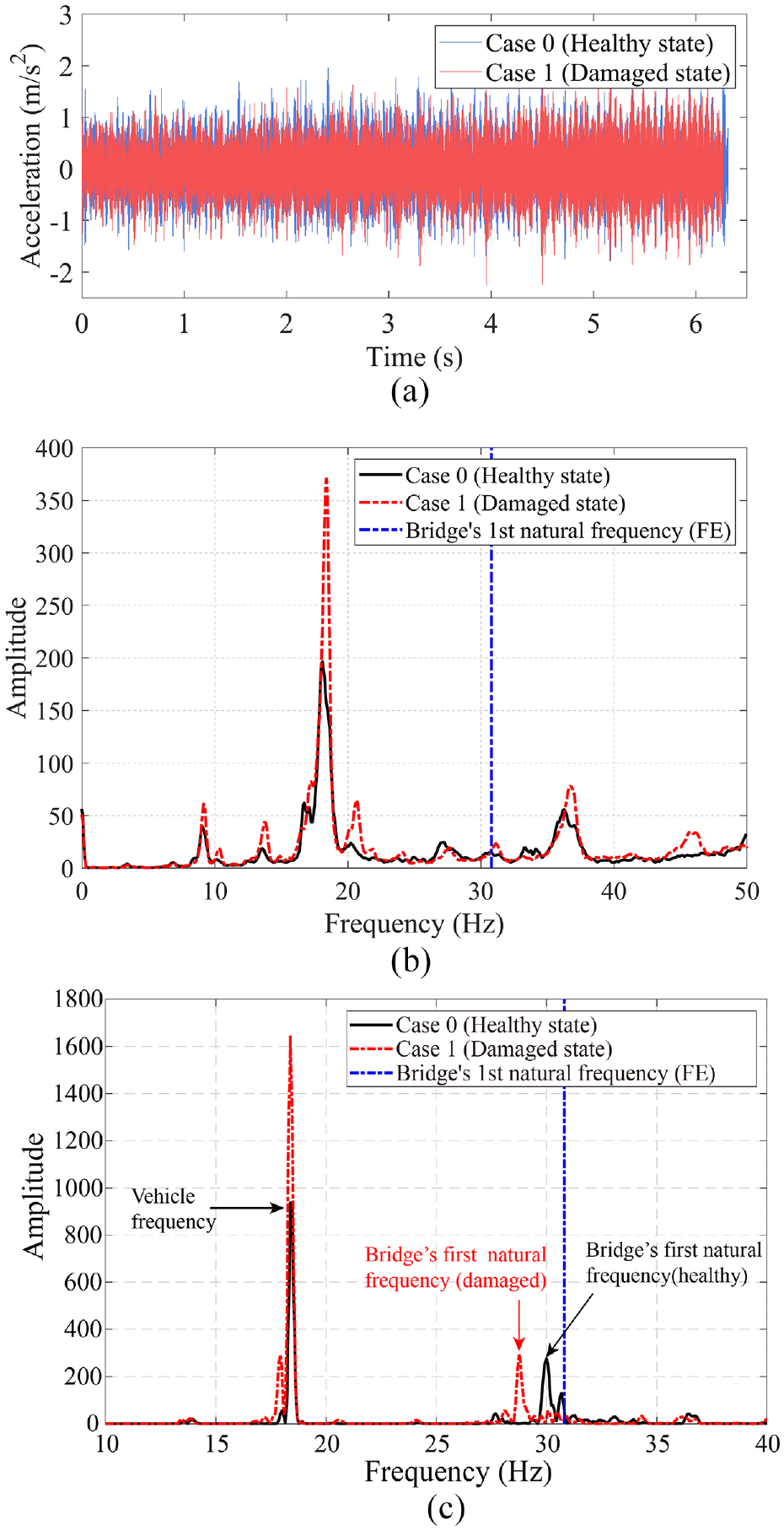
Responses of indirect and direct methods: (a) time-domain responses of intact and damaged cases, (b) frequency-domain responses for intact and damaged cases, and (c) Bridge’s frequency responses (direct method).
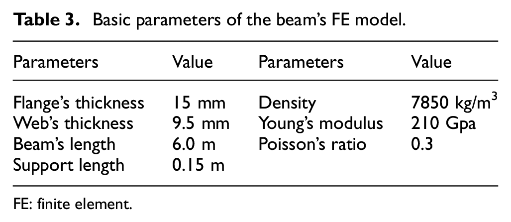
It can be seen from Figure 7(a) that the time-domain signals are nearly the same in both intact and damaged scenarios. Therefore, it is necessary to find suitable features to determine whether the bridge is damaged or not. Since the vibration data of passing vehicles contain the bridge’s dynamic properties, the analysis of the frequency-domain responses may provide important information about the bridge’s damage. Employing FFT, the time-domain signals are transformed into the frequency domain. For frequency-domain analysis, the averaged frequency responses of case 0 and case 1 are used so as to eliminate the influence of noise as much as possible. As high-frequency responses typically include noisy frequencies and cannot be recognized by eyes, only 0–50 Hz frequency responses are shown in Figure 7(b). To analyze the beam’s natural frequency in the vehicle’s frequency domain, the two-span continuous beam’s finite element (FE) model is built using beam element in MATLAB as shown in Figure 8. The basic parameters of the FE model can be found in Table 3. The FE model has 40 elements and 41 nodes, and each node has three degrees of freedom: x-translation, y-translation and rotation
FE model of the continuous beam.
Basic parameters of the beam’s FE model.
FE: finite element.
It can be seen from Figure 7(b) that for case 0, the bridge’s first-order natural frequency can be identified if it is known beforehand, but the amplitude around 30.809 Hz is pretty weak. Because of the existence of environmental noises, engine noises, and the vehicle’s dynamic parameters, it is hard to extract the bridge’s first-order frequency directly. It can be seen that the vehicle’s frequency-domain responses of passing intact and damaged bridges do not have much difference. In addition, the two cases’ highest amplitudes are different as well, so it is unknown whether the highest amplitudes are the vehicle’s frequency or the bridge’s first order frequency. Therefore, it is difficult to determine whether the bridge is damaged or not from the car’s frequency-domain responses directly.
For comparison, data of the traditional direct method (sensors on the bridge) are plotted as shown in Figure 7(c). The difference between the measured and the simulation results can be caused by the assumptions of various data such as damping ratio, material density, Young’s modulus, etc. Frequency-domain analysis of the bridge’s vibration shows that its first-order natural frequency decreases because of the additional mass, but the vehicle’s frequency remains the same no matter if the mass is added or not. This change cannot be identified from the vehicle’s frequency response. Other methods are expected to be used to find the difference between intact and damaged cases using the passing vehicle’s vibration.
SVM using frequency responses
As aforementioned, it is generally hard to determine the health condition of the bridge by using only low-frequency responses. This section utilizes both low- and high-frequency responses to determine the bridge’s state. Since the frequency spectrum is symmetrical, half of the spectrum is selected for analysis. In this experiment, it means 0–5000 Hz, and the frequency resolution is 0.0763 Hz. There are 65,537 frequency response points in total, and all these points are utilized as features to train SVM models. Initially, for SVM models, all hyperparameters are set as constant values:
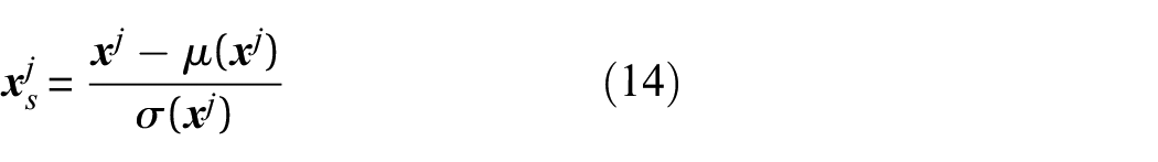
Before training the SVM model, a common way to improve the accuracy is to normalize all features. The Kernel calculation, especially linear and Polynomial Kernel, will be quite slow when all features have their units. Occasionally, Radial basis function (RBF) and Sigmoid Kernel may not be able to address non-normalized data. Normalizing all features can greatly improve computational efficiency. General normalization methods include StandardScaler and MinMaxScaler. StandardScaler can make all feature data normally distributed, and it can be calculated by Equation (14), where
By employing StandardScaler and inputting frequency responses of samples in a specific range into SVM models, we can get an accuracy using the responses in the selected frequency range for testing samples (introduced in Section “Data training and testing”). When the responses in different frequency ranges are utilized, different accuracy will be obtained accordingly.
Figure 9(a) plots the change of accuracies when the selected range increases from 0–0.0763 to 0–1500 Hz. It can be seen that with the increase in the selected frequency range, the test accuracy of Linear and Sigmoid Kernel is increasing. Rather, when Polynomial and RBF Kernels are employed, the test accuracy is poor. The main reason for this phenomenon is the high sensitivity property of the latter two Kernels to their hyperparameters. Those hyperparameters must be systematically modified to improve their performance. Further Kernel selection will be discussed in Section “Selection of filter banks’ number and SVM Kernel.” For the Linear Kernel, we can see that when the selected frequency range increases to 0–300 Hz, the test accuracy is much better than the scenario when only frequency responses in 0–60 Hz are employed. When the growth of the utilized frequency range continues further to 0–750 Hz, the test accuracy tends to be stable (accuracies when the frequency range increases beyond 0–1500 Hz are not plotted because they have been relatively stable). Therefore, high-frequency responses of the vehicle can also contribute to damage detection for the bridge. In practical engineering, compared with the beam employed in this experiment, a real bridge’s natural frequencies are typically smaller. 17 Thus, the frequency range of 0–750 Hz used in the experiment will also be applicable for a real bridge. However, the natural frequencies of different bridges can vary significantly. To ensure good results, the authors recommend selecting 0–1000 Hz frequency responses for a practical application.
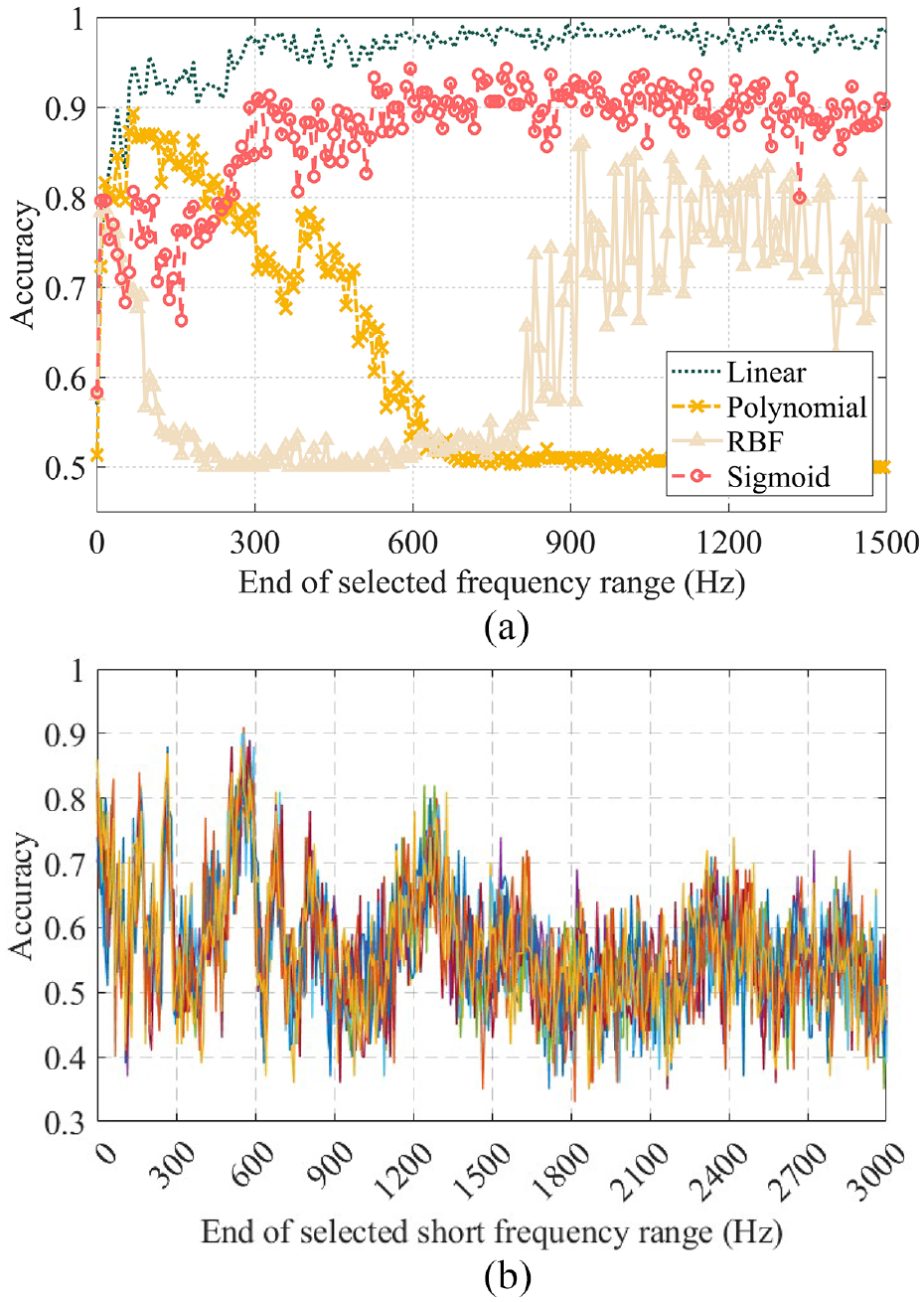
Selection of frequency ranges: (a) accuracy using frequency responses in different ranges and (b) accuracy using short-range frequency responses.
To investigate the distribution of bridge damage information in the high-frequency range, we tried to make classifications using just newly added short-range frequency responses. The frequency interval is selected as 7.63 Hz (100 frequency response points). In previous analysis, we utilize the increasing range, for example, 0–7.63, 0–15.26, 0–22.89 Hz, etc. Now, just newly added frequency ranges, such as 0–7.63, 7.63–15.26, 15.26–22.89 Hz, etc., will be employed for damage classification using the Linear SVM model. The classification results of 10 times random selection from case 0 (506 runs in total) are shown in Figure 9(b).
From Figure 9(b), we can see that, compared to Figure 9(a), the maximum accuracy decreases to 0.91 because just a few frequency responses are selected for classification. Once the bridge damage information is contained in that frequency interval, the damage detection accuracy will be relatively high (peaks), as seen in Figure 9(b). We can find that damage features are relatively dense in the range of 0–750 Hz. Also, it can also be noticed that damage features are distributed around 1300 Hz (obvious peaks) and 2400 Hz (weak peaks). After that, the accuracy is near 0.5, meaning that the SVM model cannot identify the bridge’s damage. Thus, the bridge’s damage features are densely distributed in the low-frequency range in this study. In the high-frequency range, the bridge’s damage features are sparsely disseminated, but they can still contribute to damage detection.
SVM using MFCCs
Using the vehicle’s frequency responses has been proved to be an effective way to classify healthy and damaged cases. However, the features input into the SVM model is boosted as the increase of the used frequency responses. For example, when selecting0–1000 Hz frequency responses as input, there will be 13,109 features. Even though the test accuracy can be enhanced, training SVM will become computationally expensive. Besides, if SVM with nonlinear Kernels is utilized, grid-search strategy needs to be used to find the best hyperparameters. The training efficiency is pretty low. Therefore, finding a suitable way to reduce the input dimensions is of great importance. Principle Component Analysis (PCA) is a very effective method used in SHM. 44 Employing PCA, the used frequency range 0–5000 Hz (65,537 features) in Section “SVM using frequency responses” can be decreased to 99 dimensions when the explained variance ratio (EVR) is 99.99%. However, the test accuracy using the four Kernels in SVM becomes 0.457 (Linear), 0.467 (Polynomial), 0.467 (RBF), and 0.467 (Sigmoid), respectively, and all results cannot reach 0.5. Thus, PCA may not suit the above problem well according to the test results. This paper utilized MFCCs to reduce feature dimensions and improve training efficiency. In the later discussion, all 0–5000 Hz frequency responses are used to calculate MFCCs because the high-frequency range (1000–5000 Hz) is typically represented as just a few MFCCs, and this will not impact the calculation efficiency.
Selection of filter banks’ number and SVM Kernel
Number of filter banks
When calculating MFCCs, the first step is to select a good number of filter banks (P in Equation (4)). In acoustic recognition, this number is typically chosen as between 22 and 40. But in bridge damage detection, the optimal number may vary. We employ 3–100 filter banks to perform damage detection problems. In this section, case 2 is used as an example to select the best number of filter banks, and all time-domain responses of the vehicle are regarded as one frame, namely
When Mel filter banks are evenly distributed in the frequency domain, the accuracy is plotted in Figure 10(a). We can see that when the number of evenly distributed banks is deficient, MFCCs cannot capture damage information in the frequency-domain responses. When the number increases to near 40, the accuracy becomes relatively stable. If better results are required, the number is expected to be more than 60. In comparison, if Mel filter banks are unevenly distributed, we can see from Figure 10(b) that, like the scenario using evenly distributed filter banks, a small number of the filter banks is not much effective for damage classification. However, when the number increases to 20, the classification performance using all four Kernels can reach good results. Using the uneven ones can save half number of filter banks used in damage detection. The main reason for the above phenomenon is that the latter concentrates on low-frequency responses but does not ignore the high-frequency range, while the evenly distributed filter banks treat all frequency ranges equally, thus more banks are needed to capture damage features in both low- and high-frequency ranges. Compared to evenly distributed Mel filter banks, MFCCs utilizing the uneven ones are computationally efficient since fewer features will be input into the SVM model. In the later analysis, the unevenly distributed Mel filter banks are employed. Furthermore, from Figure 10(b), we can also notice that the Polynomial and Linear Kernel’s performance is better than the others, and the Sigmoid Kernel shows the worst test accuracy. However, all Kernels can make the test accuracy more than 0.93. The contents related to Kernel selection will be discussed in Section “Kernel selection.” To maintain high accuracy, in this study, 61 filter banks that perform well on all Kernel functions are utilized.
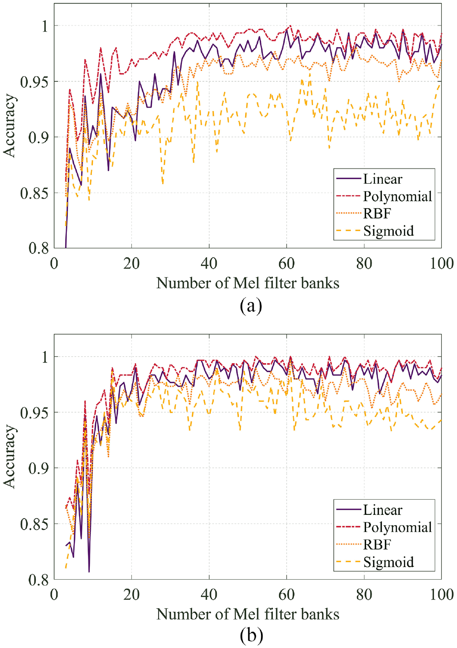
Selection of Mel filter banks: (a) evenly distributed Mel filter banks and (b) unevenly distributed Mel filter banks.
Kernel selection
As aforementioned, Kernel function selection is one of the most critical steps for training the SVM model. Case 0 and case 2 using different Kernels were discussed before. To select the best Kernel, the performance of four Kernels using one frame for all cases is shown in Table 4. The grid-search strategy is used for Polynomial, RBF, and Sigmoid Kernels to find the best test accuracy.
Accuracy using different time frames and different Kernels
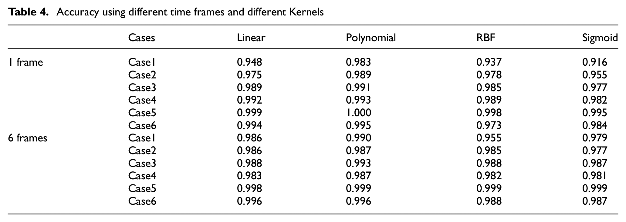
It can be seen from Table 4 that the test accuracy using different Kernels can reach at least 0.916. The Polynomial Kernel performs the best for all cases, and the next one is the Linear Kernel. However, as Table 1 shows, the Polynomial Kernel has four hyperparameters. Using the grid-search strategy will cost much time to find the best hyperparameters, especially when
As the Linear Kernel performs well for the damage detection problem, we believe that the datasets become linearly separable using MFCCs in the high dimensional space. For this reason, the dimensions of input features using MFCCs or frequency responses are reduced to three using PCA to make it into a 3-D space, as shown in Figure 11. Notice that the features are not explainable after PCA, so the numbers in axes are just featured values in low dimension space. It can be seen from Figure 11(b) that using MFCCs makes cases 1–6 separate from the undamaged case even though there are noised examples in case 0. Using frequency responses cannot separate case 0 and other cases linearly.
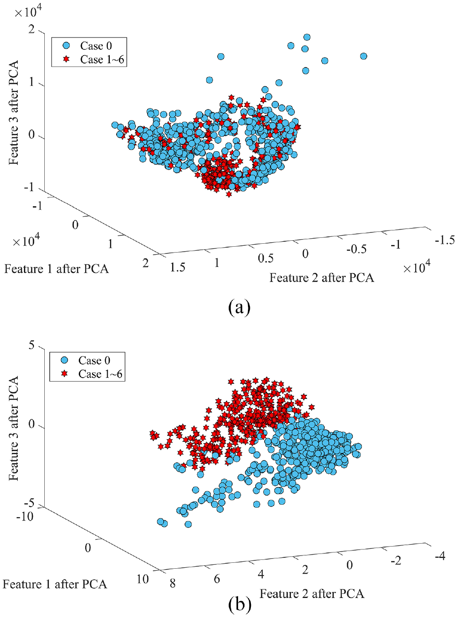
3-D comparison of using frequency responses and MFCCs. (a) 3-D visualization for frequency responses (0 – 5000 Hz) using PCA (65,537 → 3 dims, EVR = 0.353) and (b) 3-D visualization for 61 MFCCs using PCA (61 → 3 dims, EVR = 0.599).
MFCCs considering time frame
When
From Table 4, we can see that when different Kernels are employed for different cases, dividing the original signals in the time domain into six frames makes the damage detection accuracy better than just regarding all vibration data as one frame in most scenarios, especially for case 1 when the damage degree is relatively low. To investigate such a phenomenon, taking case 1 as an example, we analyzed 10 five-folder CV accuracies for random selecting 49 runs from case 0. It is noticed that when one frame is employed, the accuracy can be good or poor occasionally in 10 times random selection. However, employing six frames can always maintain good damage detection results. Therefore, six frames are employed in the later discussion.
Damage severity prediction
In previous discussions, it has been proved that the SVM model can classify intact and damaged cases using frequency responses and MFCCs with high test accuracy. However, in order to provide appropriate maintenance work, it is also important to detect the extent of damage (or damage degrees). For this reason, the damage severity prediction is investigated in this section. As shown in Table 2, all cases are labeled as classes 0–6. For case 0, 50 random samples out of all 506 samples are used to avoid the sample imbalance problem. Therefore, there are 340 samples and 366 features in total.
Because SVM is initially used as a binary classification model, there are two strategies when addressing multiple classification problems: one versus one (OVO) or one versus rest (OVR). OVO means that every two classes will be used to train an SVM model to find their decision boundary, and the OVR method is to regard one class as the first label and all the rest as the second label to train an SVM model. Since finding decision boundaries between every two cases is a special focus in bridge damage detection, OVO is employed in this study.
In the process of training and testing an SVM model, 50% of samples are used to train, and the rest are utilized for testing. Confusion Matrix, a generally utilized summary matrix of prediction results on a classification problem, is used in this paper to evaluate the trained SVM model’s performance. Figure 12 plots the confusion matrix for all predicted classes. The diagonal values mean that true and predicted labels are the same, so numbers in the diagonal are an accurate prediction.
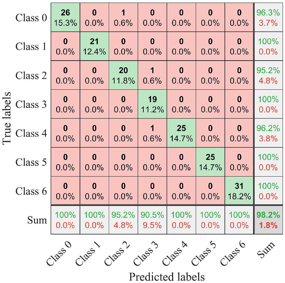
Comparison between true and predicted labels using heavy car.
From Figure 12, it can be seen that using the SVM model can classify different damage severity accurately. For those wrongly predicted labels, we notice that they are not far from the diagonal. It means that the SVM model will not make a big mistake when predicting damage severity. The predicted labels are around the true labels. Furthermore, it can be found that different damage cases are also linearly separable in Mel frequency space as the Linear Kernel is used to calculate the confusion matrix. Employing a 5-folder CV, the test accuracy ratio of the SVM model for multiple classifications is 0.962.
Influence on damage detection
Influence of the car’s weight
In the previous discussion, the heavy car in Table 2 is used. To investigate the influence of car’s weight, the car without extra weights is used in this section. Similar to Section “Damage severity prediction,” the confusion matrix is plotted in Figure 13.
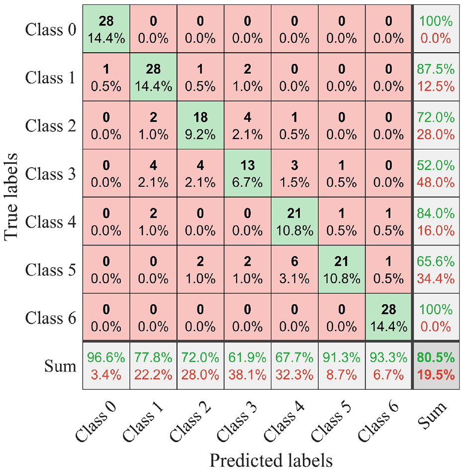
Comparison between true and predicted labels using normal car.
It can be seen from Figure 13 that when the normal car is used, the number of wrong predictions is increasing. But we can see that the false identification is still distributed around the diagonal. This means that the SVM model can distinguish a large part of damaged cases. After a 5-fold CV, the normal car’s overall test accuracy is 0.791. Therefore, to improve the accuracy of bridge damage detection, heavy vehicles are recommended in practical engineering.
Influence of damage severity and sample number
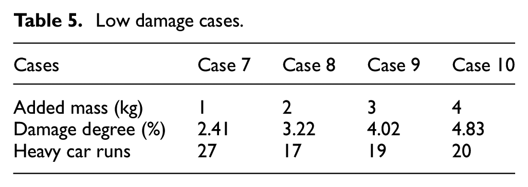
In this part, low damage severity with a limited number of samples is discussed. Cases with low damage degrees are shown in Table 5. Heavy car is used for low damage detection. For the bridge’s healthy state, 20 samples are randomly selected from 506 samples in case 0. The confusion matrix for predicting low damage cases are shown in Figure 14. We can see that low damage cases can be identified using the SVM model as well. But because the samples are relatively limited, the SVM model may not be able to learn the features of MFCCs completely, so there are some mistakes in predictions. The 5-folder CV result for low damage cases is 0.864.
Low damage cases.
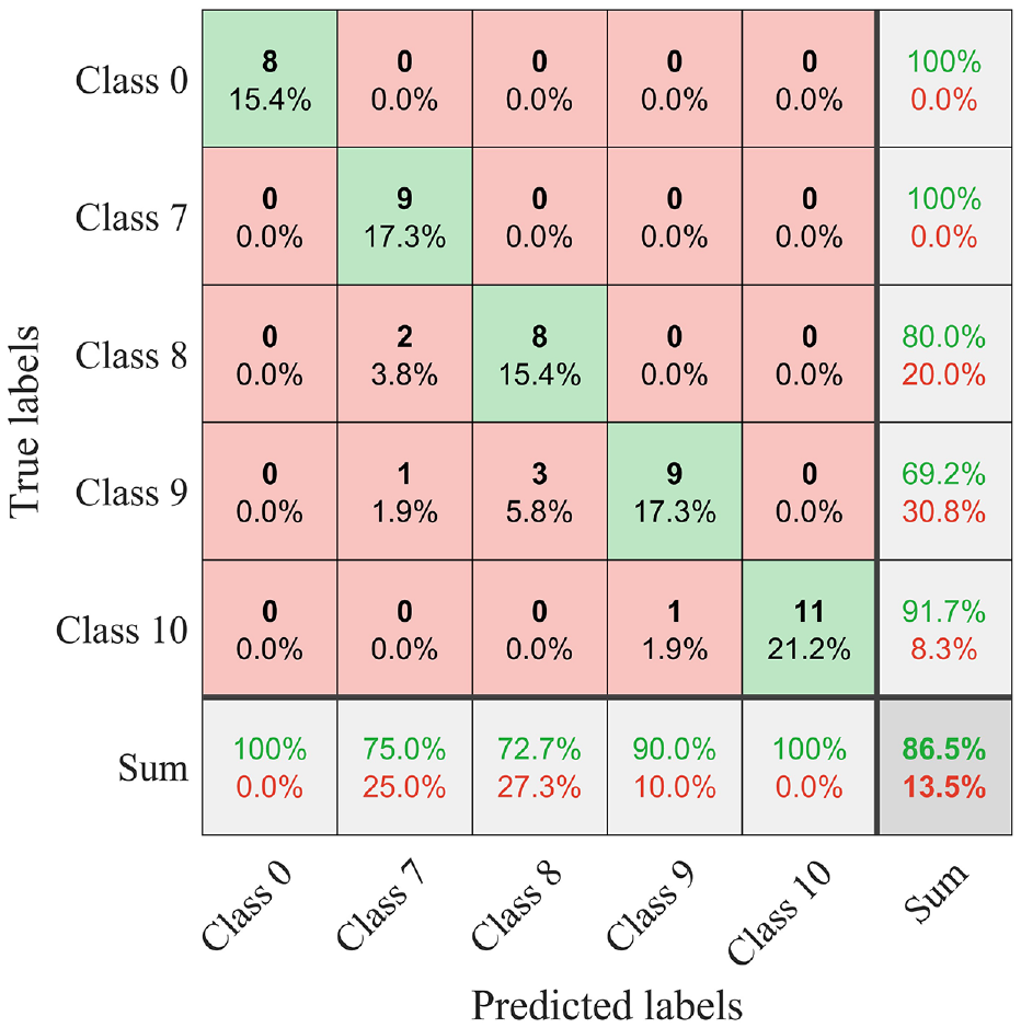
Comparison between true and predicted labels for low damage severity.
Conclusions and future work
This paper proposes a method to indirectly detect the bridge’s damage using drive-by vehicle’s vibration data, in which the frequency responses and MFCCs are utilized as damage indicators. MFCCs, initially used for acoustic recognition, were modified to suit the indirect bridge inspection method. Then, SVM is trained to identify the bridge’s damage. Trained SVM using MFCCs can detect the bridge’s damages with high accuracy. Laboratory experiments using a continuous bridge and a model car confirm the practicality of the proposed method. The main conclusion remarks are shown below:
The passing vehicle’s high-frequency responses also contain the bridge’s damage information and can play an important role in the bridge’s health assessment in addition to its low-frequency responses. With the increase in the utilized frequency range, the accuracy of damage detection will be improved until it becomes stable. Based on lab-scale experiments, the authors recommend using frequency responses within the 0–1000 Hz range for practical applications.
By transforming Hertz-scale frequency responses into MFCCs, datapoints of intact and damaged cases in the high dimension space become linearly separatable. Using MFCCs makes damaged cases easier to be detected by SVM models. The Linear Kernel is recommended for practical application since other Kernels depend on tuned hyperparameters heavily.
Compared to evenly distributed filter banks, the uneven ones need fewer banks to make the accuracy stable, thus can reduce the number of features fed into the SVM model. Also, dividing the original acceleration signals into several frames can improve the damage detection accuracy especially when the damage severity is low. The test accuracy is more than 96.2% for detecting different damage scenarios when 61 uneven filter banks and 6 frames are utilized in this paper.
The weight of the vehicle can affect the collection of the bridge’s dynamic properties, and the accuracy will be improved as the vehicle weight is increased. In practical bridge damage detections, a heavier car is recommended.
Despite the findings summarized above, there are still many factors that could negatively influence drive-by bridge damage detection procedures in actual conditions, such as the environmental noise, different passing traces, engine effects, etc. As the future work of this research, we will investigate the effects of real damages and different damage scenarios on the proposed method. In addition, influences of the bridge deck’s roughness and other ongoing traffic impacts on damage detection results will be checked by full-scale experiments with different modal parameters.
Footnotes
Appendix
Acknowledgements
The supports on the vibration tests provided by the staff of the laboratories in the Department of Civil Engineering and the Department of Mechanical Engineering at Aalto University are greatly appreciated.
Declaration of conflicting interests
The author(s) declared no potential conflicts of interest with respect to the research, authorship, and/or publication of this article.
Funding
The author(s) disclosed receipt of the following financial support for the research, authorship, and/or publication of this article: This study was fully financial sponsored by the Jane and Aatos Erkko Foundation in Finland (Grant number: 210018). Y. Zhang is financially supported by the Academy of Finland (Decision number: 339493).