The use of circumferential guided waves to monitor axial cracks in pipes

Abstract

Guided wave testing is in routine use to detect corrosion, particularly in the oil and gas sector, but the detection of axial cracking is difficult using the axially propagating waves commonly used for corrosion detection. This paper presents a novel guided wave monitoring technique for the detection of axial cracking in piping. Circumferential SH0 waves, travelling around the circumference were used in a monitoring configuration to detect axial defects in a 6 inch schedule 80 steel pipe. Finite Element (FE) analysis showed that both the defect reflection and the decline in the transmitted SH0 wave can be used for defect detection. Baseline subtraction was utilised to produce residual signals that can be better analysed for small defect reflections. The Root-Mean-Square (RMS) of the residual signal after baseline subtraction was found to be the most satisfactory means of monitoring defect progression. An amplification effect was identified where the residual signal is compounded by continued interaction with the defect on each revolution of the incident wave. The FE predictions were validated by an experiment in which an Electrical Discharge Machining (EDM) notch was grown in four stages. Temperature compensation using Location Specific Temperature Compensation (LSTC) was applied to the experimental data, allowing residuals to be compared for a ∼10 °C temperature swing over a monitoring period of over 2 months. It was determined that a 10 mm long (∼23% of wavelength), 5 mm deep (∼45% of the wall thickness) defect at an axial offset from the line of the transducers of 1.5 wavelengths (65 mm) would be readily detectable with a very high Probability of Detection (POD) and virtually no chance of a false call. Therefore, this novel guided wave monitoring system for axial crack detection is likely to be attractive for applications in a range of industries for its sensitivity to axial cracking combined with large coverage from a single transducer location.

Introduction

Thermal fatigue cracking is a major issue in pipe junctions which contain the mixing of high and low temperature fluids. The temperature changes in the pipe wall lead to cyclic thermal stresses which can initiate cracking and encourage propagation. ¹ Since the mixing of hot and cold fluids is a widespread practice in industry, the generation of thermal fatigue cracking is a common problem. For instance, in nuclear power generation, where safety standards are high and the cost of failure severe, thermal fatigue cracking is taken extremely seriously and every incidence of cracking is recorded and its progress in subsequent tests monitored. ²

Thermal fatigue cracks can form in different orientations based on the principal stress in the loading cycle. If hoop stress is the principal stress then an axial crack can form. ³ Although axial cracking is a considerable problem in pipe networks, the detection of small axial cracks is still a significant non-destructive evaluation (NDE) challenge. Traditionally, it has often been performed using manual bulk wave ultrasonic NDE methods such as time-of-flight diffraction (TOFD) from the exterior of the pipe. ⁴ However, this method is time-consuming as the inspected volume for a single test is small and the transducers must be repositioned for every test. It can also be difficult to achieve full coverage in more complex geometries.

To increase the speed of ultrasonic inspection, guided wave testing was developed in the 1990s.^5,6 Guided waves are a superposition of reflected bulk ultrasonic waves that form into wave packets that can propagate for large distances down a waveguide such as a pipe or plate. The main attraction of the technique is the full volumetric inspection of large geometries from a single transducer position which results in rapid and cost-effective inspection. Guided wave testing has been particularly successful commercially in the detection of corrosion in exposed and insulated pipelines. ⁷

The most common guided wave modes used for defect detection in piping are axially propagating fundamental pipe modes. Typically, the fundamental torsional mode T(0,1) is used as it is simple to excite and receive, non-dispersive and approximately uniform through the wall-thickness which allows equal detection capability for inner and outer wall defects. ⁸ The T(0,1) wave mode is usually excited by fixing a ring of transducers around the pipe circumference; these transducers then exert a circumferential force on the pipe which sends a wave propagating axially along the pipe, along the Z-axis in Figure 1. A pulse-echo configuration is common where the guided wave is sent along the pipe and any reflection produced is detected by the same ring. If a defect is present in the component, and the wave mode used exerts stress across the defect which produces a reflection, the time-of-flight and amplitude can then be used to locate and approximately size this defect. This is commonly used to detect corrosion patches in relatively simple pipe geometries; detection capability has been extended to more complex features such as tees and bends.^9–11 Research has shown an approximately linear relationship between the circumferential extent of a defect and the reflection produced by the defect. ¹² This has led to the T(0,1) wave mode being used in commercial applications for circumferential crack detection. However, the detection of axial defects using the T(0,1) wave mode has proven difficult, despite considerable research, ¹³ with the most successful attempts that use relatively high frequency pulses only able to reliably detect axial cracks which penetrate 75% of the wall thickness of the pipe. ¹⁴ Unfortunately, this sensitivity is still below most industrial crack detection requirements and the use of T(0,1) for axial defect detection has not seen commercial adoption.

Figure 1.

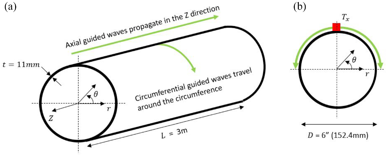
A schematic showing (a) the direction of propagation for axial and circumferential guided waves in a cylindrical geometry and (b) showing the circumferential guided waves travelling both clockwise and anti-clockwise around the circumference of the pipe.

This has led to interest in other guided wave modes for the detection of axial crack in piping. One proposal was to use the axially propagating flexural guided wave modes, which have some sensitivity to axial defects; however, in practice it is difficult to excite a single flexural mode and they all experience significant dispersion, which is a hindrance to easy adoption in practical NDE. ¹⁵ A substantially more promising method for axial defect detection is the use of circumferential guided waves. These are waves that can be excited from a single transducer and travel circumferentially in both directions around the circumference of a cylindrical waveguide, as shown in Figure 1. These circumferential modes are analogous to plate guided wave modes, the most widely studied being the fundamental Lamb modes S0 and A0 and the fundamental shear horizontal mode SH0. The behaviour of circumferential guided waves in hollow cylinders is dependent on the wall-thickness to radius ratio. ¹⁶ However, the majority of commercial piping have walls thin enough relative to their radius to use the plate mode approximation. ¹³

In an industrial context, some of the earliest applications of circumferential guided waves were by the US military who used circumferential Rayleigh waves to inspect the interior wall of artillery shells. ¹⁷ In the coming decades there was significant interest in using circumferential guided waves for the inspection of buried or insulated pipelines using ‘pigs’. This, in the context of NDE, is a device that is hydraulically pushed through the pipeline and used to inspect the pipeline for defects. Traditionally, ultrasonic (UT) ‘pigs’ used high frequency bulk wave ultrasound to scan the pipe wall as the pig moves through the pipeline. This inspection technique provides high accuracy and sensitivity to both cracking and corrosion. ¹⁸ However, in more complex geometries, traditional UT ‘pigs’ have difficulty in achieving sufficient coverage, often relying on multi-skip methods. These utilise shear waves that will reflect off several surfaces before they reach the desired inspection target. The reflections prior to interaction with the defect can lead to poor performance due to the considerable effect of surface features. ¹⁹ Circumferential guided waves offer a solution to this by giving significant volumetric coverage without the need for prior reflection. Guided wave UT ‘pigs’ were introduced in the mid-1990s and have seen significant commercial adoption as one of the most reliable axial crack-detection tools available today. ²⁰

Current commercial guided wave UT ‘pigs’ claim to be able to detect defects only greater than 15 × 1 mm, which is sufficient for pipeline inspection but not sufficient for the detection of thermal fatigue cracks in many cases. ²¹ Another issue with the use of UT ‘pigs’ is that they are only suitable for plain pipes without features such as reducers, perpendicular intersections or pipe-tees; hence their use is limited primarily to pipeline inspection. ¹⁸ Additionally, a UT ‘pig’ cannot be used as a monitoring system as the pig cannot be left within the pipe during operation without obstructing the pipe flow. There is therefore an acute demand in industry for a circumferential guided wave inspection system that can combine full volumetric coverage with sufficient sensitivity to detect small axial defects. A system that can be mounted on the outside of the pipe is also preferable as it would allow for more complex pipe features to be inspected.

This paper proposes to increase the sensitivity of circumferential guided wave systems to axial cracking by using it as a monitoring technique. In a monitoring system, the transducers are permanently fixed to the inspection geometry and take periodic measurements. ²² Baseline subtraction can then be performed on these measurements where every reading can be compared to the initial reading, which was taken when the structural condition of the component was known. The deterministic noise, known as coherent noise, can then be removed from the subsequent readings and any residual changes can be attributed to changes in the structural condition of the component. ²³ This has the potential to increase both the sensitivity and Probability of Detection (POD) of the inspection system.

However, a significant disruption to this method is changing environmental conditions, which alter the wave speed of the guided wave in the component. This can lead to residual signals that can either be mistaken for a signal produced by a defect or mask a defect signal. The simplest method to reduce this problem is the optimal baseline selection (OBS) method, where multiple baseline readings are taken in a range of environmental conditions. This allows the subsequent readings to be compared to a closer environmental match. ²⁴ However, even a small change in the environmental conditions produces a large change in the signal which quickly makes the method unviable due to the number of baseline signals required. ²⁵ An alternative to manually measuring several baselines is to try to account for the change in guided wave velocity by stretching, or compressing, the signal in the time domain. This method is called baseline signal stretch (BSS) which can be effective at small temperature fluctuations.^24–26 Yet there are substantial problems with this method, for instance, simply stretching the entire signal will alter the individual wave-packets which are unchanged by the changing temperature. ²³ Additionally, in practice, the changing temperature will also alter other factors in the monitoring setup, for example, the interface between the transducers and the pipe surface which can lead to changes in both the amplitude and the phase of the measured signal.^27,28 Location Specific Temperature Compensation (LSTC) was developed to try and compensate for these disparate effects and works by developing a calibration function, which is the relationship between signal amplitude and temperature for every possible point in the captured signal. This calibration function can be used to adjust the received signal before comparison with the baseline and has shown significant ability to reduce residuals in monitoring datasets which considerably increases detection sensitivity and the POD. ²⁹ For this paper, LSTC has been used on the experimental data as it is the most effective method to reduce residuals and boost the sensitivity of the monitoring dataset.

Mode selection is an essential part of guided wave testing and as touched on previously, there are four main guided wave modes used in circumferential testing for the detection of axial defects: S0, A0, SH0 and SH1.^16–30 For the detection of axial cracking in industrial applications, the shear modes are normally preferred over the Lamb waves as they experience less attenuation in coated or buried pipes. SH0 is the most commonly used, though there has been significant research into the use of both SH0 and SH1 for axial defect detection. There are distinct differences between the two modes, the most significant of which is the dispersion characteristics. The fundamental mode SH0 experiences very little dispersion even in curved geometries but the first-order mode SH1 experiences substantial dispersion in the frequency range commonly used for inspection. Despite its dispersive nature, SH1 is still used in industrial testing, mostly in UT ‘pigs’, as it is more sensitive to axial cracking than the SH0 mode, ³⁰ though it is often only suitable for applications which use propagation over only fractions of a revolution. ²¹ Therefore, for most applications, and in this paper, pure SH0 at frequencies below the frequency cutoff of SH1 is preferred for its simpler signals and ability to propagate with very little dispersion over long distances. For this application, using non-dispersive SH0 gives the possibility of capturing several revolutions of the wave around the circumference per test. This gives the opportunity for improved sensitivity due to multiple interactions with a defect, as every time the incident SH0 wave passes around the circumference it will hit the defect. Since the defect is in the same position, the defect reflection should compound with previous reflections and produce a larger signal relative to the incident SH0 wave.

Finite element study

In this study, a 3D Finite Element (FE) analysis was used to characterise the behaviour of the guided wave monitoring system. The mesh was generated manually using MATLAB ³¹ and the initial pre-processing was also performed in MATLAB. The simulation was solved using the explicit time domain FE solver Pogo ³² developed at Imperial College London, and the post-processing was performed primarily on MATLAB with visualisation performed using PogoPro ³³ and Paraview. ³⁴

The model was a 3 m long, 6 inch nominal bore schedule 80 pipe with a wall thickness of 11 mm. A 3 m long section was modelled with the transducer position in the middle (L = 1.5 m) so that multiple circumferential transits were seen before the appearance of end reflections. The mesh was structured with eight-node 1 mm general-purpose brick elements with reduced integration (C3D8R). ³⁵ Three-cycle Hann-windowed pulses with a range of centre frequencies from 55 to 95 kHz were used in the experimental testing; however, the middle of the range 75 kHz is presented in the FE section of this paper. The main mode of interest is the SH0 mode propagating circumferentially and given its velocity of 3260 m/s, the mesh size gave approximately 34 nodes per wavelength at the highest frequency. Previous FE studies have recommended anything from 10 nodes per wavelength, ³⁶ up to 20 for brick elements, ³⁷ so the mesh generated for this model will capture the wave behaviour accurately. The cutoff frequency of the SH1 mode in the 11 mm wall thickness is 157 kHz, so this mode is not excited. The relevant material properties of the pipe are a Young’s modulus of 203 GPa, a density of 7850 kg/m³ and a Poisson’s ratio of 0.275.

The transducers used in the experiments exert an axial force on the outer wall and have a small contact area so they can be modelled by exciting a single node in the axial direction. Figure 2 shows a snapshot of the displacement field generated by the source. The SH0 mode can be seen propagating circumferentially, the amplitude reducing with angle to the circumferential direction, reaching a null in the axial direction where the S0 mode can be seen; the slower A0 mode is also excited with a maximum in the axial direction but this is not separated from the SH0 signal.

Figure 2.

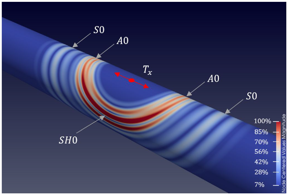
The field of the normalised magnitude of the displacement showing the circumferential SH0 waves and also the axial S0 and A0 waves that are excited when shearing the node at the position Tx (the size of Tx has been exaggerated for visibility). Displacement values below 7% are excluded to make the significant waves clearer.

Figure 3 shows the pulse-echo signal from a receiver position coincident with the source. Three circumferential passes of the SH0 mode are observed before the appearance of an S0 reflection from the end of the pipe. The pulse-echo configuration ensures the clockwise and anti-clockwise SH0 waves constructively interfere at the receiver node position and appear as a single wave in Figure 3. This is also true for the S0 wave arrival, as the source node is at the axial midpoint of the pipe, so the S0 pipe end reflections will arrive at the same time. Therefore, each wave labelled is a superposition of two waves. The decline in the normalised amplitude of the SH0 arrivals is entirely due to the beam spread of the SH0 wave as it travels around the circumference as there is no material attenuation built into the model. This can be seen in Figure 2, where beam spread of the SH0 wave is already significant after a quarter rotation.

Figure 3.

An A-scan of the defect-free signal in a pulse-echo configuration. The SH0 waves are labelled with the format $\mathrm{SH}{0}_n$ where n refers to the number of revolutions around the circumference. The x-axis is the number of circumferences the SH0 wave has travelled and the y-axis is normalised to the maximum magnitude of the first arrival of the SH0 wave. The exponential decay curve, calculated using the Hilbert envelope of a model with the end reflections removed, fitted to the SH0 arrivals is used to apply distance–amplitude correction (DAC) in Figure 6.

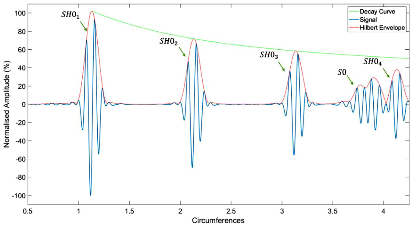
Figure 4 shows the same test as Figure 3 with an 8 × 4 mm defect inserted 90° away from the transducer circumferentially in the anti-clockwise direction. This corresponds to a quarter circumference and therefore the reflections from this defect will arrive half a circumference after the incident SH0 wave. The initial defect reflection (D₀) is produced by the initial SH0 wave ( $\mathrm{SH}{0}_0$ ) which is not shown; it occurs after 0.5 circumferences. The defect was created by duplicating the nodes on the crack face and then changing the element connections so that the elements on one side of the crack are connected to the new duplicated nodes. This creates a crack with zero-volume, which has been used extensively in ultrasonic modelling to simulate natural cracks. ¹² The defect reflections are significantly smaller than the SH0 waves that produced them and they would be difficult to detect by just analysing a single A-scan, as shown in Figure 4.

Figure 4.

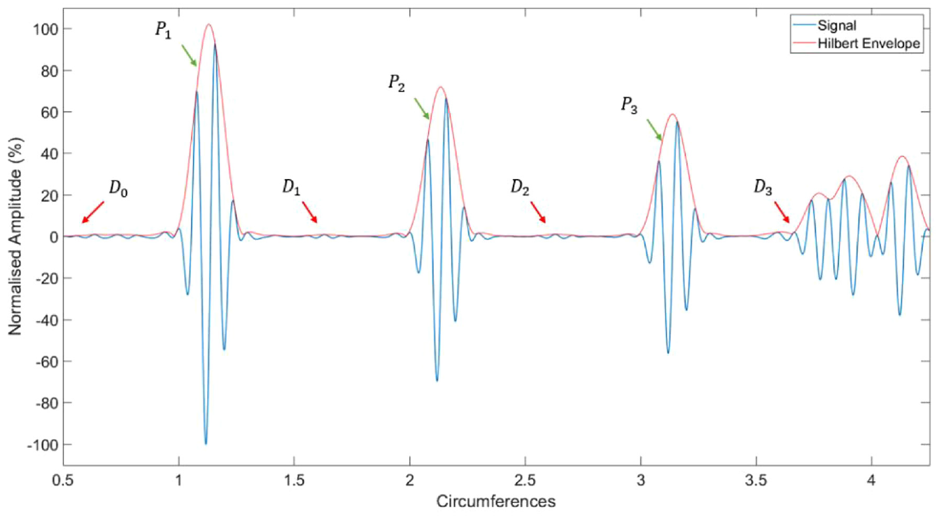
An A-scan of the signal with a defect in a pulse-echo configuration. The reflections from the defect after it has interacted with the SH0 wave are labelled with D_n, where n refers to the previous SH0 wave. The exception is $D_0$ which occurs after the initial SH0 wave. The peak of the Hilbert Envelope for each revolution is labelled with the format $P_n$ , the ratio of $P_3$ / $P_1$ is used in Figure 8.

The change produced by the defect is seen more clearly if the defect-free signal of Figure 3 is subtracted from the signal with the defect present inFigure 4 to give the residual signal shown in Figure 5. Successive defect reflections can be seen, including $D_3$ that was obscured by the S0 arrivals in Figure 4. The amplitude of the propagating SH0 wave is reduced by the defect and this change is shown by the I signals in Figure 5. Note that the defect was placed at 90° as it gives the largest separation between the I and D waves for illustrative purposes; for defects in other positions there may be overlap between the I and D waves. Overlap of the I and D waves does not affect detectability but the 90° case is the simplest example and is used here to facilitate explanation of the wave interactions.

Figure 5.

The residual after the subtraction of Figure 3 from Figure 4. I waves represent the decrease in the SH0 wave after interacting with the defect and the D waves are the reflection from the defect. Note the different scale on the y-axis when compared to Figures 3 and 4.

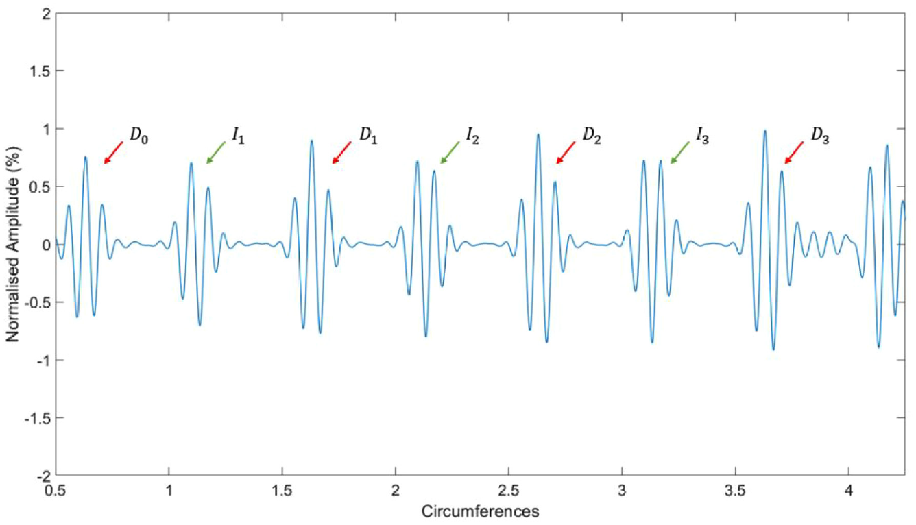
All the defect reflections are superpositions of reflections caused by the clockwise and anti-clockwise SH0 waves, except for $D_0$ which is the first reflection of the anti-clockwise SH0 wave. This is a consequence of the defect placement at 90°; if another circumferential position was chosen then there would be two distinct defect reflections.

Successive defect signals and changes in the SH0 wave amplitude are roughly constant in Figure 5, in contrast to the decay due to beam spreading seen in the original signals of Figures 3 and 4. This is due to the propagating SH0 wave interacting with the defect on each circumferential transit. If DAC is applied to the signals of Figures 3 and 4 using the decay curve fitted to successive peaks shown in Figure 3, the change in residual signal increases with time as shown in Figure 6. This suggests that it may be beneficial to analyse the whole residual signal, rather than just the initial arrivals, though the length of signal that it is beneficial to analyse will depend on the random noise floor.

Figure 6.

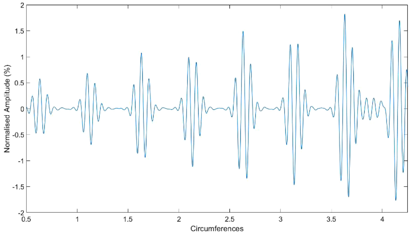
The residual presented in Figure 5 with DAC applied to show the increasing defect reflection if the beam spread due to attenuation is removed.

The beam spread of the SH0 wave can potentially be used to detect defects which are offset axially from the transducer and a pair of residuals is shown in Figure 7 for defects at different axial offsets. The amplitudes of these residuals are lower than the equivalent reflections from an in-line defect, with the exception of $D_0$ in the $1\lambda$ offset case which is larger than the in-line equivalent; this is because the defect is one wavelength (43.5 mm) away from the centre line and a quarter circumference (137 mm) around the pipe from the transducer. It is therefore at an angle of 17° to the circumferential direction, so significant amplitudes of the A0 and S0 modes seen in Figure 2 interact with the defect and increase the size of the reflection. The wave velocities are different, so the pulse appears longer than the other reflections. This effect is much diminished in later reflections as the effective angle of incidence is reduced as the propagation distance around the circumference increases. Additionally, the axially propagating S0 and A0 waves, which are identified in Figure 2, will produce reflections from the defect that will interfere with the reflections from the circumferential SH0 wave. However, this effect is isolated to the start of the test as the A0 and S0 modes travel away from the defect and only return as pipe end reflections after several revolutions of the SH0 circumferential wave.

Figure 7.

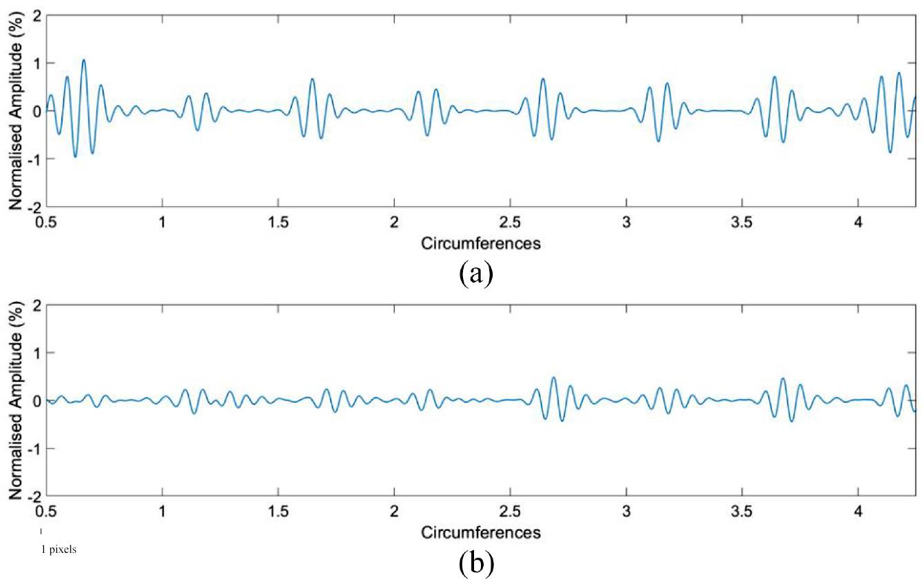
The residuals defects offset axially from the transducer by (a) 1 $\lambda$ (43.5 mm) and (b) 3 $\lambda$ (130.5 mm). $\lambda$ is the wavelength of the incident SH0 wave.

The results presented in Figure 7 display promising detection capabilities for axially offset defects and this is quantified in Figure 8 with a range of defect sizes and axial offsets. The crack-like defects are all in the axial-radial plane so they are normal to the circumferentially propagating SH0 wave; they are rectangular with a 2:1 ratio between their axial extent and depth. Two defect detection methods are presented; the Root-Mean-Square (RMS) of the residual and the percentage change of the ratio of the first and third arrivals of the SH0 wave. The RMS of the residual is a common method for defect detection in monitoring and is advantageous since, as shown in Figures 5 and 7, change occurs over a large fraction of the signal and the method avoids potential issues with random fluctuations at a single point; it is also the basis of temperature compensation methods such as optimum baseline subtraction ²³ and BSS. ²⁴ The ratio of successive SH0 arrivals is obtained by taking the Hilbert transform of the received signal and computing the ratio of the amplitudes of different arrivals, as shown in Figure 4. This method is effectively self-calibrating^38,39 as, unlike the residual computation, it does not depend on the transducer output being stable in time.

Figure 8.

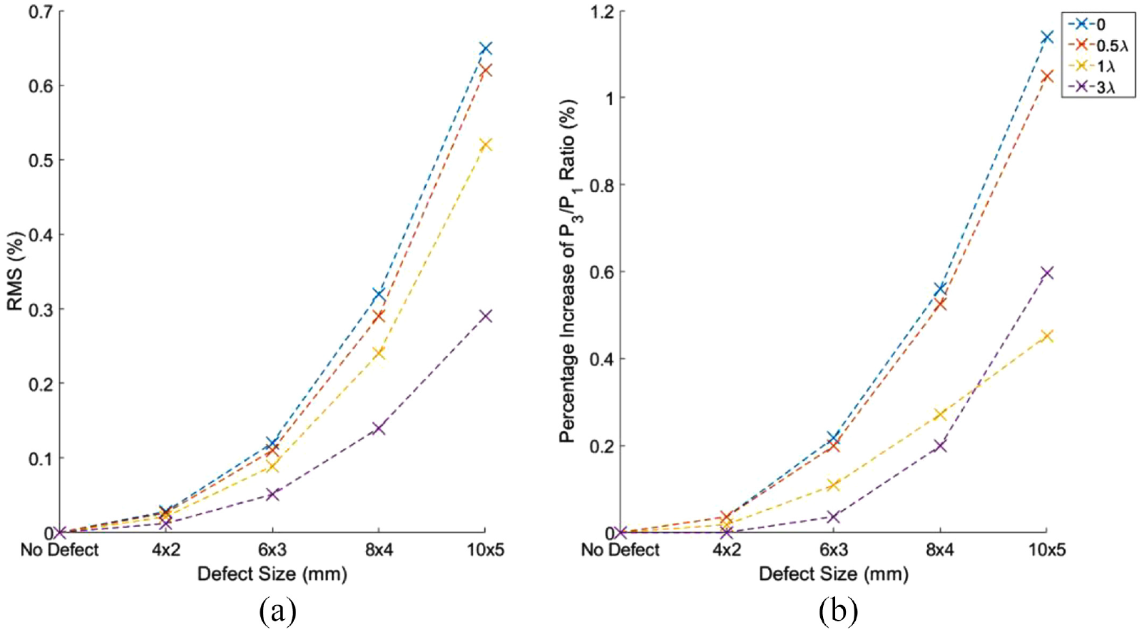
Damage detection metrics versus defect size for a range of axial offsets where $\lambda$ = 43.5 mm. (a) the RMS of the residuals and (b) the percentage increase of the ratio of the maximum values of the first and third SH0 arrivals. The base residual for the P₃/ $P_1$ ratio is 0.553. Note the different y-axis scales.

Two main trends are clear in Figure 8(a): the RMS of the residual increases as the defect size increases and increasing the axial offset decreases the RMS of the residual. Figure 8(b) shows that the percentage change in the ratio of the third to first circumferential SH0 arrival also increases as the defect size increases. The increase in the $1\lambda$ offset curve is slower at larger defect sizes than the other cases; this was found to be due to multiple reflections from the larger defects superposing on the main SH0 arrivals and so affecting the signal envelope.

All the results presented thus far in this section have had the transducer and receiver modelled in the same position in a pulse-echo configuration, the simplest example of this is seen in Figure 3. A pulse-echo configuration gave the simplest signals to analyse the behaviour of the system and illustrate the different waves present. However, a pitch-catch setup was used in the experimental validation presented in the next section to boost sensitivity, remove an initial dead-zone where any signal is masked by the excitation pulse and stabilisation of the receiver amplifier after the excitation pulse. A pair of defect-free examples are shown in Figure 9 with the receiver moved 30° and 60° clockwise around the circumference from the transducer; in contrast to Figure 3 the separate arrivals of the clockwise (C) and anti-clockwise (A) arrivals can be seen and the test has been extended to include the initial clockwise SH0 wave (C₁). The different receiver positions are chosen to clearly show the change in arrival times of the $C$ and $A$ arrivals due to the moving circumferential position. The pitch-catch examples are normalised to the maximum of the first SH0 arrival in Figure 3 to allow direct comparison. Due to the different travel distances, the clockwise and anti-clockwise pairs are significantly separated on each transit, for example, 30° versus 330° for $C_1$ and $A_1$ respectively in Figure 9(a). The beam spread of the SH0 wave discussed previously is also clearly visible when comparing the two cases presented in Figure 9 as $C_1$ is larger in the 30° case than its equivalent in the 60° case and the opposite is true for $A_1$ .

Figure 9.

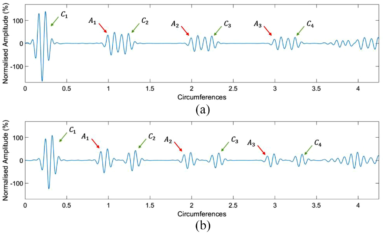
Pitch-catch results for the defect-free case showing a receiver at (a) 30° and (b) 60° with two SH0 arrivals visible in both cases per revolution. Note the different scale on the y-axis to Figure 3.

Experimental validation

The experimental setup used to record the guided waves is shown in Figure 10. The test component was a 3 m long, 6 inch nominal bore schedule 80 pipe made of 304 L stainless steel; the dimensions are shown in Figure 1. The pipe is supported by two vee-blocks at the ends of the pipe with the surfaces of the vee-blocks padded with synthetic rubber to create an acoustically soft interface between the pipe and the support to prevent unwanted reflections.

Figure 10.

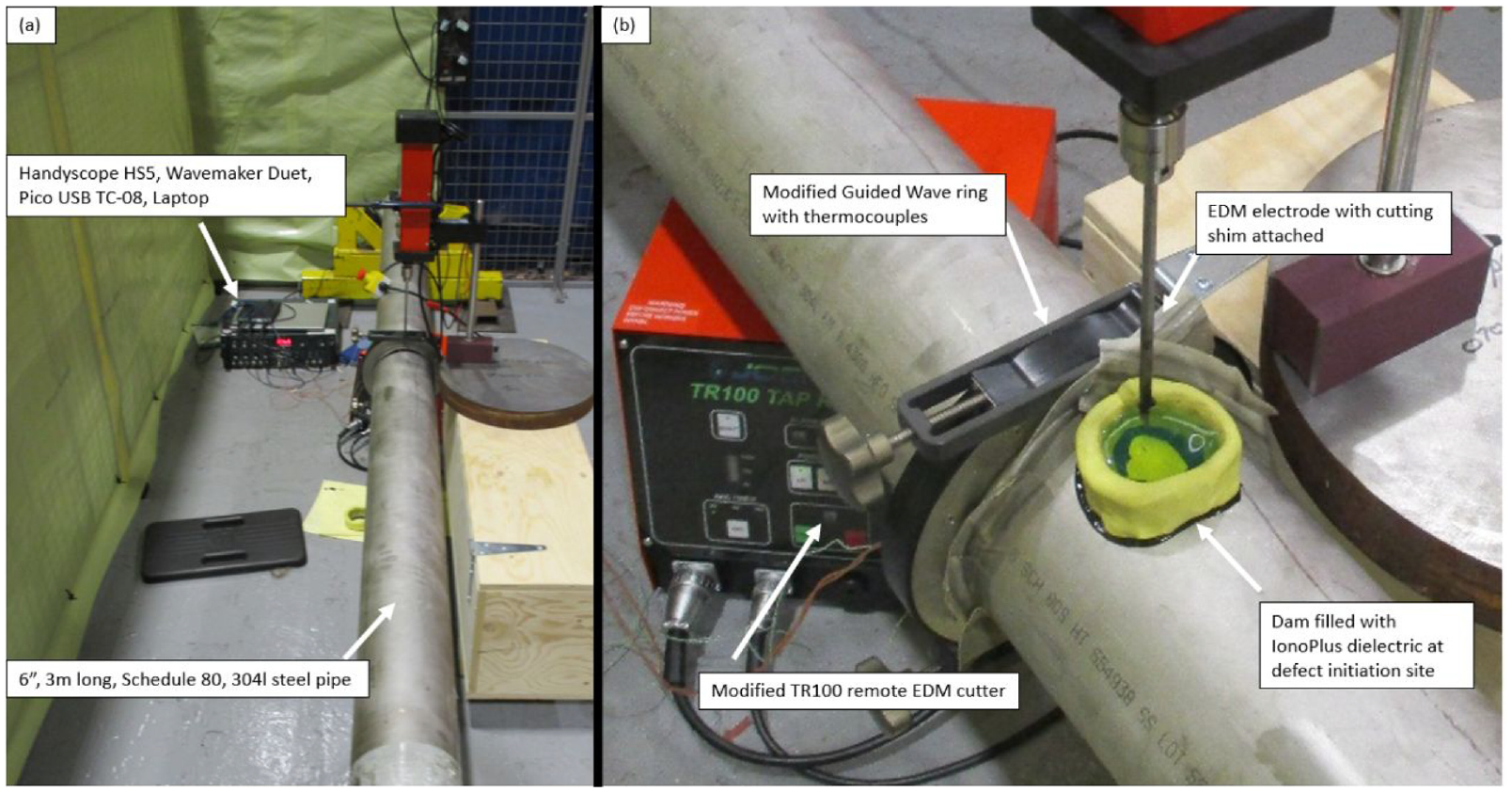
Photograph of the EDM cutting setup on the pipe showing the (a) full equipment and a (b) close-up of the cutting location. Most important constituents of the experimental setup are labelled with the only exception the second vee-block and the grounding cables attached to the end of the pipe that are obscured by the remote EDM head. The Dam used to hold the IonoPlus dielectric fluid ⁴⁰ was removed after each defect cut.

To generate the circumferential guided waves, a guided wave ring provided by Guided Ultrasonics Ltd. was used. ⁴¹ This ring was designed for axial testing where it would generate a T(0,1) guided wave by shearing the pipe in the circumferential direction with multiple transducers around the circumference. This form of guided wave ring requires no lubricant and is simply clamped onto the pipe to form a dry-coupled connection. To modify this ring to generate circumferential guided waves, two transducers were made with the piezoelectric crystal rotated 90° so they sheared along the pipe rather than circumferentially, as shown in Figure 2. These were then placed in the ring with 50° of separation which is the maximum separation possible with the current ring design; a schematic of the ring is shown in Figure 11. The remaining transducers were removed and dummy transducers made of acoustically soft material were put in their place. As mentioned previously, a pitch-catch configuration was used to minimise the noise floor, reduce the ‘dead-zone’ and allow stabilisation of the amplifier after the excitation pulse. The temperature of the pipe was recorded during every measurement using a Pico USB TC-08 data logger with two thermocouples attached to the pipe surface by placement underneath a dummy transducer at 180° separation.

Figure 11.

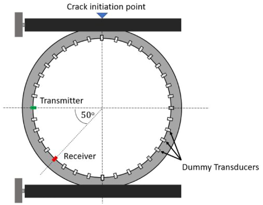
A schematic of the Guided Ultrasonics Limited guided wave ring used to generate the SH0 circumferential guided waves. The large blocks on either side of the ring represent the clamps used to attach the ring to the pipe. Crack initiation point is axially offset from the transmitter and receiver by 1.5 $\lambda$ , as seen in Figure 10(b). The ring is shown in the same orientation as in Figure 10 to aid understanding.

A Handyscope HS5 waveform generator was used to generate the 3-cycle Hann-windowed pulse and a range of centre frequencies from 55 to 95 kHz in intervals of 10 kHz was tested. ⁴² The middle of that range, 75 kHz, is presented in this section, as it was in the modelling section of this paper. A Wavemaker Duet (Macro Design) was used as both an input and output amplifier. ⁴³ A slot simulating a crack was initiated on the pipe surface approximately 1.5 $\lambda$ (65 mm) away from the transducer with initial target dimensions of 6 mm axial extent and 3 mm in depth (6 × 3 mm). This slot was then expanded to 10 × 5 mm and then 14 × 7 mm, simulating the growth of a single crack. The actual dimensions for the slots were: 6.4 × 3.0, 9.9 × 5.9 and 13.9 × 7.2 mm. The gape for each of the defects was expected to be 0.5 mm; however, the gape for the 14 × 7 mm defect increased to approximately 0.65 mm due to the multiple cuts needed to achieve the target depth.

The crack was created using an Electrical Discharge Machining (EDM) machine to create a realistic defect by spark eroding the slots. EDM slots are commonly used as artificial defects to mimic fatigue cracks in ultrasonic testing and they produce broadly representative reflections. ⁴⁴ However, the amplitude of the reflection is often higher than an equivalent thermal fatigue crack and this should be accounted for in practical application of this system.^45,46 A TR100 remote EDM machine produced by Eurospark was used to cut the imitation defects for this experiment. ⁴⁷ A TR100 is not intended to be used to machine precision slots like those achieved in this experiment. However, modification was performed by the Rolls-Royce NDE Development Division by attaching a micrometer to the internal feed mechanism and an external digital display that tracked the feed distance, allowing for better depth control.

The experiment ran for 57 consecutive days with a reading taken approximately every 7 min, leading to more than 11,000 individual readings. The component was kept in a large heated indoor space for the entirety of the experiment and the temperature fluctuated between 17 °C and 27 °C. The laboratory that the experiment took place in was heated during the day, leading to periods when the temperature of the lab rose quickly and the pipe temperature was not stabilised. To remove this issue, only measurements acquired between 7 pm and 7 am were used for the analysis shown in this paper, as at that time the laboratory was cooling naturally. Additionally, LSTC is more effective if the temperature is consistent throughout the component and the most likely period for this is the cooling cycles overnight. ²⁹

The experimental dataset can be split into five chronological monitoring periods which are identified on Figure 12. The initial monitoring stage was the ‘Baseline’ period recorded before any defect cut took place; this was used as the baselines for Baseline Subtraction and LSTC temperature compensation as discussed in the Introduction. It can be seen on Figure 12 that the baseline period has a greater range of temperatures than the subsequent monitoring periods; this was done deliberately to improve the LSTC in which it is advisable to have baseline results with a greater range of temperatures than the results being investigated. ²⁹ The next monitoring stage was the ‘noD’ (no defect) period, which was recorded before the initial defect cut but after the baseline period. This was used to provide a control measurement for the sensitivity of the system. The final three regions refer to the monitoring periods for the three defect sizes tested in this experiment and are labelled according to the dimensions of the EDM slot. The periods are not in uniform length, due to a number of practical factors such as technician time and space requirements in the laboratory.

Figure 12.

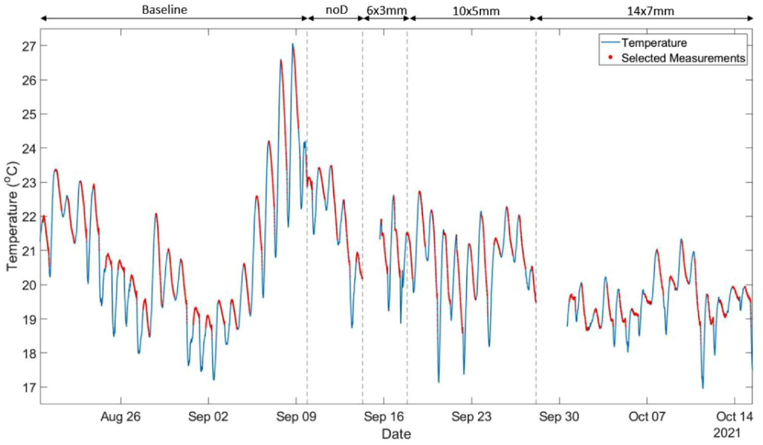
The temperature of the experiment throughout the entire monitoring period. The blue line is the recorded temperature and the readings between 7 pm and 7 am are highlighted in red. Also marked on the figure is the start/end of the different monitoring regions. Note the gap after the 6 × 3 mm cut and the 14 × 7 mm cut, the first gap was a power cut and the second resulting from the long cutting time required for the 14 × 7 mm defect.

The capture period for each signal allowed 10 full revolutions of the SH0 wave to be seen; however, after approximately 3.5 revolutions the signal becomes increasingly noisy because of the recurring pipe-end reflections that have been discussed previously in this paper. This can be seen in Figure 13(a) with the initial S0 end reflection arriving at approximately 3.75 circumferences. The region before 0.5 circumferences is characterised by a large ringing effect from the excitation pulse and is excluded from analysis. Due to the increased complexity after 3.5 circumferences the analysis of this experiment in this paper was confined to the initial portion of the capture period from 0.5 to 3.5 circumferences.

Figure 13.

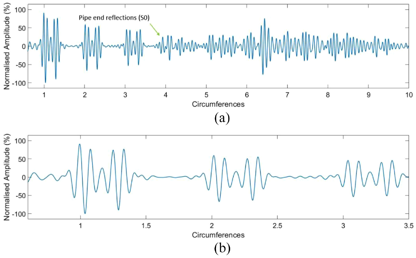
A sample signal from the ‘Baseline’ monitoring period. The excitation was a three cycle Han-windowed pulse with a centre frequency of 75 kHz. (a) shows the entire capture period with (b) showing the initial section before the arrival of the pipe-end reflections. A band-pass filter with upper and lower bands of 50 kHz and 100 kHz has been applied to these signals. The results are normalised to the positive peak of the magnitude of the initial SH0 wave.

An example experimental signal and residual from the 14 × 7 mm monitoring period is shown in Figure 14. As a pitch-catch configuration was used in the experimental validation, the anti-clockwise and clockwise arrivals can clearly be identified as predicted in the FE study. The residual is more complex than those shown in the FE study; this is primarily due to the pitch-catch configuration but also due to the coherent noise inherent in the experiment. The continuous nature of the residual strongly suggests that both the I and D waves already identified from Figure 5 are present. Additionally, the residual does not experience a significant drop in amplitude over the 3.5 circumference period, implying the amplification effect identified in the FE study is also present.

Figure 14.

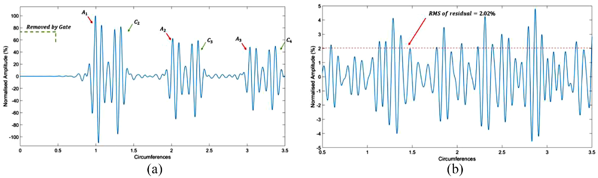
An example of an experimental (a) signal and (b) residual from the monitoring period where the 14 × 7 mm defect was present. The signal (a) shows 3.5 circumferences of the clockwise and anti-clockwise SH0 waves. The initial 0.5 circumferences contained a dead-zone due to cross-talk between the transducers and this region is removed by a gate. Plot (b) shows the residual of the signal in (a) after LSTC is applied. The RMS of the residual value is plotted in (b) as a red dotted line. The initial gated period is not shown in the residual signal in (b).

As discussed previously, the RMS of the residual is the preferred method for quantifying the performance of the signal as the ratio method can have unpredictable results at larger axial offsets. In this case the axial offset is 1.5 $\lambda$ and therefore only the RMS of the residual is considered. The residuals were obtained using LSTC on the BSS-compensated signals. After the residuals have been obtained and post-processing is performed, the RMS of the residual can be calculated for every residual in the monitoring period. If they are then grouped in the chronological monitoring periods shown in Figure 12, excluding the ‘Baseline’ period, then a graph showing the sensitivity of the system to different defect sizes can be produced, as shown in Figure 15.

Figure 15.

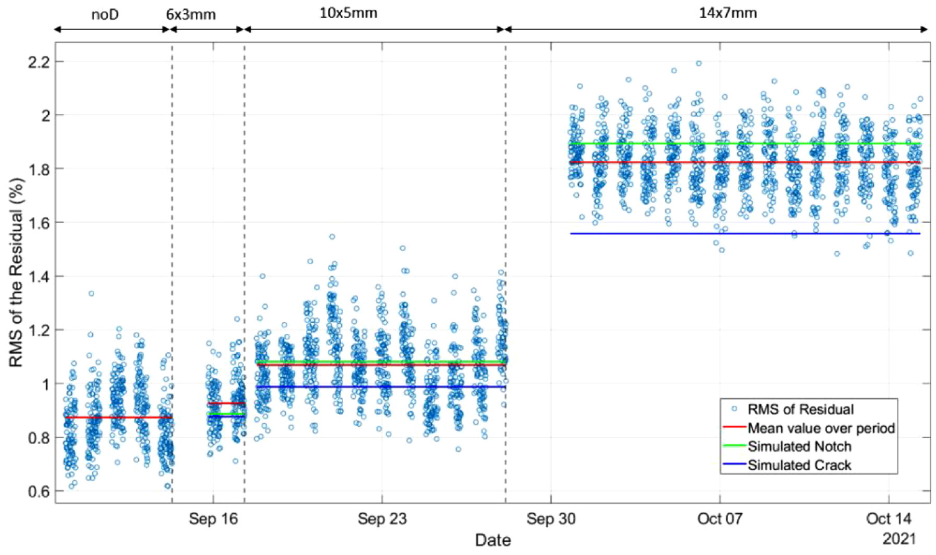
Experimental results after post-processing for the portion of the capture period − 0.5 to 3.5 circumferences. Each point represents the $\mathrm{RM}{\mathrm{S}}_{\mathrm{DN}}$ of a single residual and the red lines are the mean values of all RMS of the residuals in each monitoring period. The dotted lines represent the different defect cuts in the same manner as Figure 12. Results for a simulated notch and crack are also displayed and converted to $\mathrm{RM}{\mathrm{S}}_{\mathrm{DN}}$ .

The 6 × 3 mm monitoring period was unfortunately short due to the practical limitations mentioned previously. Despite this, even with only two days of data an increase in the RMS of the residual was observed. The gaps present in the data are due to the readings from 7 am to 7 pm being excluded due to irregular heating in the laboratory as mentioned previously. There are two more significant gaps in the data after the 6 × 3 mm and 14 × 7 mm cuts; these are due to a power cut and extended cutting time as mentioned previously. As can be seen from the ‘noD’ period, there was a significant residual signal before any defects were introduced with a mean RMS value of 0.87% of the peak of the first circumferential SH0 arrival. This is due to the unavoidable presence of random measurement noise in the residuals after temperature compensation, possibly summed with other noise components such as: imperfect temperature compensation due to non-uniform heating or sensor drift from either the amplifier or sensor drift from either the PZT transducers or the electronic components driving the excitation/reception of the signals (i.e. a progressive change in the frequency response function of any of the formers). Note that no efforts have been put to optimise the hardware components used in this experimental campaign; hence it is possible that a more careful choice of, for example the amplifier, can result in better signal stability.

Figure 15 also displays the results from FE analysis performed to validate the results presented earlier in this paper. Two simulated defect types were used in predictions, a notch and a zero-volume crack. The simulated notch was created by deleting 0.5 mm C3D8R cubic elements until the correct shape and dimensions to match the experimental EDM notch was achieved. Zero-volume cracks were used to generate the crack results seen in Figure 15 and the method to generate this type of simulated defect by decoupling nodes is the same method already described in this paper in a previous section.

The results from the simulated notch are not directly comparable with the experimentally measured values as the former are devoid of noise. The experimental results can be thought of as a combination of a defect-induced RMS value and a noise-induced RMS value. Therefore, the RMS of the experimental signal can be expressed mathematically as:

$$\mathrm{RM}{\mathrm{S}}_{\mathrm{DN}}=\sqrt{\mathrm{RM}{{\mathrm{S}}_{\mathrm{D}}}^2+\mathrm{RM}{{\mathrm{S}}_{\mathrm{N}}}^2}$$

(1)

where RMS_D is the RMS purely due to defect reflections existing in the signals and $\mathrm{RM}{\mathrm{S}}_{\mathrm{N}}$ is the RMS solely due to the measurement noise sources discussed previously, and thus $\mathrm{RM}{\mathrm{S}}_{\mathrm{DN}}$ represents the RMS of the residuals of the signal containing both defect reflections and noise. For the purpose of comparing the experimental and simulated results, the experimental $\mathrm{RM}{\mathrm{S}}_{\mathrm{N}}$ value for the noD monitoring period can be added to the simulated $\mathrm{RM}{\mathrm{S}}_{\mathrm{D}}$ value for each defect size; in this case the $\mathrm{RM}{\mathrm{S}}_{\mathrm{N}}$ value is 0.87%. This value can then be directly compared to the $\mathrm{RM}{\mathrm{S}}_{\mathrm{DN}}$ value obtained during the experiment and shown as the horizontal red lines on Figure 15.

The RMS of the residual showed a seemingly quadratic growth on Figure 15, which equates to an approximately linear growth when compared to the area of the defect. This is consistent with Figure 8(a) and was predicted by the FE validation for both a simulated notch and crack. However, the crack has a noticeably lower increase in $\mathrm{RM}{\mathrm{S}}_{\mathrm{DN}}$ and the simulated notch proved to be a much better predictor of the experimental results. This is likely due to the axial gape, which is zero in the case of the simulated crack and matches the experimental axial gape of 0.5 mm in the case of the simulated notch. Notches with axial gapes below 0.25 λ, in this case approximately 11 mm, should result in larger reflections from an incident SH0 wave than the equivalently sized crack, ¹² and this is observed at every defect size. The predicted notch results generally agree well with the experiments apart from the small defect case where the predicted reflection is small compared to the noise and the monitoring period was relatively short.

The four sets of RMS values of residuals for the monitoring periods shown in Figure 15 were analysed to assess whether they appear to be normally distributed. For illustration, Figure 16 shows a histogram of the distribution for to the noD monitoring period. All four datasets failed the Kolmogorov–Smirnov normality test with test significance set at 5% suggesting that noise components other than random measurement noise are also likely present in the residuals. ⁴⁸ As mentioned previously, this could also be due to drift and/or instability effects caused by the equipment used in this experiment; therefore it is possible that this can be improved.

Figure 16.

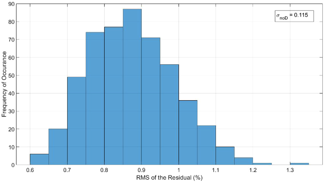
A histogram of the frequency of occurrence for RMS of the residual values for the noD monitoring period. The standard deviation of the monitoring period is labelled as ${\sigma }_{\mathrm{noD}}$ .

Although the distribution of RMS of residuals does not appear to be strictly normal, it is worth computing the standard deviations (σ) in the four datasets, and to express the increase in the mean value at each monitoring period in terms of standard deviation. This is done in Table 1, where the increase in mean is expressed in terms of σ computed in the noD monitoring period ( ${\sigma }_{\mathrm{noD}}=0.115$ ). The left column of the table shows that the standard deviation of the datasets remains fairly stable throughout the entire experiment, which is a good indication that it is the mean $\mathrm{RM}{\mathrm{S}}_{\mathrm{DN}}$ values that are increasing rather than the datasets simply becoming noisier.

Table 1.

Table of the mean $\mathrm{RM}{\mathrm{S}}_{\mathrm{DN}}$ of the residual and standard deviation for each monitoring period. The proportionate increase in the mean value of each monitoring period in terms of the standard deviation of the noD period is also displayed.

Monitoring period	Mean $\mathrm{RM}{\mathrm{S}}_{\mathrm{DN}}$ of the residual	Increase in mean $\mathrm{RM}{\mathrm{S}}_{\mathrm{DN}}$ by ${\sigma }_{\mathrm{noD}}$
noD	$0.873\pm 0.115$	$0$
6 × 3 mm	$0.926\pm 0.092$	$0.46{\sigma }_{\mathrm{noD}}$
10 × 5 mm	$1.069\pm 0.125$	$1.70{\sigma }_{\mathrm{noD}}$
14 × 7 mm	$1.823\pm 0.110$	$7.39{\sigma }_{\mathrm{noD}}$

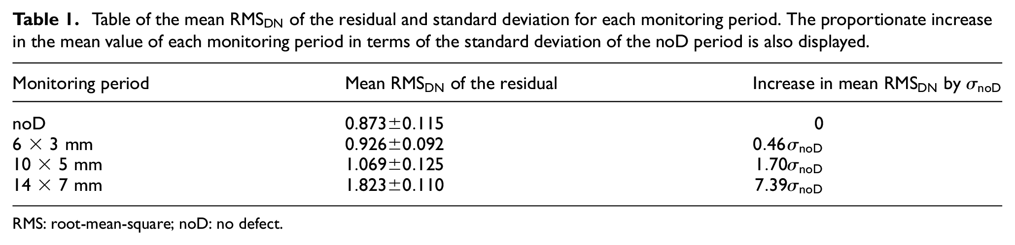
RMS: root-mean-square; noD: no defect.

If the distribution of the residuals can be approximated as normal then the number of baseline and ‘current’ readings needed to detect a given defect size is a function of the change in residual produced by the defect expressed in standard deviations. The right column of Table 1 gives the increase in mean of RMS of the residuals shown in Figure 15 in terms of ${\sigma }_{\mathrm{noD}}$ as the notch was enlarged. Two authors of this paper have recently proposed a Generalised Likelihood Ratio (GLR) method for the automated monitoring of ultrasonic signals. ⁴⁹ In that work they have shown that by limiting the number of readings to be used as input for the GLR algorithm, very good detection results can be obtained even for scenarios in which the input data does not strictly follow a normal distribution. In particular, Figure 13 of Mariani and Cawley ⁴⁹ shows that when a large number (>100) of baseline signals are available for temperature compensation, a change of mean of the monitored parameter equal to 1.5 times its standard deviation or larger can be detected with essentially 100% POD and zero false alarm rate. This suggests that the 10 × 5 mm mm defect of Figure 14 would be very reliably detected with a negligible possibility of false calls. Figure 13 of Mariani and Cawley ⁴⁹ also shows that when the signal change is approximately $0.5\sigma$ , then it is not possible to achieve a satisfactory POD value without also generating an impractically large PFA. Therefore, we can reasonably conclude that the 6 × 3 mm defect of Figure 15 would be too small to be reliably detected with the current experimental setup.

Conclusion

This paper presents a novel guided wave monitoring technique for the detection of axially-orientated cracking in piping. The guided wave monitoring system utilised circumferentially propagating SH0 waves below the cut-off of higher order modes. Circumferential SH0 waves were chosen for their good detection capabilities for axial defects and non-dispersive nature. As a test case a 6 inch, schedule 80 stainless steel pipe was chosen due to their ubiquity in industry. In each case examined the defect reflection when measured as a percentage of the incident SH0 wave proved to be too small to identify without post-processing the signals. A comprehensive FE analysis was presented to understand the behaviour of the system. For the FE analysis and experimental validation, baseline subtraction was performed on the results by comparing a model with and without a defect. Defect detection can then be performed on the resulting residual, instead of the raw signal. The residual after post-processing showed that both the defect reflection, and the decline in the incident SH0 wave after interaction with the defect can be used to detect the defect. Further analysis revealed an amplification effect that arose from the fact that the incident SH0 wave interacts with the defect on every revolution. A detection method which used the RMS of the residual signal was chosen as the preferred metric. This value was shown to increase with the size of the defect and decrease with the axial offset from the transmitter. It was established that, dependent on the defect size, axial offsets up to 3λ (130.5 mm) were feasibly detectable, giving possible coverage of 6λ (261 mm) in the axial direction in addition to the full circumference of the pipe. The experimental setup mimicked the FE setup; however, a pitch-catch system was used in the experimental validation as it reduced the initial dead-zone compared to an equivalent pulse-echo system. A notch was created in the material using EDM at an axial offset of 1.5λ (65 mm). LSTC was used to compensate for the ∼10 °C temperature swings the component experienced over the two-month monitoring experiment. A comparison with the finite element model used in previous section was performed and excellent agreement was found between the experimental results and a simulated notch of the same size, shape and position. After a statistical analysis, it was determined that a 10 mm (∼23% of the wavelength), 5 mm deep (∼45% of the wall thickness) defect offset by the experimental axial offset of 1.5λ would be detected without difficulty with a very high POD and virtually no chance of a false call.