
Abstract
One of the biggest challenges in structural health monitoring is the compensation of monitored data for environmental and operational conditions. In order to reliably estimate the changes in the structure, it is essential that the effects of environmental and operational conditions on the ultrasonic signal are compensated for before the signals are further analysed. The temperature-induced propagation speed change has the biggest effect on the ultrasonic signal and has been thoroughly investigated. This article investigates the subtler, yet also very important, changes in transducer output resulting from changes in the operating temperature. A compensation method is proposed which compensates for both the transducer phase response change and the wave’s propagation speed change. A key practical feature of the presented compensation method is that it uses only the ultrasonic signal itself for compensation estimation and can be used for any type of ultrasonic wave regardless of the type of transducer. For demonstration purposes, in this article, the results are shown for zero-order torsional guided waves, acquired by a purpose-built electromagnetic acoustic transducer. For signals with a 41.5°C temperature difference, the proposed compensation method was able to reduce the effect of environmental and operational conditions by 20 dB further (7 dB at the tail of the echo) compared to standard methods. This results in a much higher sensitivity to defects in areas where strong reflections are received. Furthermore, for the presented measurement setup, the precision to which the temperature-dependent change in wave propagation speed could be estimated was improved by 15%.
Keywords
Introduction
Guided wave ultrasound inspection is a well-established method for non-destructive testing of pipe-like structures. The guided waves can interrogate much larger areas compared to conventional ultrasound measurements. 1 While the sensitivity is lower, this enables rapid screening of structures for large defects. Measurement systems have become commercially available over the past 20 years, with national standards established.2,3 The guided wave measurements are most commonly employed in a pulse-echo arrangement, where a short signal-burst is excited, and the reflected ultrasound is recorded. This reflected ultrasonic signal is then analysed. The features and potential defects along the pipe length are identified by a trained operator.
Nowadays, permanently installed transducers are becoming more popular as improved repeatability and defect detection characteristics can be achieved when employing them in monitoring mode.4,5 In addition to the better repeatability and defect sensitivity, there are economic benefits of only gaining access once and acquiring repeated measurements without additional access costs. Access costs, such as excavation, building of scaffolding or the removal of thermal insulation can be more expensive than the inspection itself.
Ideally, any change in the ultrasonic signal refers to a change in the structure only. However, in real life, the change in environmental and operational conditions (EOCs) will also affect the recorded ultrasound signal, and the acquired signals need to be compensated first. The compensated signal can then be compared to the baseline (reference) signal, which was collected after transducer installation when the structure condition is known to be defect-free (clean).
Detailed investigations have already been conducted on the temperature-induced changes to ultrasonic wave propagation.6–8 The major effect caused by a change in temperature is an alteration of the propagation speed of ultrasonic waves: As the specimen’s elastic properties change, the ultrasonic velocity changes as well. 9 This implies that the dispersion curves for the guided wave modes change as well.10,11 While less severe, changes in the wave attenuation can also be caused by variations in the EOC. For guided waves, the variation in attenuation is strongly dependent on the coating type, therefore, a general solution is hard to find. 12
The optimal baseline selection (OBS) method was suggested to circumvent the problem of changing EOCs, where several baseline signals are acquired on a clean pipe at different temperatures and each reading is compared to the best baseline signal. 13 However, in industrial pipeline health monitoring, the structure’s temperature cannot be controlled; therefore, the OBS method may not be feasible as it is practically impossible to acquire the required number of baseline signals so that it matches the exact temperature of interest.
Even small temperature changes can result in a relatively large change in the acquired signals. It is therefore required that the results of EOCs are compensated in the ultrasonic signal. By applying a well-chosen temperature compensation method, the residual levels (difference between the baseline and the reading signal) can be decreased, meaning that smaller defects can be distinguished from the temperature variations. Furthermore, if the residual levels are lower, the structure can be diagnosed defect-free with higher confidence.
It is therefore required that the changes in the time signal caused by the temperature variations are compensated for to some extent. This is the aim of a temperature compensation method that is called baseline signal stretch (BSS). The reading signal is stretched in the best possible way before subtracting it from the baseline signal. This approach works relatively well when the temperature differences between the baseline and the reading signal are small; for larger temperature differences the signal stretch alters the wave packet shape and the baseline subtraction will not be sufficient. 4
Combined strategies of OBS and BSS have also been proposed for improved performance of temperature compensation. 14 This method uses multiple baseline signals and the reading signal is stretched to the best available baseline signal.
The problem with these compensation methods is that they compensate for the propagation speed change only, and neglect the possible effects that change the transducer output. EOC-induced changes in the transducer performance have received considerably less attention compared to the effects induced by changes in propagation speed; this is probably due to the fact that the variety of transducers that are employed all have different excitation mechanisms.
Nonetheless, some previous work that quantifies transducer performance changes and corrects for them has been carried out. Morrison et al. 15 have investigated how the lift-off of the electromagnetic acoustic transducers (EMATs) affects the arrival times of Lamb waves that they excite in plates. As a result, they have applied a correction to the extrapolated arrival time values, rather than the ultrasonic signal itself. Kim et al. 16 have applied a calibration procedure for the receiving transducer in order to obtain a conversion transfer function and to compensate for any small variations in the coupling of the receiving transducer. The calibration was performed prior to every measurement where the transducer transfer function was calculated from the transducer input current and voltage signal. Assous et al. 17 have investigated the phase-response of wideband piezoelectric transducers at different frequencies. The magnitude and phase of the transducer transfer function was measured for a wide frequency range. As a compensation the excitation signal was digitally inverse filtered. As the measured ultrasonic signal is compensated for the amplitude and phase response, the bandwidth of the transducer system is enhanced. A real-time advanced electrical filtering hardware was developed by Hurst et al. 18 for a similar purpose. An analogue second-order electrical filter is applied on the measured ultrasonic signal, which compensates for the transducer transfer function. The drawback of analogue filtering is that only causal filtering can be applied, which results in a small time delay of the signal. This compensating electrical filter did include a fine-tuning which could compensate for the temperature effects. It was observed by Labyed and Huang 19 that imaging algorithms can be corrupted due to the transducer phase response. The phase response of the transducer was evaluated from a reference glass scatterer. The imaging algorithm was modified to account for the phase response of the transducer elements. These transducer response compensation methods need calibration, or a priori knowledge about the transducer behaviour.
The work reported in the following sections investigates the combined effect of the propagation speed change and the transducer performance change (induced by temperature variations) on the ultrasound signal. An iterative compensation method is suggested, which estimates the phase and propagation speed change solely from the ultrasonic time signal. Therefore, it is believed that the proposed method is a general solution, and can be widely used for different transducers and measurement setups. The key point of the method is that separated transmitting and receiving transducers are used, so that the incident wave is recorded, and the phase information is evaluated from it. It is believed that the method could work for different types of guided waves as long as the incident wave is received and the signal is a single mode. The method is believed to be limited to cases in which reflections do not substantially overlap and do not consist of multi-modal content that propagates at different wave velocities.
It is believed that there can be further temperature changes on the ultrasonic signal in excess of the propagation speed and the transducer response, which we do not address by the proposed method. For example, the reflections may have temperature-dependent behaviour. Also, phase and group velocities of very dispersive guided wave modes may vary at different rates and, therefore, a further change is experienced on the signal.
Problems encountered by conventional temperature compensation techniques (imperfect stretch, increased residual)
Effect of temperature on ultrasonic time trace
The propagation speed change will simply result in a delayed signal arrival. Each wave packet will be delayed in relation to the propagated distance. For longer travelled distances, the arrival time change will be more significant. Figure 1(a) shows the difference between non-dispersive ultrasonic wave packets (5-cycle 27-kHz toneburst) after 3 m of propagation, when the propagation speed was 3250 and 3234 m/s, respectively. (Note that the simulated signals have propagated for some distance, and only the part of the signal where the wave packet arrives is shown.)
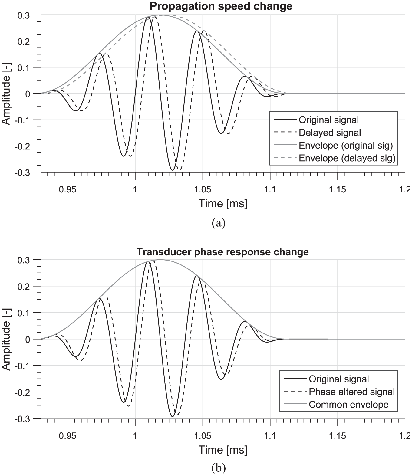
Simulated ultrasonic signals after 3 m of propagation when the excitation was a 27-kHz 5-cycle Hanning windowed toneburst. (a) Signals with different propagation speeds (3250 and 3234 m/s). (b) The effect of transducer phase response change, where the excitation phase was 0 and 35 (propagation speed was 3250 m/s for both).
It is expected that all types of transducers will change performance when their temperature is changed. The transducer’s transfer function change (phase response change) will unavoidably result in a different wave packet being excited. In the first approximation, the phase change is modelled so that the phase change is uniform across all frequencies. The uniform phase change on all frequencies will alter the carrier wave’s phase, but has no effect on the signal envelope (calculated as the Hilbert envelope), as shown in Figure 1(b). It is not genuinely true that the phase change is uniform across all frequencies; therefore, section ‘Frequency-dependent phase compensation of the ultrasound signal’ further investigates the compensation when the phase change is frequency-dependent (envelope of the wave packet is altered as well).
There are several possible reasons for the temperature-induced performance changes for bonded (either piezoelectric or magneto-strictive) transducers and EMATs:
For example, the adhesives used for bonding piezoelectric and magneto-strictive transducers can become softer at higher temperatures. Once the stiffness of the adhesive changes, it alters the resonant frequency of the transducer.9,20 Then, as the frequency response is altered, the excited ultrasonic wave will be affected by a phase change. When the piezoelectric transducer excitation frequency is close to the resonant frequency, the phase response is the most sensitive to EOCs.
EMATs are also affected by temperature. For example, the temperature changes the impedance of the EMAT (the conductivity of the coil and test specimen changes) and the excited signals will exhibit a phase change. As shown in Figure 2, the magnitude (Figure 2(a)) and the phase (Figure 2(b)) of an EMAT are affected by temperature variations. The EMAT whose construction is described in Herdovics and Cegla 21 was used for the reported measurements.
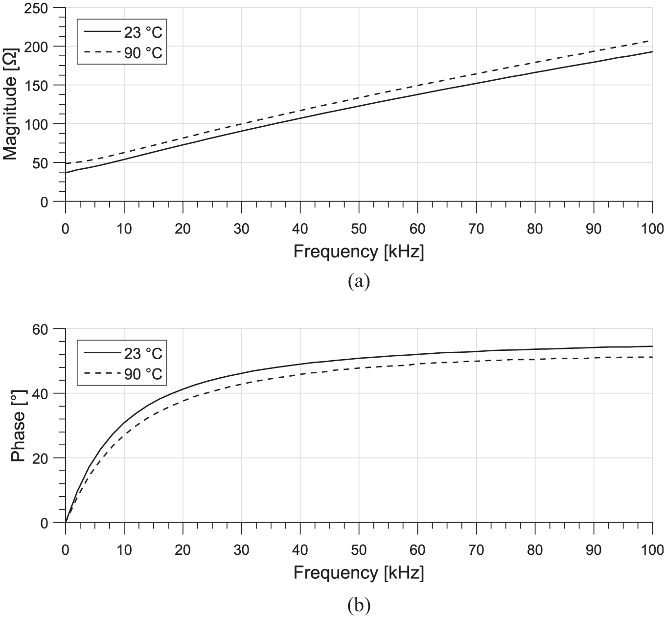
Experimentally acquired impedance for a 6-coil transmitting EMAT 21 at 23°C (solid line) and 90°C (dashed): (a) the magnitude of the impedance and (b) the phase of the impedance.
For similar reasons, additional phase changes will influence the receiving transducer performance. Furthermore, the performance of the instrumentation, for example, the signal amplifiers can be affected by temperature and can introduce further phase changes. The overall phase change that the recorded ultrasonic signal exhibits is then the addition of the phase change experienced by each part of the measurement system.
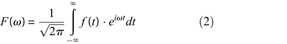
Mathematical representation of the effect of temperature changes on the signal
Let us consider a non-dispersive ultrasonic wave packet which has travelled attenuation-free in one dimension. The reference time signal recorded after
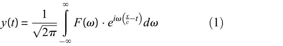
where
The temperature changes the propagation speed of the ultrasonic wave. Each wave packet will be delayed, and the delay of each ultrasonic wave packet will be proportional to the travelled distance. The time delay in the Fourier domain corresponds to the function
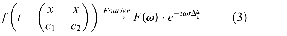
where
The effect of propagation speed change is demonstrated on simulated signals and is shown in Figure 3(a). The time signals consist of four echoes which correspond to 5, 17.5, 30 and 42.5 wavelengths of travel. In the simulation, the two signals have different propagation speeds (3250 and 3234 m/s). The difference between the two signals (shown in Figure 3(b)) is the residual error, which is increasing as a function of distance.
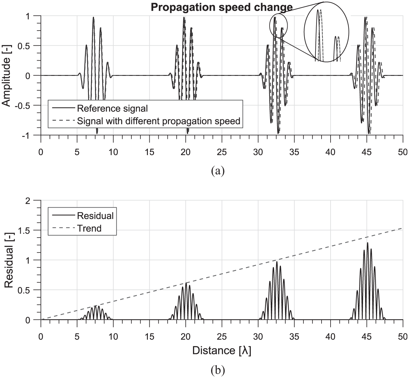
(a) Simulated ultrasonic signals with propagation speeds of 3250 and 3234 m/s and (b) their difference or residuals. An increasing trend in the residual error can be observed.
If the transducer transfer function is affected by the temperature, the excited signal will suffer a phase change (referred to as p). Usually the excitation frequency is a narrow-band pulse, so in the first instance the temperature effects will be simulated as a constant amplitude and constant phase change on the whole excitation bandwidth. The Fourier transform of the altered excited signal

The effect of excitation phase change was investigated in a separate simulation, where two signals were constructed, and the excitation phase on one signal is altered by 35° (Figure 4(a)). It was concluded that the phase change of the excitation signal has an equal effect on all echoes. The difference between the wave packets is independent of the propagation distance, as shown in Figure 4(b).
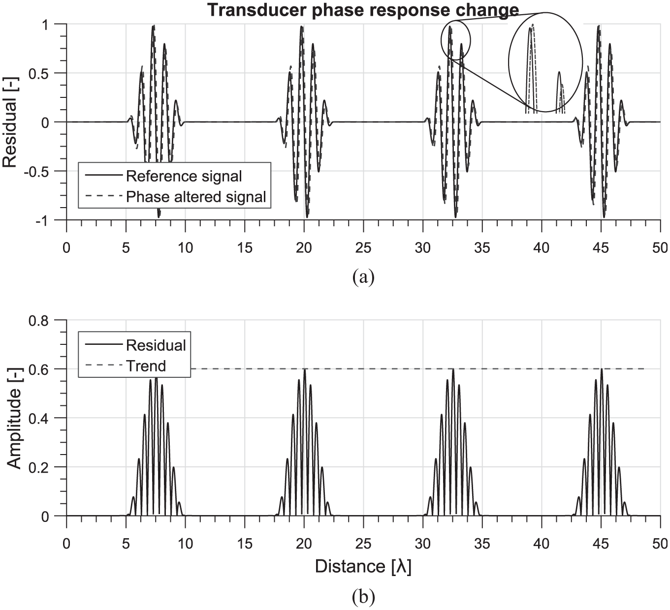
Signals with (a) different excitation phase (0° and 35°) and (b) their difference. The error observed on each wave packet is independent of the distance from the source.
The overall effect of the temperature change will be a combination of the propagation speed change and the transducer transfer function change. The time signal of the temperature altered y(t) signal is then calculated as
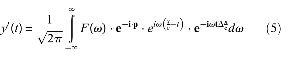
The terms by which the temperature altered signal differs from the reference signal (equation (1)) are shown in bold text. Therefore, it can be seen that the Fourier transform of the ultrasonic wave packet that is affected by propagation speed change and transducer transfer function change will be altered by the function

The phase change on each wave packet of the signal after x metre travel is
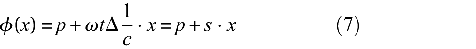
The combined phase difference
Combined effect of propagation speed change and transducer response change on the phase difference between two signals as a function of propagation distance. The phase difference due to the transducer phase response change is independent of the travelled distance, whereas the phase difference due to the propagation speed change is increasing with the travelled distance.
Imperfect single-stretch-based compensation
The conventional temperature compensation methods try to compensate the altered signal by a single stretch. The stretch estimation method searches for the optimal stretch factor in which the correlation between the baseline and the stretched reading signal is maximized. 14 Advanced algorithms were developed which are optimized with respect to computation time. 22 The work that is reported here uses these improved stretch estimation and signal stretch transformations.
If the excited signal’s phase is altered, the single-stretch-based temperature compensation methods will result in an imperfect stretch estimation. Propagation of ultrasonic wave packets (5-cycle 27-kHz toneburst excitation) were simulated, where the propagation was 6 m for all signals, but each wave was excited with a different phase. The signals are shown in Figure 6 after the optimal baseline stretch was performed on them. As the phase of the excited signal is changed, the highest correlation between the baseline and the reading is reached when the toneburst itself is mislocated (wrong signal stretch is estimated). The imperfect stretch is most notable when comparing envelopes; the envelopes of the different signals are not located in the same place on the x axis. The signals with imperfect stretch are shown in Figure 6. The error in propagation speed estimation was 12 and 23 m/s when the excitation phase was altered by 57° and 114°, respectively.
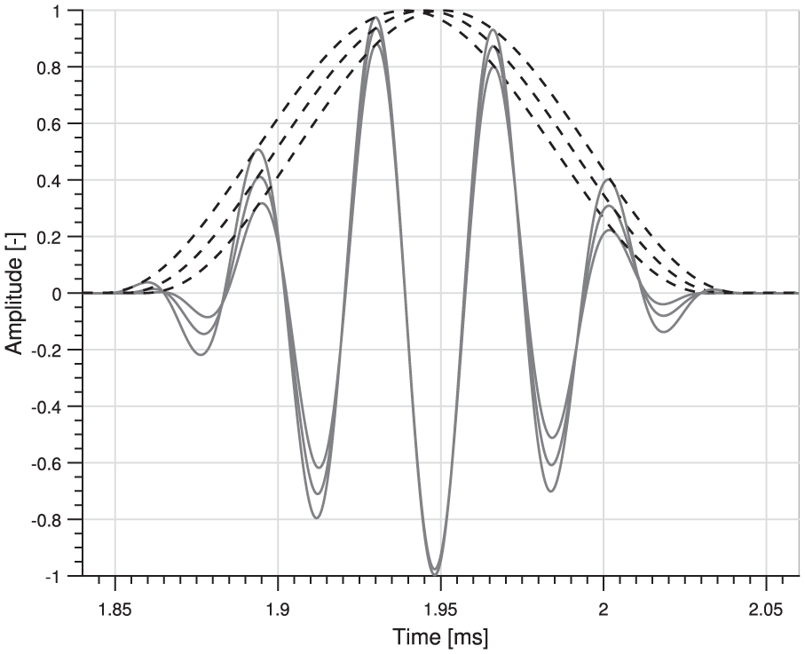
Example of ultrasound time signals with imperfect compensation on simulated signals: the correlation-based stretch estimation methods will result in imperfect stretch estimation. The propagation speed is estimated with an error of 12 and 23 m/s when the excitation phase was changed by 57° and 114°. Also, the signals do not overlap, therefore, the residual signals will be large.
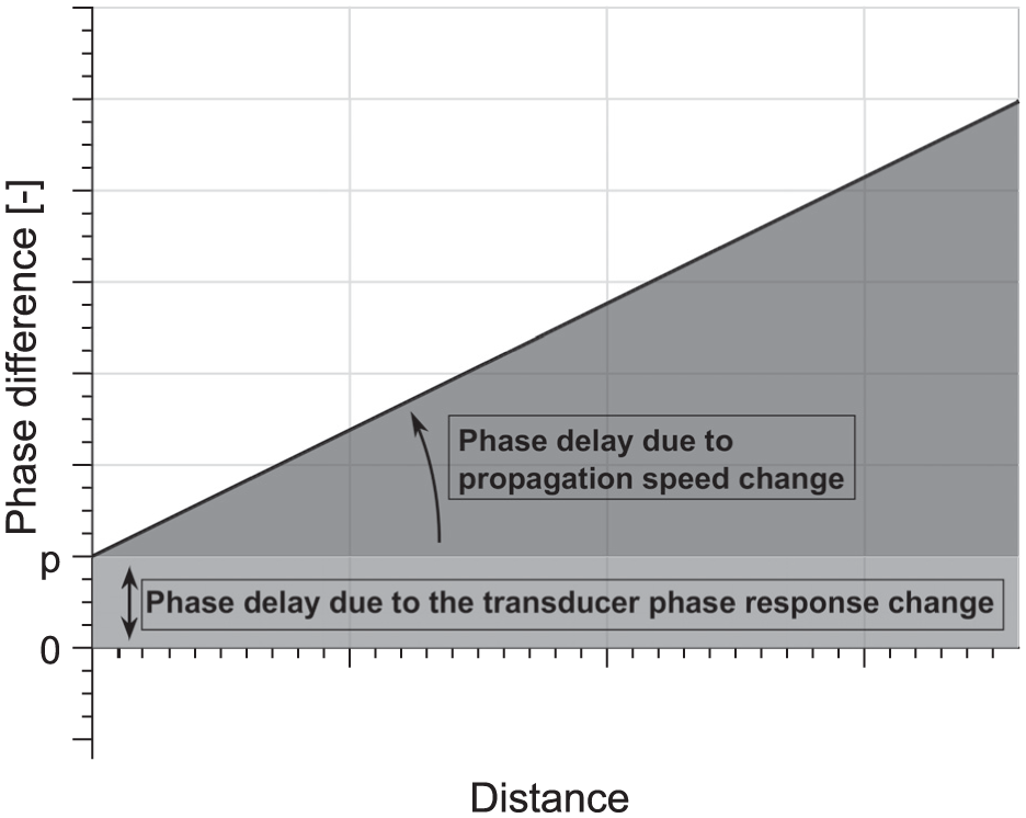
The imperfect stretch can also be explained using the phase error versus the propagated distance plots. The combined phase error (transducer and propagation speed change) caused by the temperature in function of the travelled distance is plotted with a dashed line in Figure 7. The signal stretch compensates for a linear error proportional to the travelled distance (dotted line). The remaining phase error (plotted in black) will be present in the residual signals after subtraction. It can then be observed that the estimated signal stretch (which is equal to the gradient of the slope) is different compared to the signal stretch that corresponds to the actual propagation speed change.
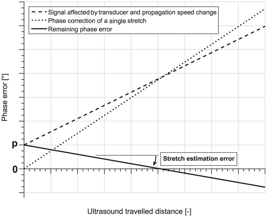
Problem with single-stretch compensation methods: the phase of the ultrasonic signal is altered according to the dashed line, whereas the signal stretch compensates for the phase error according to the dotted line. The remaining phase estimation error is represented by the black line.
If the phase change of the excitation is not compensated for on the ultrasonic time traces (for example, shown in Figure 6) the baseline and the (stretched only) reading signal will be different. At those locations of the ultrasonic signals, where larger amplitude wave packets are received (e.g. at echoes originating from features), the residual signal will increase above the noise threshold. Therefore, detecting defects is harder without excitation phase compensation.
Three different cases were investigated (shown in Figure 8) in order to estimate the severity of the uncompensated temperature effects on the residual signal: (a) the echo envelope is matched up with the baseline’s envelope, (b) the reading signal is stretched to the baseline and (c) both the phase and the propagation speed change are compensated.
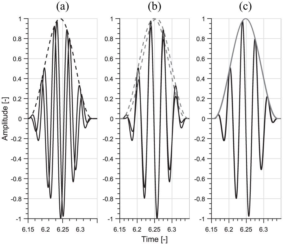
Different cases for compensation: (a) signal stretched using the envelope as the reference, (b) stretch estimated using the acquired ultrasonic signal and (c) both signal stretch and phase compensation are applied.
The residual levels are shown for each case in Figure 9. The residual levels are calculated for a 10% reflector, as this magnitude of reflection is typical of feature reflections on pipelines. It can be observed that the residual levels are the highest when the signal stretch was estimated on the envelope of the signal (case (a)). Note that in case (a), despite the stretch being estimated from the envelope of the signal, the residual is calculated by subtracting the signal itself, not the envelope. If the signal stretch is estimated on the ultrasound signal itself, the residual levels are lower (case (b)). However, in this way an imperfect stretch estimate is made, as previously discussed.
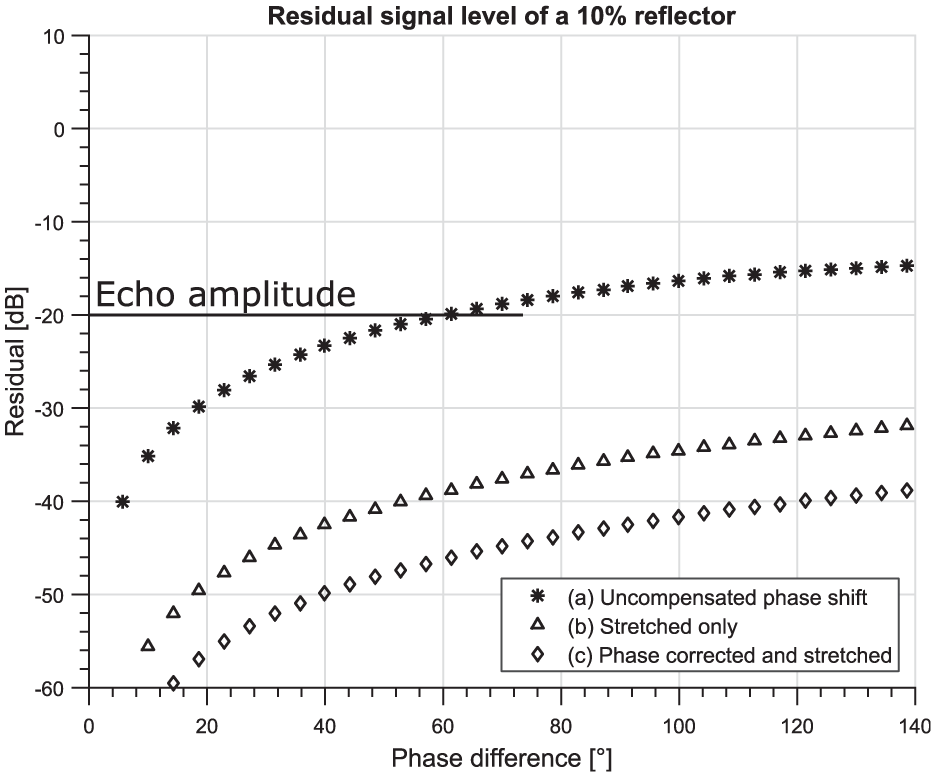
Residual error after baseline subtraction associated with different methods (shown in Figure 8) on a logarithmic scale. The error was calculated for a 10% reflector.
The lowest residual levels are reached (therefore, the most favourable case is) when the phase change is recovered, and the propagation speed change is compensated by a signal stretch (case (c)). The remaining error in this case is the distortion in the signal shape due to the signal stretching. 14 Figure 9 shows that the decrease in the residual when comparing cases (b) and (c) is around 7.3 dB, but this depends on how severe the transducer phase change is as a result of temperature change. In the simulation, it was assumed that the temperature change results both in a phase change of 1° and a 0.66 m/s reduction in propagation speed.
Proposed, improved, practical compensation technique
Compensation method
For presentation purposes, the compensation concept and the results in this article are shown on torsional guided wave signals acquired by an EMAT transducer. The torsional guided wave signals were acquired on a 5-m-long 3-inch NPS mild steel pipe using electromagnetic acoustic transducers. The EMAT transducer was previously developed by the authors, as an alternative to be bonded on sensors with the aim of achieving better long-term signal stability. However, it is still affected by temperature variations, which must be compensated for. 21 As shown in Figure 10, two transmitter transducers are used for the measurements so that directional control can be achieved. The receiving transducer is placed 40 cm from the transmitting transducers. The effect of the axial separation is that the incident (direct) wave is separated from the cross-talk signal (the cross-talk being the transmitted signal electromagnetically coupled to the receiver transducer). In conventional EMATs, the cross-talk is magnitudes higher than the ultrasound signal itself, and would prevent receiving the ultrasound signal for a significant time; a special cross-talk reduction hardware system was developed by the authors. 23 This allows us to suppress the cross-talk to the minimal level and receive the incident wave in the ultrasound signal, as shown in Figure 11.
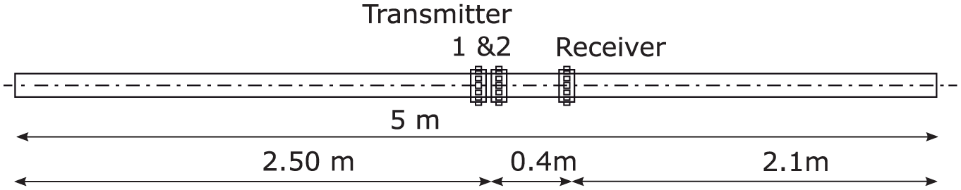
Measurement setup for acquiring signals on a 5-m-long 3-inch NPS pipe using two transmitting and one receiving transducer.
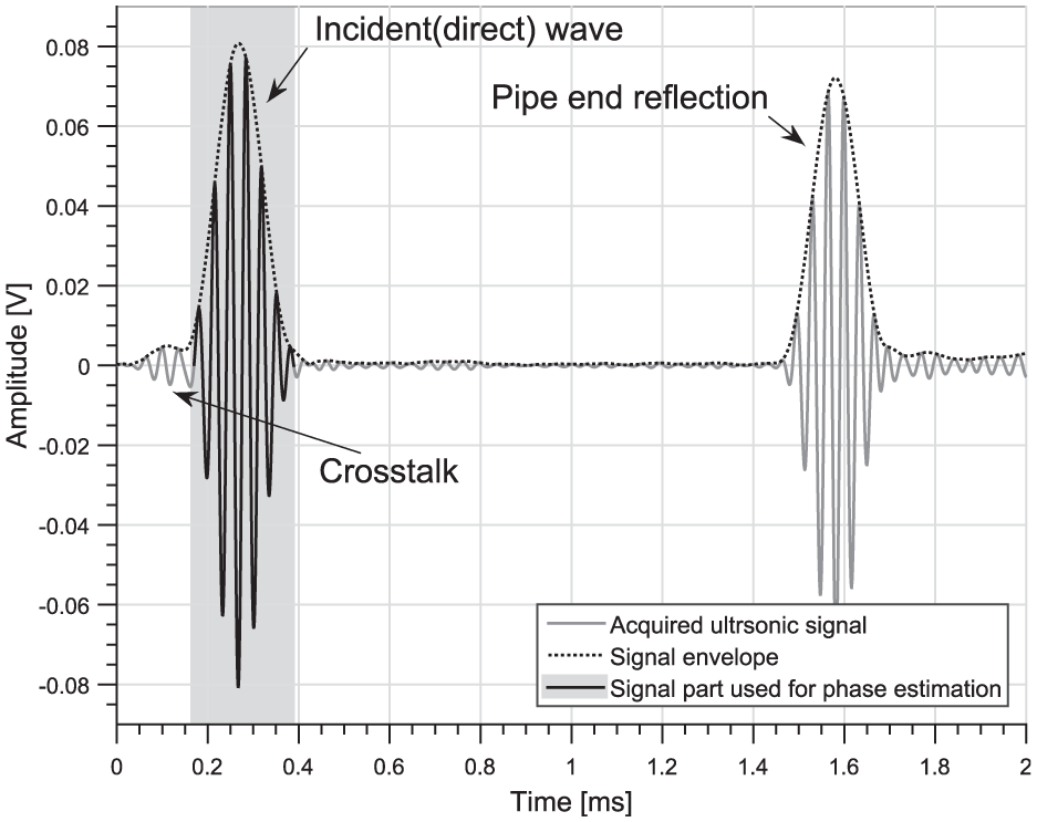
Acquired right travelling torsional guided wave travelling on the 3-inch test pipe. The incident wave packet of the signal is used for phase change estimation and is highlighted in black on a grey background.
It is possible to estimate both transducer phase response change and propagation speed change if two wave packets are present in the ultrasonic time signal. In our case the two wave packets will be the incident wave (shown in black in Figure 11) and reflections from the pipe features (end reflection in our case).
Later echo signals (e.g. the pipe end reflection in our example) are mainly affected by the arrival time change, as the propagation distance is significantly larger. However, as the incident wave has travelled for a small distance only, it is mainly affected by the transducer performance changes. Although the transducer change is the major effect on the incident wave, the propagation speed change also has a slight effect on the incident wave. Therefore, a one-step compensation is challenging to develop. Instead, an iterative method is suggested, which performs signal stretch and phase compensation multiple times.
The idea behind the iterative method is that once a good propagation speed change estimate exists (and is corrected for), a more precise phase change can be estimated. Also, once a good estimate of the phase correction is available, a more precise stretch estimate can be made.
Therefore, in the first step an initial propagation speed change is estimated, and the phase change is estimated after the propagation speed change is corrected for. In the next step, a more precise propagation speed change is estimated on the phase compensated signal. When the phase is estimated on an early arrival and the stretch on a later echo (as shown in Figure 11), the estimated values converge rapidly. The whole iterative phase compensation method is also presented on a flow chart in Figure 12.
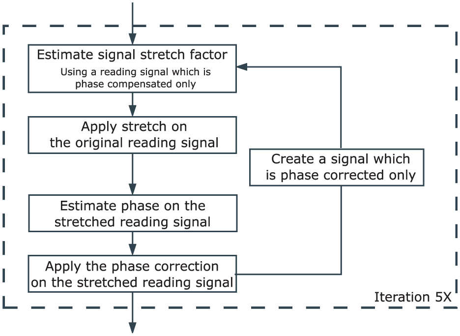
Flow chart of the iterative temperature compensation method: the signal stretch is estimated on a signal which is phase compensated only (in the first iteration the signal is simply the original reading signal). Then the stretch factor is applied on the original reading signal. Then the phase difference is estimated between the baseline and the reading signal, and is applied to the stretched signal. This iteration is repeated five times, as after this number of iterations the stretch and phase estimates only change negligibly.
Frequency-dependent phase compensation of the ultrasound signal
In the previous sections, it was assumed that the phase change caused by the temperature change is equal and uniform across all frequencies, and the signal envelope of the excited signal does not change. Unfortunately, this is not necessarily true. The phase change of the transducer might be frequency dependent, therefore, not only the phase of the carrier wave, but the shape of the envelope changes as well. This means that the Fourier transform of the altered packet will be

where
In order to calculate the frequency-dependent phase correction, the Fourier transform is calculated for both the baseline signal’s incident wave and the reading signal’s incident wave. A filter is then applied on the signal spectra so that only the main lobe is used for further calculations (19–37.5 kHz). The ratio between the two calculated complex Fourier spectra is the frequency-dependent amplitude and phase correction. The phase correction is then applied on the Fourier transform of the whole reading signal, and the inverse Fourier transformation is the phase compensated reading signal.
An example of the frequency-dependent magnitude and phase correction is shown in Figure 13 when the baseline was acquired at room temperature, and the reading was acquired on a 64.5°C pipe.
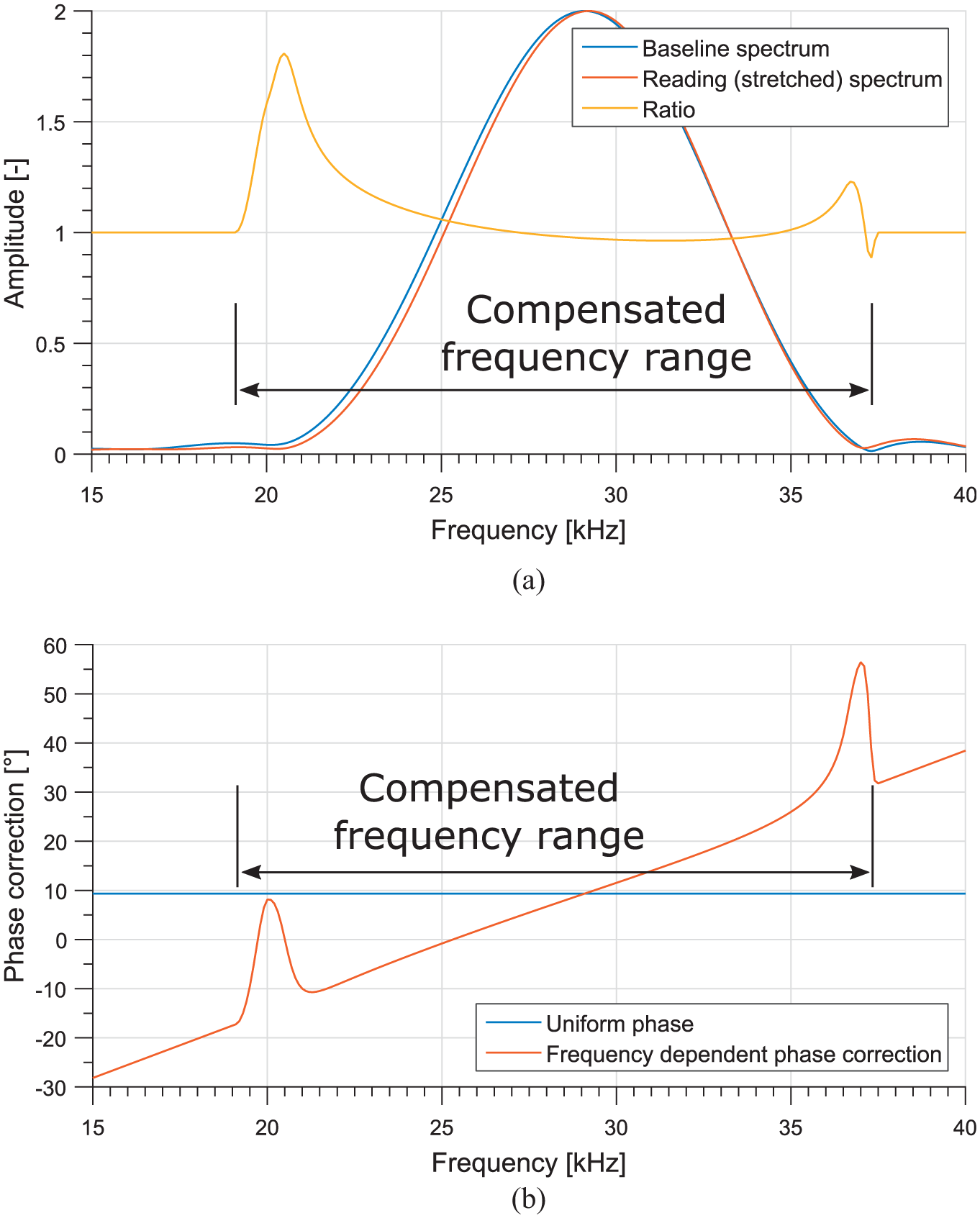
The Fourier magnitude spectrum of the baseline’s and the stretched reading signal’s incident wave packet is slightly different due to the performed stretch (a). The frequency-dependent correction corrects for its unwanted effect (frequency noise) by applying a (a) magnitude and (b) phase correction on the ultrasonic signal. The compensated frequency range is selected as the main bandwith of the excitation signal spectra (19–37.5 kHz in this example). The estimated uniform phase is shown for reference.
It is important to note that by performing the frequency-dependent phase correction, an additional benefit is implemented: the signal stretch performed on the ultrasonic signal alters the frequency content of the wave packets (see Figure 13(a)), and it will result in the so-called frequency noise. 24 This frequency noise will be removed when the frequency-dependent phase correction is applied to the ultrasonic signal.
Experimental results
Signal acquisition setup
A 5-m-long finned electric heater element was placed inside the pipe so that signals can be acquired when the pipe temperature is fluctuating. The heater temperature was measured with thermocouples, and was also controlled so that the desired pipe temperature can be set. The whole pipe was fitted with insulation, so a uniform temperature distribution is reached within the pipe. The temperature distribution along the pipe was measured with several thermocouples. The heating setup is shown in Figure 14.
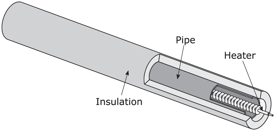
Measurement setup for acquiring signals with arbitrary pipe temperature. Finned heater element is used for heating, while the pipe outer surface is well insulated from the environment.
Before starting the measurements, the pipe was heated up, then the heater temperature was kept constant while the temperature distribution inside the pipe became uniform. Once the heating was turned off, the signals were repeatedly acquired while the temperature dropped to room temperature. Roughly, one measurement per degree Celsius in temperature change was measured. The pipe cooling down process is fairly long (∼3 h time constant), and a signal acquisition with 50 averages takes less than 30 s. Therefore, changes in the pipe temperature while acquiring a signal are negligible.
Compensation of acquired ultrasonic signals generated by EMATs
The phase compensation method was tested on acquired torsional guided wave signals. The baseline signal is shown in Figure 11, where the incident wave is highlighted. In the first iteration of the compensation method the propagation speed is estimated on the echoes. The arrival time difference of the ultrasound echoes (and incident wave) is compensated by signal stretch. As the arrival time of the echoes are compensated by the signal stretch, the remaining difference is due to the different transducer performance. Then, the phase difference between the baseline and the stretched reading is estimated, and the reading signal is compensated. Example signals are shown in Figure 15 when the baseline was acquired on a room temperature pipe (23°C), and the reading signal was acquired on a pipe at 64.5°C. The baseline signal is plotted in black, the stretched reading signal with a dotted line, and the reading signal which is stretched and phase corrected is plotted in grey. It can be observed that the signal that is stretched and phase compensated and the baseline resemble each other much more closely than the baseline and the signal that is only stretched.
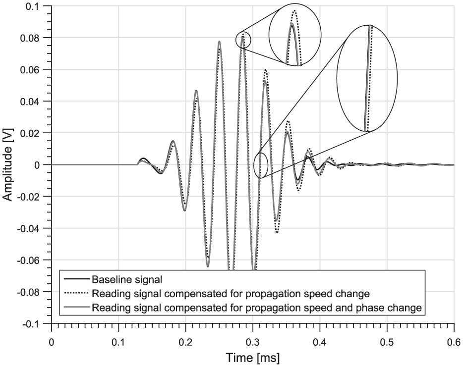
The incident wave of the ultrasonic signals: baseline signal (black), reading signal compensated for propagation speed (dashed) and phase and propagation speed change compensated (grey). The temperature difference between the baseline and the reading was 41.5°C.
In the next iterations the propagation speed change is re-estimated using the phase compensated reading signal. This will result in a more accurate propagation speed estimate. Then, after re-calculating the stretch factor and the stretched reading signal, a more accurate phase estimation can be produced. The iteration steps can be repeated until the desired precision is reached. It was observed that in our measurement setup the estimated values are exponentially converging to the final value. For example, for an iterative compensation where the propagation speed difference between the signals was 26 m/s (50°C temperature difference), the estimate converged to within 0.03 m/s of the final result within three steps.
It is important to note that a stretch performed on the ultrasonic signal distorts the shape of the wave packet (squeezing or expanding the wave packets). After subtraction, this results in small residual signals. This is often called the ‘frequency noise’, as the stretching of the wave packet slightly alters the frequency content of the signal. It is possible to compensate for the wave packet shape distortion with the ratio of the original and stretched wave packet’s spectra.24,25 If the iterative temperature compensation method uses frequency-dependent phase difference estimation between the baseline and the (stretched) reading signal, the frequency-dependent phase correction will automatically correct for the frequency noise as well.
Residual signals
The improvement of the proposed compensation method can be demonstrated on the residual signals. Figure 16 shows the calculated residual signals when only the propagation speed is compensated (shown in grey), and when the phase response change is compensated as well (black). As expected, the residual is highly improved at the echo location, and the residual is not sacrificed at the coherent noise part of the signal.
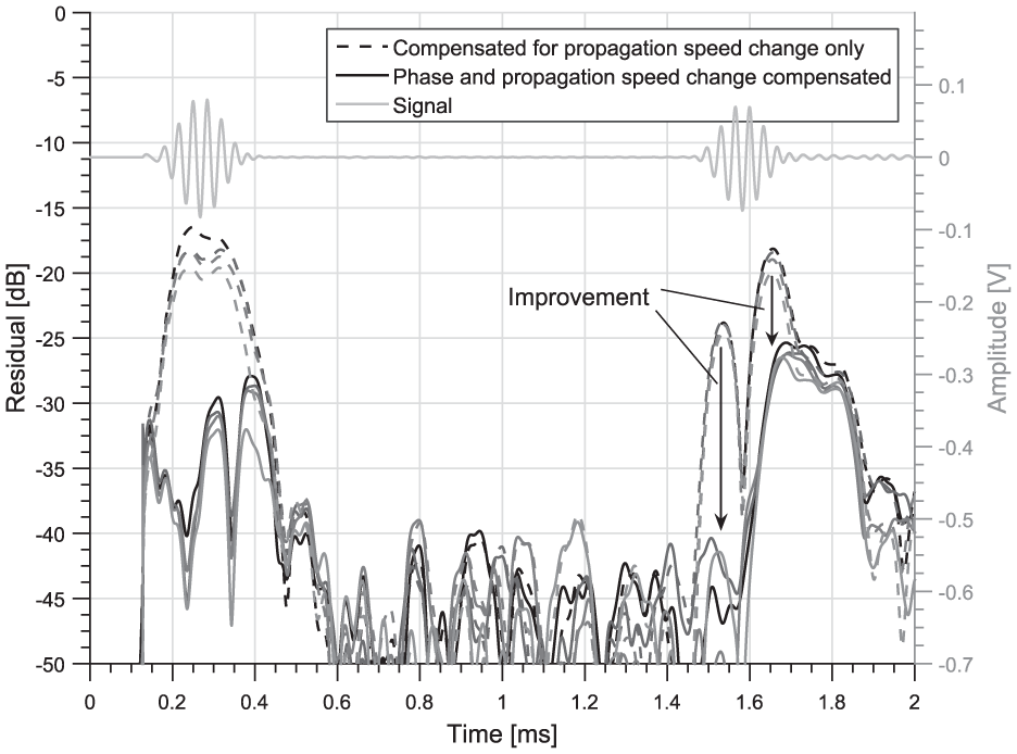
Calculated residual signals when the temperature difference between the baseline and the reading signal was 41.5°C. The residual is calculated when the reading signal was compensated for the propagation speed only (dashed), and when it was also phase compensated (solid). For demonstration purposes, for each compensation strategy four signals are shown on a different greyscale. These signals were acquired at a different time during the thermal cycling.
20 dB improvement was achieved at the echo location (1.5–1.7 ms) compared to the conventional signal processing techniques, when the temperature difference of the pipe during the acquisition was 41.5°C. However, at regions where coherent noise is temperature dependent (such as tail of echo), only 7 dB improvement was reached. The reason for the modest improvement at the tail of the echo (1.7–1.9 ms) is currently under assessment. One possible reason is that the tail of the echoes are temperature dependent (further to the transducer-induced changes). Another possible reason is that the direction control may not be perfect, as the echo coming from the other direction (arriving roughly at 1.8 ms) is not perfectly processed in the directional control algorithm. Further evaluation will be carried out in the near future on a new measurement setup (we do not want to disturb the current setup, as it is being used for evaluating long-term stability of the system).
The improved residual levels result in a much higher sensitivity (up to 7 times) for small defects at the feature reflections.
The compensation method was tested while several temperature cycles were performed on the system. The signals were collected during every cycle and on roughly every degree Celsius temperature change. Further results were selected from the large acquired data set. Figure 17 shows the residual signals for the conventional algorithm (dashed) and the proposed phase compensation algorithm (solid) for (a) 15°C and (b) 30°C temperature difference. Obviously, for lower temperature differences fewer temperature effects are to be removed, therefore, the phase compensation has a lower effect. This also implies that for large temperature differences the phase compensation method will have an even larger effect, and could be essential for monitoring applications.
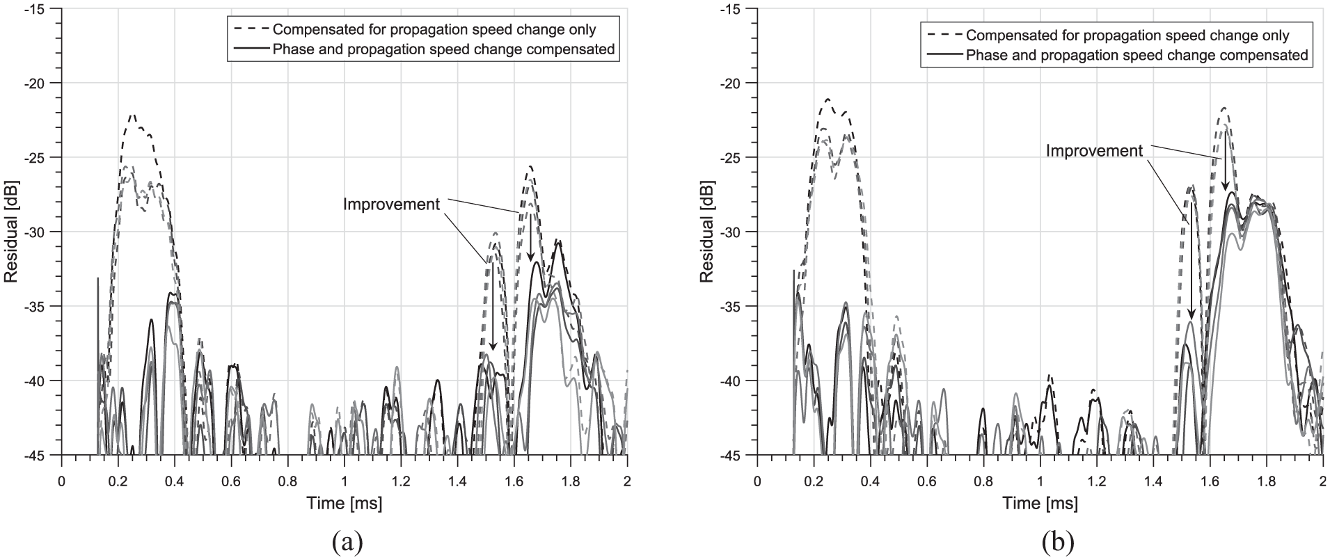
Residual signals plotted for conventional signal stretch (dashed), and when the hereby presented temperature compensation algorithm was applied (solid). The residual signals and the improvement of the proposed compensation method is shown when the temperature between the baseline and the reading signals was (a) 15°C and (b) 30°C. Four signals (shown on a different greyscale) were selected from different temperature cycles to demonstrate the robustness of the technique on different signals.
Improved stretch factor estimation
A large number of reading signals were acquired when the pipe temperature was varied from room temperature up to 73°C. The propagation speed was estimated for each reading signal. Figure 18 shows the estimated propagation speed as a function of the pipe temperature for each iteration step. The estimated stretch factor is already close to the final estimate after the second iteration step. It is thought that the number of iterations that is needed for a good estimate depends on the echo location. In the case when the source of the echo (reflector) that is used for propagation speed estimation is far enough (>2–3 m) from the receiving transducer, the convergence is quick.
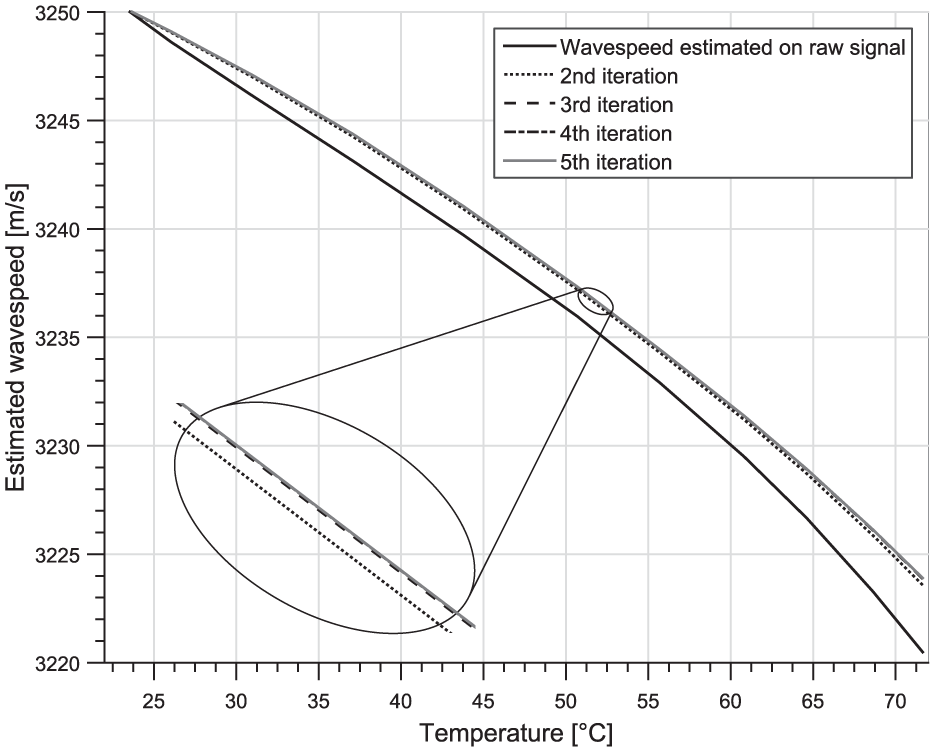
Estimated wavespeed as a function of the pipe temperature for each step in the iterative compensation method. The estimated wavespeed quickly converges to the final value.
Results when defect reflection is present in the acquired reading signal
The iterative phase compensation method was tested when a small defect reflection is present in the acquired reading signal. A synthetic reading signal was created, where a simulated defect reflection is superposed onto the experimentally acquired signal. The use of synthetic data sets is common for damage detection investigations.26–28 The defect reflection is simulated to be 20 cm from the pipe end, therefore, the defect reflection is expected to be around 1.45 ms, which overlaps with the pipe end reflection. The simulated amplitude for the defect reflection is 3% compared to the pipe end reflection.
Both the conventional stretch based and the proposed iterative (stretched and phase compensated) temperature compensation methods were applied onto the reading signal and the residual signals are plotted in Figure 19. For reference purposes, the residual is plotted with dashed lines when no defect is present in the reading signal. Also, the baseline signal is shown in grey so that the timing is better understood.
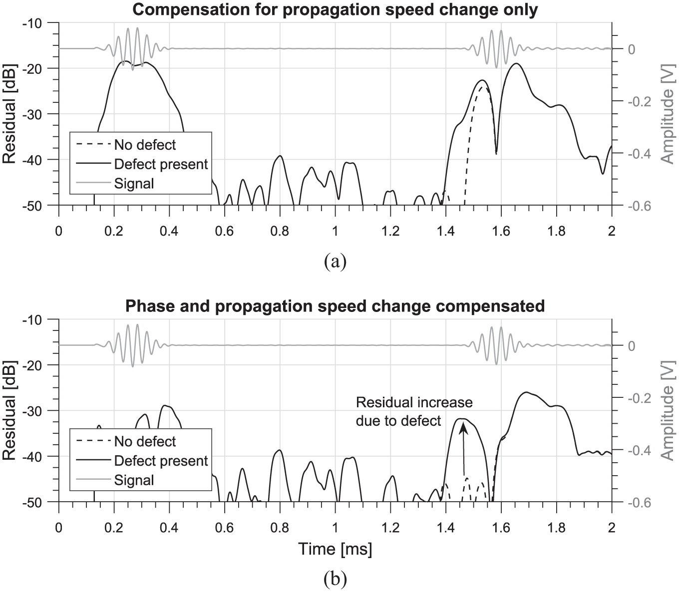
Residual signals using synthetic reading signal (a 3% defect reflection is simulated 20 cm away from the pipe end reflection and is added to the acquired measurement data). (a) Adding a defect to the reading signal has only a small effect on the residual levels for convention stretch-based temperature compensation, however, (b) the presence of the defect significantly increase the residual levels when the the proposed iterative compensation method is used. The temperature difference between the baseline and the reading signal was 41.5°C.
The residuals for the conventional stretch-based temperature compensation are plotted in Figure 19(a), where the presence of the defect reflection does not increase the residual level significantly (at 1.45 ms). In contrast, Figure 19(b) shows the residual signals when the iterative temperature compensation method was applied. When the defect reflection is present in the reading signal, the residual (at 1.45 ms) is significantly larger compared to the defect-free option.
This implies that by compensating for the transducer phase response changes the residual levels are decreased, and the defect reflection is easier to identify from the residual signals.
In the residual signal from 1.65 to 1.85 ms the noise is relatively large as the pipe end reflection is a 100% reflector. It is expected that most features in pipelines (e.g. welds) will have a reflection coefficient ∼10%, so that the noise in those residuals are expected to be lower as well.
Discussion
Uneven pipe temperature
As discussed in the previous section, the conventional temperature compensation methods will result in an imperfect stretch estimate. The problem with this is that if more features are present in the pipe, the arrival time difference of some echoes will be compensated imperfectly. This will result in an increased residual signal, due to the baseline and reading being out of phase at feature locations.
The newly proposed method has the advantage of estimating a more precise stretch factor. The benefit of the precise stretch factor estimation is legitimate only if the pipe temperature is fairly uniform along the whole pipe. It is possible for large structures to have a temperature gradient along the axis, for example, if insulation is missing, or a part of the pipe is buried. In case the pipe segments are at different temperatures, it is suggested that multiple stretch factors are applied to different pipe segments. 29 Should multiple stretch factors be required for the compensation, the importance of a precise stretch estimate is reduced. However, the improvement of the phase compensation will still be beneficial, as the defect monitoring capability will be improved at the feature locations by the reduced residual levels.
Transducer ageing
It is possible that the transducer performance changes over time. For example, the degradation of bonded piezoelectric transducers was investigated by researchers, 30 and it was concluded that amplitude and phase changes may result when the adhesives are affected by cyclic thermal loading. In case the reading signal is collected on a degraded transducer (assuming the signal strength is still adequate), the phase compensation method would be able to detect and correct for the phase changes caused by the degradation. The severity of the degradation could then be monitored from the phase difference estimates.
A similar concept was developed by Mulligan et al. 31 for correcting the ultrasonic signals in imaging applications. The phase difference caused by the degradation was estimated from electrical admittance curves, rather than from a reference part of the signal.
Conclusion
In this article, we propose a novel temperature compensation method for both the transducer phase response change and the propagation speed change of the ultrasound. The incident wave (first signal arrival) is mainly affected by the transducer phase response change, as the effect of the propagation speed change is small due to the small separation distance between the transmitting and receiving transducer.
An iterative compensation method is suggested, which uses the incident wave for phase change estimation, and the rest of the ultrasonic signal (echoes) for propagation speed change estimation. The excitation phase difference and propagation speed difference is compensated after each step, and a more precise estimation can be performed after each step. The estimate values converge to their final value quickly, and the convergence region of 0.1% is reached within three steps.
The methodology can also be applied when the transducer phase response change is frequency dependent. The improvement of the proposed compensation method compared to the single-stretch-based methods is demonstrated on the residual signals. 20 dB improvement was achieved at the echo location compared to the conventional signal processing techniques, when the temperature difference of the pipe during the acquisition was 41.5°C. However, at regions where coherent noise is temperature dependent (such as tail of echo), only 7 dB improvement was reached. The decrease in the residual signal means that the effects of the temperature change are better compensated; therefore, smaller defects can be identified near the reflectors.
Footnotes
Declaration of conflicting interests
The author(s) declared no potential conflicts of interest with respect to the research, authorship and/or publication of this article.
Funding
The author(s) disclosed receipt of the following financial support for the research, authorship and/or publication of this article: Both authors would like to thank the EPSRC for funding under the Grant EP/K033565/1.