Sage Journals: Discover world-class research

Abstract

Ageing stock and extreme weather events pose a threat to the safety of infrastructure networks. In most countries, funding allocated to infrastructure management is insufficient to perform systematic inspections over large transport networks. As a result, early signs of distress can develop unnoticed, potentially leading to catastrophic structural failures. Over the past 20 years, a wealth of literature has demonstrated the capability of satellite-based Synthetic Aperture Radar Interferometry (InSAR) to accurately detect surface deformations of different types of assets. Thanks to the high accuracy and spatial density of measurements, and a short revisit time, space-borne remote-sensing techniques have the potential to provide a cost-effective and near real-time monitoring tool. Whilst InSAR techniques offer an effective approach for structural health monitoring, they also provide a large amount of data. For civil engineering procedures, these need to be analysed in combination with large infrastructure inventories. Over a regional scale, the manual extraction of InSAR-derived displacements from individual assets is extremely time-consuming and an automated integration of the two datasets is essential to effectively assess infrastructure systems. This paper presents a new methodology based on the fully automated integration of InSAR-based measurements and Geographic Information System-infrastructure inventories to detect potential warnings over extensive transport networks. A Sentinel dataset from 2016 to 2019 is used to analyse the Los Angeles highway and freeway network, while the Italian motorway network is evaluated by using open access ERS/Envisat datasets between 1992 and 2010, COSMO-SkyMed datasets between 2008 and 2014 and Sentinel datasets between 2014 and 2020. To demonstrate the flexibility of the proposed methodology to different SAR sensors and infrastructure classes, the analysis of bridges and viaducts in the two test areas is also performed. The outcomes highlight the potential of the proposed methodology to be integrated into structural health monitoring systems and improve current procedures for transport network management.

Keywords

critical infrastructure transport networks infrastructure resilience early warning roadway bridges MT-InSAR remote sensing Los Angeles Italy

Introduction

Civil infrastructure networks supply our basic needs for mobility, power, water and communications, playing a central role in the growth and development of national economies. However, the structural failures of the last 30 years reflect the vulnerability of existing infrastructure,^1,2 and western countries are facing growing pressures to upgrade their national infrastructure systems.³ Bridge collapses, water main breaks, gas pipe ruptures, dam failures and steam pipe explosions are some examples of infrastructure failures.

Evidence has shown that most of these failures are related to ageing stock.^4,5 In many countries, pipelines, roads, railways and bridges are reaching the end of their life service and need to be upgraded.^6–9 Infrastructure maintenance requires large amounts of investment. The American Society of Civil Engineers⁷ found that US infrastructure was in an overall ‘poor condition’ and would require an investment of $2.2 trillion to fix. Germany’s Federal Ministry of Transport¹⁰ has launched a €270 billion-investment programme focused on the national transport infrastructure over the next 15 years: 70% of the budget is allocated for structural maintenance and repair of existing facilities. In Italy, the Ministry of Infrastructure and Transport has approved an additional €28 billion of rail and road investment for the 2019–2023 phase.¹¹ The UK’s National Infrastructure Plan¹² allocated over £88 billion toward the transport segment, and £6.7 billion are required to upgrade substandard bridges.

The vulnerability of transport infrastructure is traditionally assessed through field surveys and site-based instrumentation, such as tilt sensors and crack gauges.^13,14 The larger the transport network, the higher the maintenance costs are, making it impractical to conduct all the necessary point-based measurements. Due to the high cost of sensors, only a few assets around the world are equipped with site-based instruments, while the health-structural evaluation is mainly performed through visual inspections.^15–18 Inspection timelines are different for different countries and specific assets. For example, in the USA routine bridge-inspections are usually performed every 1 or 2 years, while underwater inspections take place every 6 years.¹⁹ In Germany and the UK, bridges are surveyed once every 3 years and receive a full-check every 6 years. French bridges receive a general inspection every year and a detailed inspection every 3 years.^20,21 In the Netherlands, bridges are inspected every 6 years.²² The low frequency of these investigations and the variable methodology and accuracy of these evaluation techniques¹³ mean that transport infrastructure often lacks systematic and reliable structural inspections.

A promising solution to this problem is offered by the exploitation of space-borne Interferometric Synthetic Aperture Radar (InSAR) to monitor civil infrastructure on a large scale. InSAR-based monitoring can be performed at faster rates compared to traditional monitoring, allowing savings of time and resources. In particular, Multi Temporal InSAR (MT-InSAR) techniques^23–25 allow the extraction of surface displacements over time from high-resolution SAR images – that is, up to 2–5 m for SAR satellites operating at C-band (∼5.6 cm wavelength) and about 1 m for X-band (∼3 cm wavelength) SAR sensors.²⁶ MT-InSAR techniques enable weekly detection of surface deformations with a precision of up to the millimetre scale.^27,28 These techniques are based on the identification of point-targets showing stable scattering properties along a time-series of InSAR images. Due to their physical properties, buildings, steel rails, bridges and dams can satisfactorily generate Permanent (or Persistent) Scatterers (PSs), that is, point elements providing a temporally coherent electromagnetic backscattering. This makes MT-InSAR techniques an excellent tool for detecting deformations over built-up areas^29–31 and civil infrastructure.^{15,18,32–34}

Recent studies have shown the feasibility of space-borne MT-InSAR techniques to provide accurate spatial information for building monitoring,^35–44 bridges,^16,45,46 dams,^47–50 railways^51–54 and other linear infrastructure,^55–59 demonstrating that remote-sensing data can be effectively utilised in combination with conventional ground-based monitoring systems, such as precise levellings and automated total stations. However, the information obtained from MT-InSAR analysis typically consists of a huge amount of data. For civil engineering applications, these data need to be related to specific buildings and infrastructure. The manual identification of anomalies on surface features allows accurate results, but it is costly, time-consuming and requires expertise to process and analyse, limiting the timely dissemination of information provided by MT-InSAR techniques.

Geographic Information Systems (GIS) facilitate the integrated analysis of large volumes of multi-disciplinary data, allowing the integration of remote-sensing measurements and civil engineering assessment procedures.^{16,39,57,60–63} To facilitate a preliminary identification of the most vulnerable infrastructure assets or critical locations along linear infrastructure systems, a methodology based on the fully automated integration of MT-InSAR data and a GIS-based analysis is presented in this paper. The proposed methodology automatically processes large volumes of PS displacement time-series and road network databases to extract deformation data over a given network, and performs local deformation analysis designed to detect anomalous differential movements between parts of the same piece of infrastructure. Differently from existing detection methods,^58,61–64 the methodology presented in this paper is designed to analyse InSAR displacements belonging to infrastructure only, and it is independent from the source of movement causing the deformation. Results are used to generate a report displaying the location of identified anomalies along the roads, as well as an indication of the quality of the monitoring in terms of number of PSs available for each infrastructure. As the detected anomalies might indicate precursory signs of structural distress, the proposed methodology can be used to target further investigations and detailed structural analysis for informed operations and maintenance planning. The developed algorithm was applied to the Los Angeles highway and freeway network and the Italian motorway network, to demonstrate its practical capabilities. Then, the proposed methodology was used to evaluate bridges and viaducts in Los Angeles, California, USA, showing its flexibility to the analysis of different infrastructure types. Finally, the case of an Italian motorway viaduct that was damaged in 2015 is presented and analysed in relation to the outputs of the developed algorithm to determine whether the proposed methodology could be used to guide further investigations.

Literature review

Multi-Temporal InSAR (MT-InSAR) techniques have proven effective in mapping surface displacements.^65,66 Unlike the traditional Differential Interferometric SAR (DInSAR), which is based on a two-image configuration, these techniques exploit multiple SAR images over the same area to reconstruct the temporal and spatial evolution of surface deformations⁶⁷ with a high level of accuracy.

Since the late 1990s, a diverse range of stacking techniques were developed to retrieve surface deformations from large numbers of SAR images. Permanent (or Persistent) Scatterer (PS) Interferometry^24,25 was established to overcome the limitations of conventional InSAR – that is, geometric decorrelation and atmospheric effects – and provide a full resolution scatter analysis without including multi-looking operations, such as the SBAS techniques.^68,69 PS Interferometry (PSI) is a multi-image approach that is based on the identification of coherent radar reflectors, that is, permanent scatterers (PSs), over a sequence of interferograms in a certain area, allowing the reconstruction of the temporal and spatial evolution of superficial deformations affecting the ground and structures. This MT-InSAR technique can achieve a millimetre-scale accuracy on a time-series of surface displacement measurements.^27,28,70

Since 2007, the second generation of space-borne SAR missions,^71–73 for example, TerraSAR-X (TSX), COSMO-SkyMed (CSK) and Sentinel-1A/B (SNT), has provided a spatial resolution in the order of metres and a temporal resolution of a few days.²⁶ Thanks to these developments, the density of PSs extracted from high-resolution SAR data is up to 6 times higher than from medium-resolution SAR, for example, RADARSAT-1 and Envisat.⁷⁴ The combination of high spatial density, wide coverage and high sensitivity to small deformations has enabled the study of the deformation of individual assets on a large scale, increasing significantly the potential of MT-InSAR techniques.⁷⁵

The physical nature of PSs makes MT-InSAR techniques extremely effective for monitoring urban areas. PSs are point elements which backscatter the signal emitted by a space-borne SAR sensor. Thanks to their geometric configuration and dielectric properties,⁷⁶ PSs can remain stable within the stack of processed images. Investigations on the response of built-up areas to microwave radiation from satellite SAR systems led to the identification of buildings, metallic structures and infrastructure as ideal monitoring targets.⁷⁷

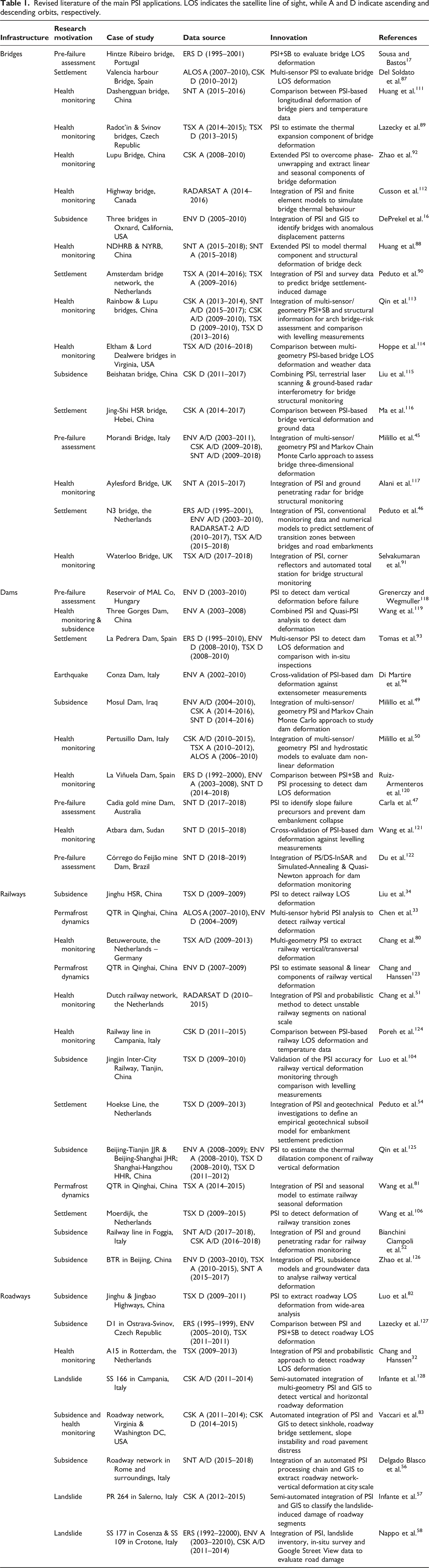
Over the last 20 years, MT-InSAR techniques have been extensively applied to the civil engineering field. A classification of the most important PSI applications for infrastructure monitoring is given in Table 1. Four infrastructure classes have been historically identified as good targets of PSI applications, nominally bridges, dams, railways and roadways. Table 1 provides relevant references for each application, including motivation, details of the study area, the space-borne InSAR sensor utilised, the acquisition geometry (ascending or descending), the period of analysis and the innovation presented in each study.

Table 1.

Revised literature of the main PSI applications. LOS indicates the satellite line of sight, while A and D indicate ascending and descending orbits, respectively.

Infrastructure	Research motivation	Case of study	Data source	Innovation	References
Bridges	Pre-failure assessment	Hintze Ribeiro bridge, Portugal	ERS D (1995–2001)	PSI+SB to evaluate bridge LOS deformation	Sousa and Bastos¹⁷
	Settlement	Valencia harbour Bridge, Spain	ALOS A (2007–2010), CSK D (2010–2012)	Multi-sensor PSI to evaluate bridge LOS deformation	Del Soldato et al.⁸⁷
	Health monitoring	Dashengguan bridge, China	SNT A (2015–2016)	Comparison between PSI-based longitudinal deformation of bridge piers and temperature data	Huang et al.¹¹¹
	Health monitoring	Radot’in & Svinov bridges, Czech Republic	TSX A (2014–2015); TSX D (2013–2015)	PSI to estimate the thermal expansion component of bridge deformation	Lazecky et al.⁸⁹
	Health monitoring	Lupu Bridge, China	CSK A (2008–2010)	Extended PSI to overcome phase-unwrapping and extract linear and seasonal components of bridge deformation	Zhao et al.⁹²
	Health monitoring	Highway bridge, Canada	RADARSAT A (2014–2016)	Integration of PSI and finite element models to simulate bridge thermal behaviour	Cusson et al.¹¹²
	Subsidence	Three bridges in Oxnard, California, USA	ENV D (2005–2010)	Integration of PSI and GIS to identify bridges with anomalous displacement patterns	DePrekel et al.¹⁶
	Health monitoring	NDHRB & NYRB, China	SNT A (2015–2018); SNT A (2015–2018)	Extended PSI to model thermal component and structural deformation of bridge deck	Huang et al.⁸⁸
	Settlement	Amsterdam bridge network, the Netherlands	TSX A (2014–2016); TSX A (2009–2016)	Integration of PSI and survey data to predict bridge settlement-induced damage	Peduto et al.⁹⁰
	Health monitoring	Rainbow & Lupu bridges, China	CSK A (2013–2014), SNT A/D (2015–2017); CSK A/D (2009–2010), TSX D (2009–2010), TSX D (2013–2016)	Integration of multi-sensor/geometry PSI+SB and structural information for arch bridge-risk assessment and comparison with levelling measurements	Qin et al.¹¹³
	Health monitoring	Eltham & Lord Dealwere bridges in Virginia, USA	TSX A/D (2016–2018)	Comparison between multi-geometry PSI-based bridge LOS deformation and weather data	Hoppe et al.¹¹⁴
	Subsidence	Beishatan bridge, China	CSK D (2011–2017)	Combining PSI, terrestrial laser scanning & ground-based radar interferometry for bridge structural monitoring	Liu et al.¹¹⁵
	Settlement	Jing-Shi HSR bridge, Hebei, China	CSK A (2014–2017)	Comparison between PSI-based bridge vertical deformation and ground data	Ma et al.¹¹⁶
	Pre-failure assessment	Morandi Bridge, Italy	ENV A/D (2003–2011), CSK A/D (2009–2018), SNT A/D (2009–2018)	Integration of multi-sensor/geometry PSI and Markov Chain Monte Carlo approach to assess bridge three-dimensional deformation	Milillo et al.⁴⁵
	Health monitoring	Aylesford Bridge, UK	SNT A (2015–2017)	Integration of PSI and ground penetrating radar for bridge structural monitoring	Alani et al.¹¹⁷
	Settlement	N3 bridge, the Netherlands	ERS A/D (1995–2001), ENV A/D (2003–2010), RADARSAT-2 A/D (2010–2017), TSX A/D (2015–2018)	Integration of PSI, conventional monitoring data and numerical models to predict settlement of transition zones between bridges and road embarkments	Peduto et al.⁴⁶
	Health monitoring	Waterloo Bridge, UK	TSX A/D (2017–2018)	Integration of PSI, corner reflectors and automated total station for bridge structural monitoring	Selvakumaran et al.⁹¹
Dams	Pre-failure assessment	Reservoir of MAL Co, Hungary	ENV D (2003–2010)	PSI to detect dam vertical deformation before failure	Grenerczy and Wegmuller¹¹⁸
	Health monitoring & subsidence	Three Gorges Dam, China	ENV A (2003–2008)	Combined PSI and Quasi-PSI analysis to detect dam deformation	Wang et al.¹¹⁹
	Settlement	La Pedrera Dam, Spain	ERS D (1995–2010), ENV D (2008–2010), TSX D (2008–2010)	Multi-sensor PSI to detect dam LOS deformation and comparison with in-situ inspections	Tomas et al.⁹³
	Earthquake	Conza Dam, Italy	ENV A (2002–2010)	Cross-validation of PSI-based dam deformation against extensometer measurements	Di Martire et al.⁹⁴
	Subsidence	Mosul Dam, Iraq	ENV A/D (2004–2010), CSK A (2014–2016), SNT D (2014–2016)	Integration of multi-sensor/geometry PSI and Markov Chain Monte Carlo approach to study dam deformation	Milillo et al.⁴⁹
	Health monitoring	Pertusillo Dam, Italy	CSK A/D (2010–2015), TSX A (2010–2012), ALOS A (2006–2010)	Integration of multi-sensor/geometry PSI and hydrostatic models to evaluate dam non-linear deformation	Milillo et al.⁵⁰
	Health monitoring	La Viñuela Dam, Spain	ERS D (1992–2000), ENV A (2003–2008), SNT D (2014–2018)	Comparison between PSI+SB and PSI processing to detect dam LOS deformation	Ruiz-Armenteros et al.¹²⁰
	Pre-failure assessment	Cadia gold mine Dam, Australia	SNT D (2017–2018)	PSI to identify slope failure precursors and prevent dam embankment collapse	Carla et al.⁴⁷
	Health monitoring	Atbara dam, Sudan	SNT D (2015–2018)	Cross-validation of PSI-based dam deformation against levelling measurements	Wang et al.¹²¹
	Pre-failure assessment	Córrego do Feijão mine Dam, Brazil	SNT D (2018–2019)	Integration of PS/DS-InSAR and Simulated-Annealing & Quasi-Newton approach for dam deformation monitoring	Du et al.¹²²
Railways	Subsidence	Jinghu HSR, China	TSX D (2009–2009)	PSI to detect railway LOS deformation	Liu et al.³⁴
	Permafrost dynamics	QTR in Qinghai, China	ALOS A (2007–2010), ENV D (2004–2009)	Multi-sensor hybrid PSI analysis to detect railway vertical deformation	Chen et al.³³
	Health monitoring	Betuweroute, the Netherlands – Germany	TSX A/D (2009–2013)	Multi-geometry PSI to extract railway vertical/transversal deformation	Chang et al.⁸⁰
	Permafrost dynamics	QTR in Qinghai, China	ENV D (2007–2009)	PSI to estimate seasonal & linear components of railway vertical deformation	Chang and Hanssen¹²³
	Health monitoring	Dutch railway network, the Netherlands	RADARSAT D (2010–2015)	Integration of PSI and probabilistic method to detect unstable railway segments on national scale	Chang et al.⁵¹
	Health monitoring	Railway line in Campania, Italy	CSK D (2011–2015)	Comparison between PSI-based railway LOS deformation and temperature data	Poreh et al.¹²⁴
	Subsidence	Jingjin Inter-City Railway, Tianjin, China	TSX D (2009–2010)	Validation of the PSI accuracy for railway vertical deformation monitoring through comparison with levelling measurements	Luo et al.¹⁰⁴
	Settlement	Hoekse Line, the Netherlands	TSX D (2009–2013)	Integration of PSI and geotechnical investigations to define an empirical geotechnical subsoil model for embankment settlement prediction	Peduto et al.⁵⁴
	Subsidence	Beijing-Tianjin JJR & Beijing-Shanghai JHR; Shanghai-Hangzhou HHR, China	ENV A (2008–2009); ENV A (2008–2010), TSX D (2008–2010), TSX D (2011–2012)	PSI to estimate the thermal dilatation component of railway vertical deformation	Qin et al.¹²⁵
	Permafrost dynamics	QTR in Qinghai, China	TSX A (2014–2015)	Integration of PSI and seasonal model to estimate railway seasonal deformation	Wang et al.⁸¹
	Settlement	Moerdijk, the Netherlands	TSX D (2009–2015)	PSI to detect deformation of railway transition zones	Wang et al.¹⁰⁶
	Subsidence	Railway line in Foggia, Italy	SNT A/D (2017–2018), CSK A/D (2016–2018)	Integration of PSI and ground penetrating radar for railway deformation monitoring	Bianchini Ciampoli et al.⁵²
	Subsidence	BTR in Beijing, China	ENV D (2003–2010), TSX A (2010–2015), SNT A (2015–2017)	Integration of PSI, subsidence models and groundwater data to analyse railway vertical deformation	Zhao et al.¹²⁶
Roadways	Subsidence	Jinghu & Jingbao Highways, China	TSX D (2009–2011)	PSI to extract roadway LOS deformation from wide-area analysis	Luo et al.⁸²
	Subsidence	D1 in Ostrava-Svinov, Czech Republic	ERS (1995–1999), ENV (2005–2010), TSX (2011–2011)	Comparison between PSI and PSI+SB to detect roadway LOS deformation	Lazecky et al.¹²⁷
	Health monitoring	A15 in Rotterdam, the Netherlands	TSX (2009–2013)	Integration of PSI and probabilistic approach to detect roadway LOS deformation	Chang and Hanssen³²
	Landslide	SS 166 in Campania, Italy	CSK A/D (2011–2014)	Semi-automated integration of multi-geometry PSI and GIS to detect vertical and horizontal roadway deformation	Infante et al.¹²⁸
	Subsidence and health monitoring	Roadway network, Virginia & Washington DC, USA	CSK A (2011–2014); CSK D (2014–2015)	Automated integration of PSI and GIS to detect sinkhole, roadway bridge settlement, slope instability and road pavement distress	Vaccari et al.⁸³
	Subsidence	Roadway network in Rome and surroundings, Italy	SNT A/D (2015–2018)	Integration of an automated PSI processing chain and GIS to extract roadway network-vertical deformation at city scale	Delgado Blasco et al.⁵⁶
	Landslide	PR 264 in Salerno, Italy	CSK A (2012–2015)	Semi-automated integration of PSI and GIS to classify the landslide-induced damage of roadway segments	Infante et al.⁵⁷
	Landslide	SS 177 in Cosenza & SS 109 in Crotone, Italy	ERS (1992–22000), ENV A (2003–22010), CSK A/D (2011–2014)	Integration of PSI, landslide inventory, in-situ survey and Google Street View data to evaluate road damage	Nappo et al.⁵⁸

The application of MT-InSAR techniques to real case studies and the cross-validation of PS-based results against in-situ measurements have demonstrated the reliability of this approach for health monitoring of different types of assets. Surface deformations can be effectively extracted for individual objects, such as buildings,^{30,31,37–40,78,79} or linear infrastructure, such as railways,^32,33,80,81 roadways,^{56,57,82–84} levees^85,86 and coastal structures.⁵⁵ Previous studies have shown the feasibility of these techniques for monitoring the settlement of bridge piers⁸⁷ and the structural deformations of bridges.^{16,45,88–92} Other studies have utilised MT-InSAR to investigate the response of dams to subsidence^48,49,93 and earthquakes,⁹⁴ or to detect the non-linear component of asset motion.^50,88

The majority of MT-InSAR validation activities have compared deformation velocities and displacement time-series with estimations based on traditional sources, such as levelling^95,96 or GPS measurements.^97–100 Accurate geolocalisation of radar targets¹⁰¹ and PS height estimate¹⁰² were demonstrated. In more recent work,^{33,34,38,103–106} InSAR-derived results from different type of structures have been compared with measurements gathered by in-situ instruments and visual inspections, revealing good agreement between the data and enabling the integration of MT-InSAR measurements with damage assessment procedures.^{38,39,107–110}

However, while these studies demonstrate the potential of MT-InSAR for infrastructure monitoring, handling the large amount of PS data for civil engineering applications is still a challenge. A significant part of the post-processing phase usually takes place using GIS, with the aim of merging the PS data and geospatial databases related to the structures within the monitored area. This allows the identification of the scatterers associated with the buildings and/or infrastructure that we want to monitor and in most of the cases it is performed manually. An automated integration of MT-InSAR data and the GIS environment will allow the capabilities of the InSAR tool to be fully exploited in order to identify anomalous moving areas^61,62 and provide early warnings,⁶⁴ with the potential to prevent future catastrophic failures on a large scale. The main novelty of this research is that the proposed methodology enables the use of InSAR deformation measurements to assess relative movements between different parts of the same infrastructure, and identify the parts of the structure that exhibit local rates and local deformation time-series dissimilar from the global structural behaviour. The proposed methodology is not limited to deformations caused by a specific source of movement.

Methodology

The proposed methodology is based on the combined use of MT-InSAR and GIS to automatically detect potential vulnerabilities along large transport networks. MT-InSAR data and a geo-spatial dataset of linear infrastructure were automatically integrated in a multistep algorithm. A velocity and displacement analysis was then performed on the given network and the results were used to produce an automatically generated report. The workflow requires two spatial datasets as an input:

• a road database in GIS file format, containing the vector data of the road centrelines;

• PS datasets, obtained after the processing of a series of InSAR images over the monitored area.

The following operations were implemented on the input datasets through an automated process:

1. Roadway identification in the GIS catalogue;

2. Preliminary integration of the two datasets by assigning the PS points to the corresponding roads;

3. Division of the roadway network into rectangular regions of equal areas;

4. Computation of PS density, average cumulative displacements and local deformation velocities for each rectangular region;

5. Generation of a report containing density, displacement and velocity maps, with specific focus on PSs showing an anomalous behaviour, that is, outliers.

The aim of the process is to (a) evaluate the spatial coverage of the InSAR-derived monitoring points, that is, PSs, on the extracted subset of roads and (b) identify critical regions and anomalous points along the network. In the rest of the paper, an anomalous PS will be referred to as an outlier, that is, a data point on a graph or in a set of results that has a significantly larger or smaller value than the next nearest data points. Figure 1 gives an overview of the analysis steps.

Figure 1.

The multistep method.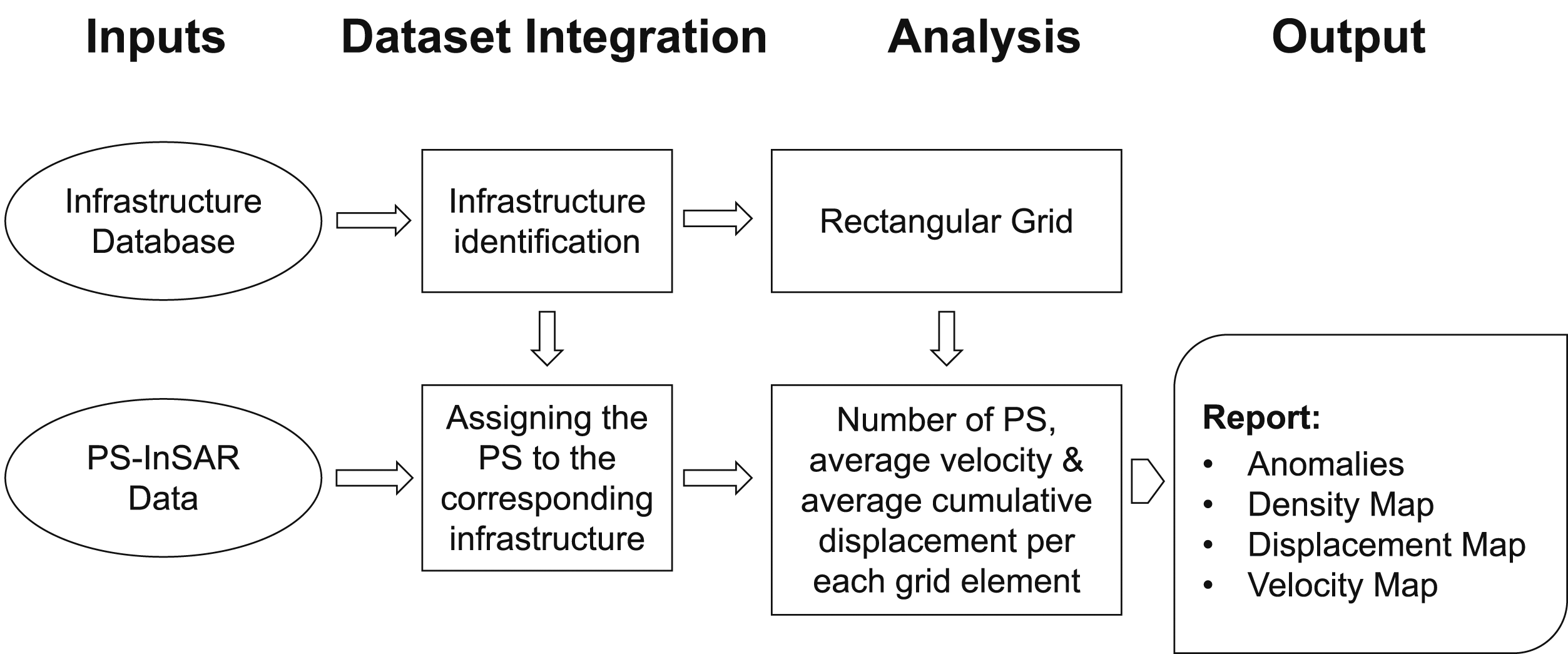

The input dataset

The algorithm shown in Figure 1 was tested on two different case studies: the Los Angeles roadway network which is subject to significant geological instabilities, and the Italian roadway system which spans a territory with a varied topography, considerable seismic and subsidence risk, and landslides of different types.

The road data used for the Los Angeles metropolitan area (Figure 2(a)) were provided by the Countywide Address Management System for Los Angeles County.¹²⁹ The Italian road data were requested to the National Geoportal of the Italian Ministry of Environment.¹³⁰ Both datasets contain the coordinates of every road, geometric measurements (such as the road length), the road name, the road type and other details. If a local database with details of the transport network in a specific area is not available, the open source OpenStreetMap (OSM) database¹³¹ could be used as an alternative.

Figure 2.

The input datasets used in the algorithm: (a) highways and freeways in Los Angeles; (b) cumulative displacement map for Los Angeles county, obtained by processing 84 ascending Sentinel images between 2016 and 2019. In (b), each PS is identified by a dot whose colour represents its cumulative displacement measured along the satellite LOS.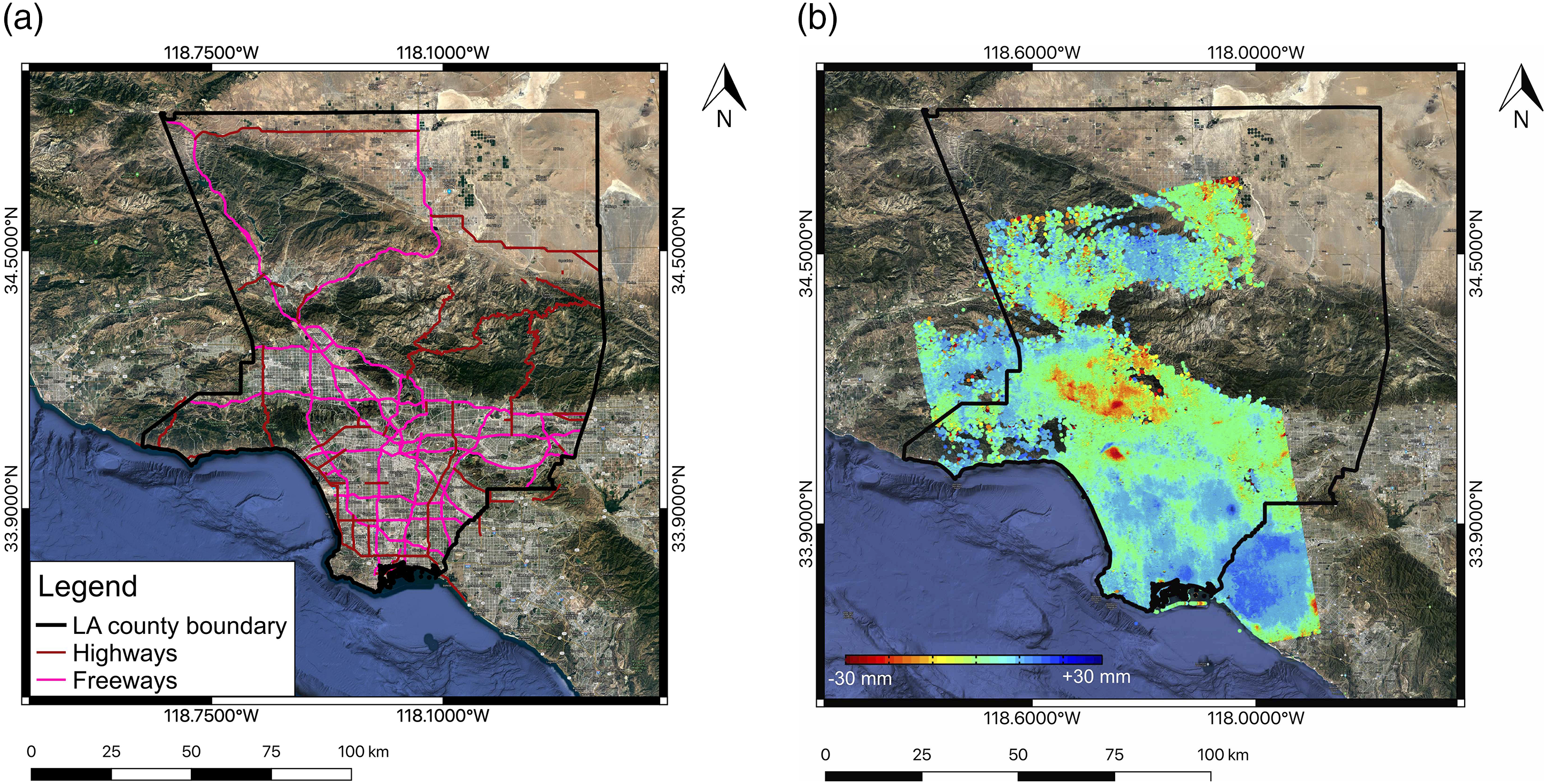

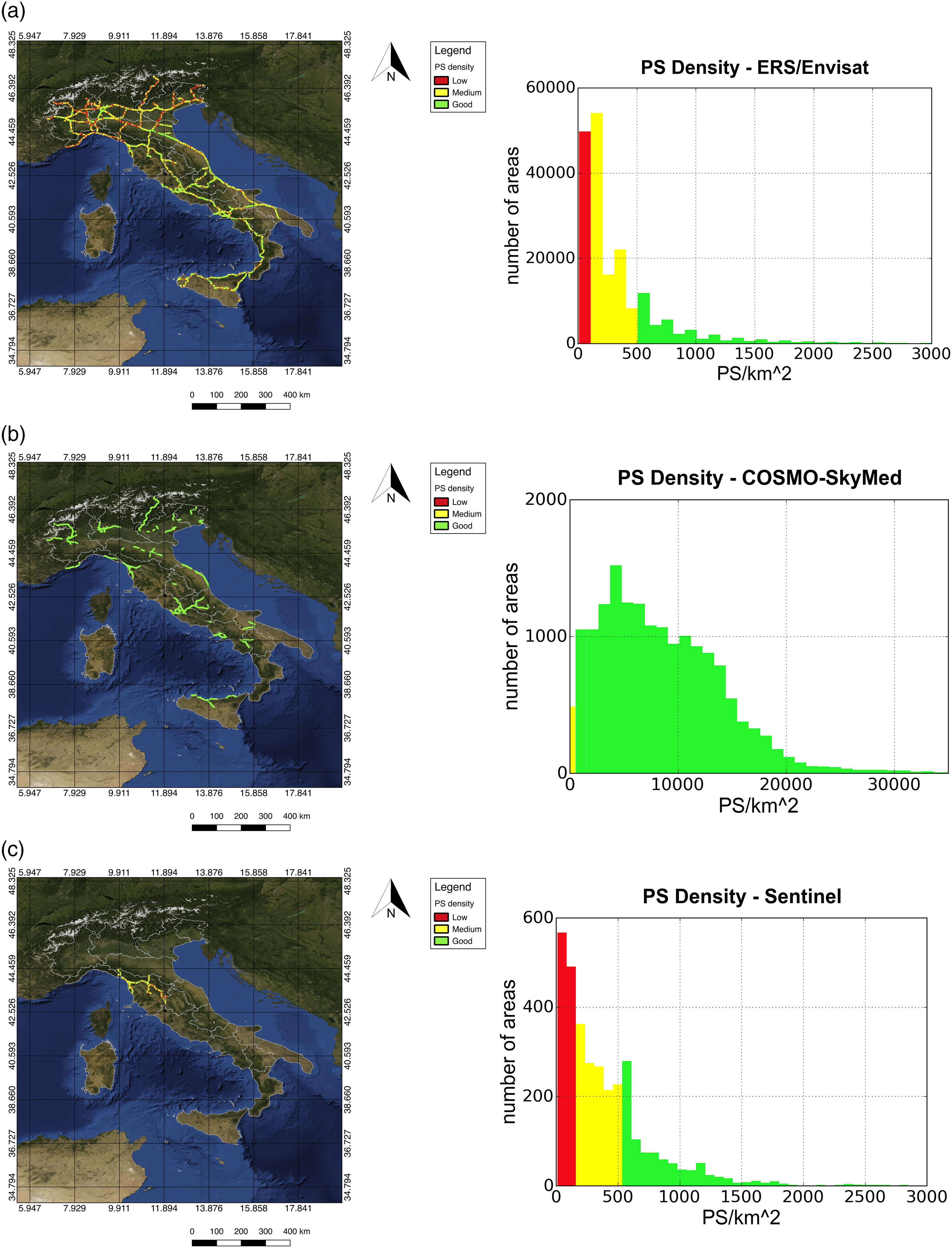
The MT-InSAR data shown in Figure 2(b) describes the cumulative displacements and the spatial location of PSs in Los Angeles County. For the Los Angeles case study, the dataset was obtained by processing 84 ascending Sentinel InSAR images from 2016 to 2019, using the SARPROZ software package.¹³² For the Italian case study, two open access PS databases were used. The first database¹³³ consists of 589 ERS/Envisat PS-datasets and 120 COSMO-SkyMed PS-datasets from both ascending and descending acquisition geometries. Such database contains surface deformation displacements over the whole Italian territory, obtained by processing the whole archive of ERS/Envisat images between 1992 and 2010 over Italy, and COSMO-SkyMed images from 2008 to 2014 for selected areas distributed over the Italian country. The second database⁶⁴ consists of seven Sentinel PS-datasets from both ascending and descending acquisition geometries, and contains surface deformations between 2014 and 2020 over the Tuscany region, in central Italy. The database published by Costantini et al.¹³³ was processed through the traditional PSI, while the datasets published by Raspini et al.⁶⁴ were processed by using the SqueeSAR technique.¹³⁴

The workflow

The first step of the algorithm was to automatically extract the roadways of the same type, that is, highways and freeways for the Los Angeles dataset and motorways for the Italian case study, from the entire road network dataset (Figures 3(a) and (b)). In order to merge the GIS and MT-InSAR datasets and identify only the PSs associated with road infrastructure, a buffer was defined around each roadway centreline (Figure 3(c)). Specifically, a 30-m-wide buffer was applied either side of the Los Angeles highways and freeways, and a 20-m-wide buffer was defined either side of the Italian motorways. The choice of a 30-m-wide buffer reflects the dimensions of the Los Angeles highways and freeways, which are characterised by a 3.7 m lane width, as defined by the U.S. Interstate Highway System, and an average number of 6 lanes per driving direction. The Italian motorway system is characterised by a number of 3 or 4 lanes per driving direction and a minimum lane width of 3.25 m, motivating the choice of a 20-m-wide buffer. If a different type of roadway is analysed, the algorithm is flexible to the use of a different buffer width. A GIS layer with roadway buffers was the first output of the analysis.

Figure 3.

Pre-processing steps: (a) the entire road network; (b) selection of a specific category of roads; (c) buffer along the road centreline.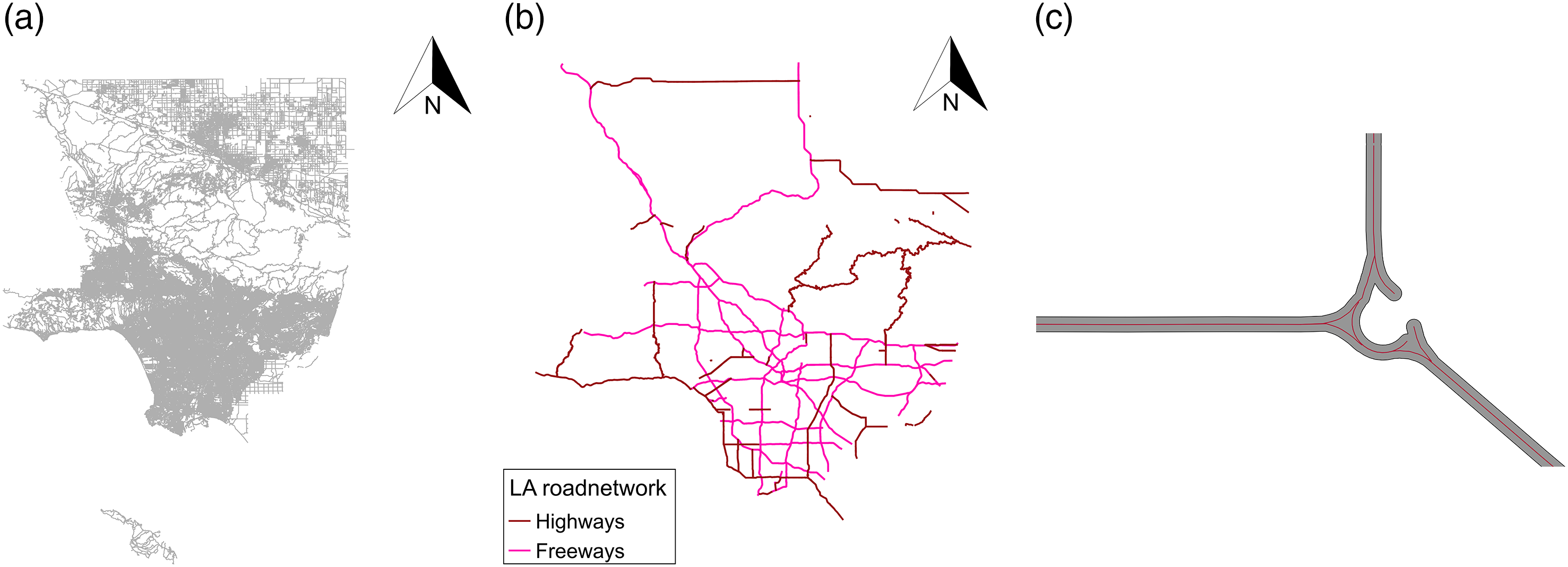

In the second step, the roadway buffer layer was used as a clipping mask and the PSs within this buffer were extracted. The displacement time-series of each PS was used to calculate deformation velocities along the satellite line of sight (LOS) for all the PSs within the buffer. Due to the differential nature of the MT-InSAR measurements, such deformation velocities are relative to a Ground Control Point (GCP) that was chosen during the MT-InSAR time-series processing. In the Los Angeles dataset, the GCP was located in a stable area of Downtown Los Angeles as in Lanari et al.¹³⁵ The Italian datasets were calibrated with GPS measurements, and more details can be found in Costantini et al.¹³³ and Raspini et al.⁶⁴ The output of this step was the PS cropped layer shown in Figure 4. Deformation velocities were stored in the attribute table of this layer. The geographical coordinates of the PS cropped layer extent were used to identify only the roadways contained in the area for which the PS data is available.

Figure 4.

Permanent Scatterers (PSs) cropped on the Los Angeles highway and freeway network. The map shows the cumulative displacements on the infrastructure, measured along the satellite LOS between 2016 and 2019. Each PS is identified by a dot whose colour represents its LOS cumulative displacement. Negative values correspond to PSs moving away from the satellite, while positive values refer to displacements toward the satellite.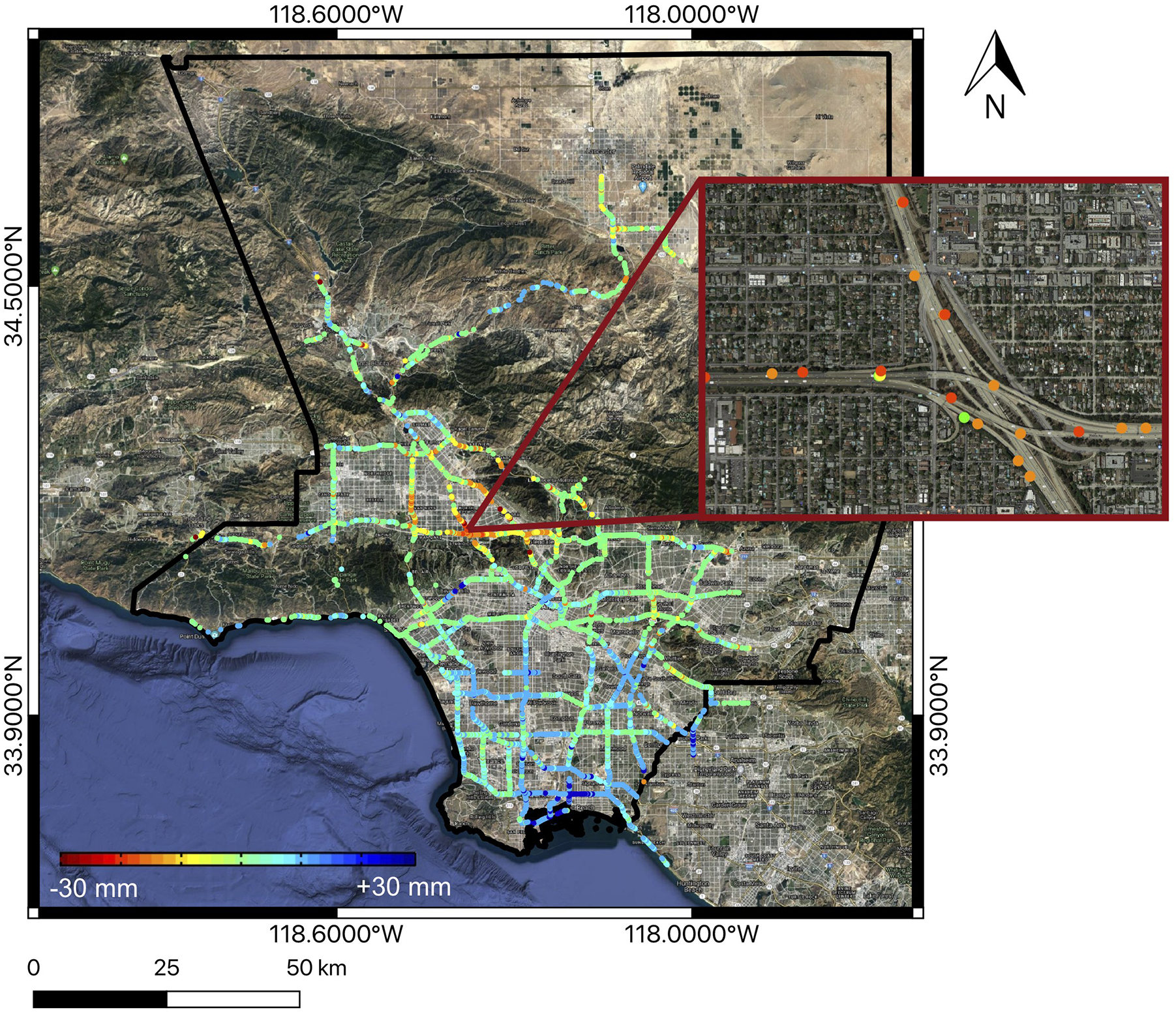

In the third step, a rectangular grid was created along the linear infrastructure to quantify the density of monitoring points (PSs) and identify critical locations. Specifically, each road centreline was split into equal segments of 500-m-length. This value was selected for practical reasons. Due to the diverse ground resolution of different SAR sensors,⁶³ an analysis based on a rectangle with a shorter side would lose statistical significance. Conversely, a rectangle with a longer side cannot accurately follow the shape of the roadway. Then, rectangles of equal area, as wide as the buffer previously applied, were built around each segment. It is noted that the width of the rectangle can be modified according to the type of roadway under analysis. The rectangles were rotated such that they are aligned to their respective road segment, allowing the grid to adapt its shape to the corresponding infrastructure. The rectangular grid is shown in Figure 5.

Figure 5.

Example of rectangular grid along linear infrastructure.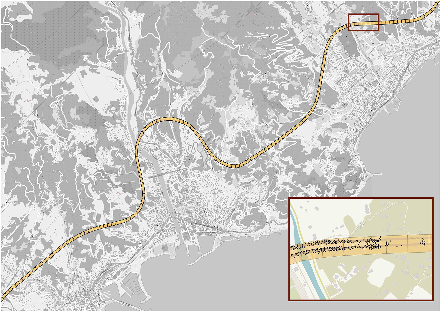

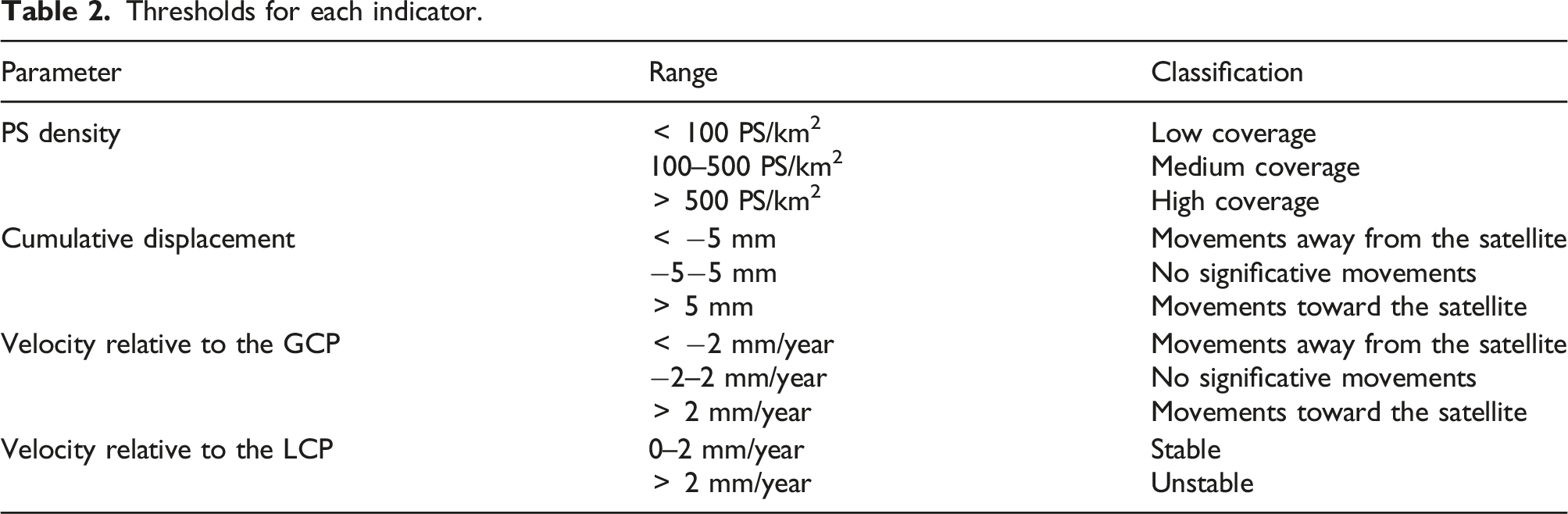
In the fourth step, outputs from the previous phase, that is, the PS cropped layer and the rectangular grid, were used to identify the PSs contained in each rectangle. This information was used to calculate the PS density (number of PS per km²), the average deformation velocity, the average cumulative displacement and the average value of the displacement time-series for each rectangle. Average cumulative displacements and average deformation velocities were firstly calculated with respect to the GCP. To reduce uncompensated noise due to a distant GCP and remove possible seasonal effects and local instabilities, a Local Control Point (LCP) was identified for each rectangle. Since deformation velocities were already calculated during step 2, the LCP was selected as the slowest moving point along the satellite line of sight in each rectangle. Deformation time-series and absolute values of velocities relative to this point were calculated for all other PSs within the rectangle. Finally, an average velocity relative to the LCP was assigned to each rectangle. The outputs from this step were a GIS layer containing the rectangular grid and a GIS layer containing the LCPs. All the information concerning density, average deformation velocities and average cumulative displacements with respect to the GCP, average velocities relative to the LCPs and displacement time-series were stored in an attribute table of the generated GIS layers and used in the final step to generate corresponding maps and histograms. For each rectangle, a clustering approach was used to detect potential outliers, that is, PSs with a relative deformation rate higher than a given threshold and a relative deformation time-series dissimilar from the global structural behaviour. Specifically, to identify the outliers three criteria were implemented:

1. for each rectangle, a PS was classified as an outlier if the absolute value of its relative velocity |v| with respect to the LCP is higher than 5 mm/year. Specifically, three ranges were defined: 5–7 mm/year, 7–9 mm/year and $>$ 9 mm/year. The selected thresholds are in line with previous studies⁶⁴;

2. the Average Local Displacement (ALD), that is, the mean value of the displacement time-series, was calculated for each rectangle as the mean of the displacement time-series of all the PSs within the rectangle. Outliers were identified as those exceeding the standard deviation of the ALD in the last 2 years of the InSAR dataset’s time frame;

3. the Median Local Displacement (MLD), that is, the median value of the displacement time-series, was calculated as the median of the displacement time-series of all the PSs within the rectangle. Outliers were identified as those exceeding the standard deviation of the MLD in the last 2 years of the InSAR dataset’s time frame.

It should be noted that the presence of outliers is not a straightforward indicator of a severe structural condition, but only highlights an unusual behaviour that needs to be investigated. All the outliers and related information were saved in different GIS layers.

In the fifth and final step of the algorithm, the analysis performed in the previous step was summarised in maps and histograms showing the density distribution, deformation velocities and cumulative displacements over the monitored area. Thresholds were defined for each parameter to identify the ranges of values shown in Table 2. Specifically, to evaluate the density of PSs among different parts of the network, three ranges of density based on the number of PS per km² were defined. A low coverage refers to a density lower than 100 PS/km², medium coverage corresponds to a density range between 100 PS/km² and 500 PS/km² and good coverage refers to a PS density higher than 500 PS/km². These ranges were based on the dimension of the rectangular grid built along the roadway infrastructure, and are in line with observations presented in previous studies.^37,56,62,82 Cumulative displacements between −5 mm and 5 mm and deformation rates between −2 mm/year and 2 mm/year, both relative to the GCP, indicate no significative movements along the satellite line of sight. Positive and negative values indicate movements toward and away from the satellite, respectively. For relative velocities with respect to the LCPs, values larger than 2 mm/year are assumed to indicate an unstable condition. The displacement and velocity thresholds adopted in this study are in line with classification values already presented in literature.^{63,64,136,137} On the basis of these ranges, a different colour was assigned to each rectangle defined during step 3, and used to render density, displacements and velocity maps. Maps showing the outlier distribution were also generated.

Table 2.

Thresholds for each indicator.

Parameter	Range	Classification
PS density	$<$ 100 PS/km²	Low coverage
	100–500 PS/km²	Medium coverage
	$>$ 500 PS/km²	High coverage
Cumulative displacement	$<$ −5 mm	Movements away from the satellite
	−5−5 mm	No significative movements
	$>$ 5 mm	Movements toward the satellite
Velocity relative to the GCP	$<$ −2 mm/year	Movements away from the satellite
	−2–2 mm/year	No significative movements
	$>$ 2 mm/year	Movements toward the satellite
Velocity relative to the LCP	0–2 mm/year	Stable
Velocity relative to the LCP	$>$ 2 mm/year	Unstable

The MT-InSAR processing chain: improvements adopted in this paper

The MT-InSAR datasets used in this paper were processed following the core steps of Permanent Scatterer Interferometry (PSI).^24,25 PSI involves a series of N InSAR images and the goal are the identification of pixels showing stable scattering properties over the whole set of images, that is, PSs, and the retrieval of their time-motion.

The PSI analysis is usually performed by assuming a linear target motion, meaning that coherent scatterers characterised by a non-linear motion are not identified as PSs, or that the non-linear component of the their motion is identified as part of the atmospheric contribution.²⁴ Furthermore, Perissin and Wang¹³⁸ observed that sometimes only a limited number of targets behave coherently along the whole observation span, limiting the applicability of PSI techniques. This is particularly true outside of urbanised areas where coherent targets can be surrounded by vegetation or water basins, or when PSs are partially coherent during the observation span. This latter case is verified during the construction of new structures or the demolition of old ones, leading to a certain number of PSs appearing or vanishing.¹³⁹ Consequently, in some scenarios a limited availability of PSs per structure or a full lack of coverage for certain assets can be observed, limiting the PSI performance for structural deformation analysis on large scale.

To increase the PS density on man-made objects, the Sentinel dataset used for the analysis of Los Angeles bridges (the section ‘Bridges and Viaducts in Los Angeles’) was processed by adding a step between steps 1 and 2 (Figure 6) of the traditional PSI processing chain.²⁵ This step, indicated as 1b, exploits the spatial location of the selected pixels to increase the initial number of PS candidates, and originates from the idea presented by Van Leijen¹⁴⁰ of applying a rectangular mask to the data for initial pixel selection. The flowchart of Figure 6 provides an overview of the improved processing chain.

Figure 6.

Steps of the improved PSI processing chain.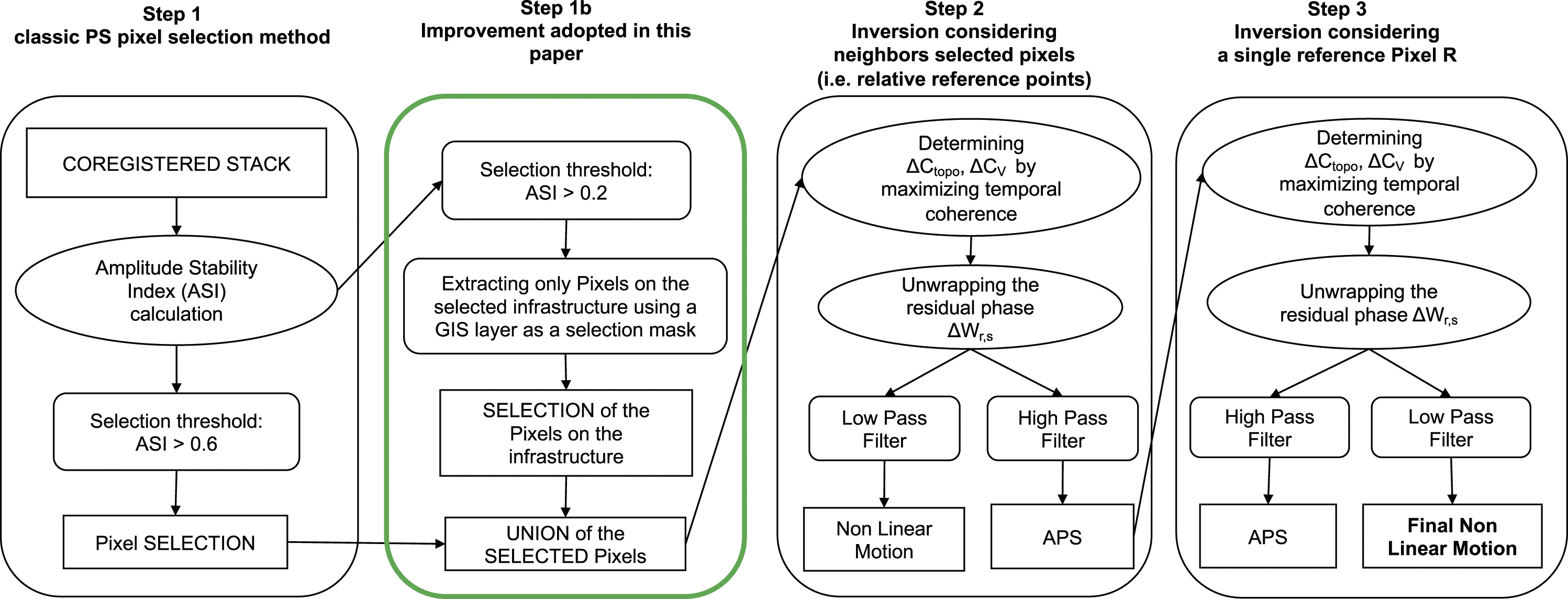

In step 1, PS candidates were identified on the basis of their amplitude stability index (ASI). For a given pixel k, the ASI quantifies the stability of the pixel amplitude values along the temporal series of InSAR images. The mean and standard deviation of the pixel amplitudes along the N InSAR images are represented by μ_k and σ_k, respectively, with the pixel ASI defined as⁷⁷

ASI = 1 - \frac{σ_{k}}{μ_{k}} .

(1)

The ASI was estimated for each pixel, and only pixels with ASI greater than a certain threshold, that is, ASI $>$ 0.6, were selected. This assumption enabled the identification of an initial number of PSs, and more PSs were selected during the rest of the processing. An initial set of selected pixels was the output of this step.

In step 1b, the ASI threshold was reduced to 0.2. Then, a GIS buffer layer containing the buffer of the infrastructure network, as defined in the section ‘The workflow’, was overlapped to the pixels with reduced ASI, and only the pixels within the buffer were selected. This operation is based on the observation that even pixels with a low ASI can be characterised by high temporal coherence. In addition, the exploitation of the GIS buffer layer gives confidence that the pixels with lower ASI belong to the infrastructure. This operation enabled the selection of an increased number of pixels on the infrastructure network. Then, the PS candidates from step 1 were integrated with the pixels selected in step 1b. The union of the two set of pixels is the output of this step.

Lastly, steps 2 and 3 (Figure 6) of the traditional PSI processing chain were resumed to determine the displacement-temporal series of the selected pixels.

Case studies

The Los Angeles case study

Los Angeles County is the second largest metropolitan area in the United States and the region with the densest road network in the country.¹⁴¹ Most of the existing roadway infrastructure (around the 80%) was deployed before 1960 and the 90% of current roadways were built by 1987.¹⁴² Today the growth of the urban infrastructure system is minimal. The network consists of approximately 39,000 centreline road kilometres, with local roads accounting for 76% of the total network. Handling the maintenance of a such large network is critical. Government institutions are constantly struggling to finance the maintenance of the existing road-infrastructure and the costs often exceed the city budget.¹⁴³ It is estimated that the construction of the network costed approximately $30 billion and maintenance activities have cost a $49 billion of investment since it was constructed. In particular, since 1987, the average annual maintenance cost is estimated at $1 billion and, on average, the construction and maintenance of the network has cost approximately $2 million per centreline kilometre.¹⁴⁴

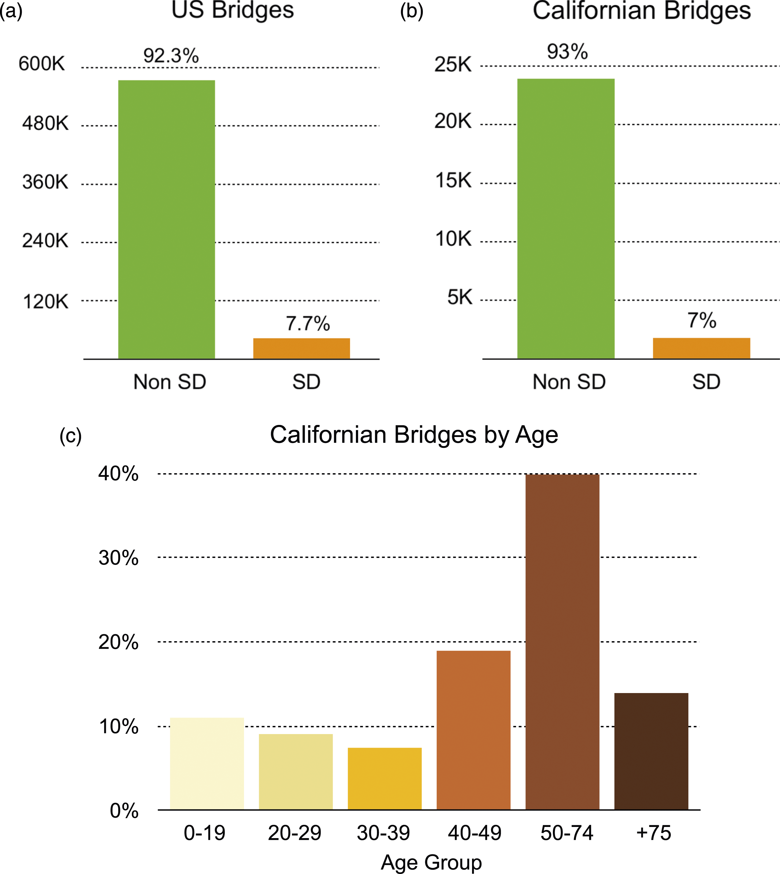
In its 2019 Bridge Report,⁶ the American Road & Transportation Builders Association rated 47 052 of America’s 616 087 bridges as ‘structurally deficient’ (Figure 7(a)). In California, 1812 bridges – about the 7% of the bridges in the State – were classified as structurally deficient (Figure 7(b)) and 5093 bridges need repairs for an estimated cost of $8.8 billion.¹⁴⁵ Los Angeles County is home to five of the California’s 10 most-travelled structurally deficient bridges – two of them are along Highway 101 and the other three are on the Interstate 405. According to the American Society of Civil Engineers,¹⁴⁶ over 50% bridges in the state exceeded their design life, making California the US state with the second largest number of outdated bridges. Many bridges currently in service were designed for a 50-year lifespan and the average age of the structurally deficient bridges is 62 years. 53% Californian bridges are over 50 years old and 13% exceed 75 years in age (Figure 7(c)).

Figure 7.

Structurally deficient (SD) bridges in (a) US and (b) California. (c) Classification of 25 701 Californian bridges by age.¹⁴⁶

The Italian case study

In Italy, the construction of the modern roadway network started in the late 19th century, but most major roads were built between 1950 and 1980.¹⁴⁷ Since the 50s, the motorway system expanded rapidly, increasing from 500 km to over 6000 km in the 80s and becoming the second largest motorway network in Europe. Between 1950 and 1980, national and secondary roads increased by 72%.¹⁴⁸ Nowadays, the overall network consists of about 7000 km of motorway (fourth in Europe after Spain, Germany and France), 20,000 km of national roads and over 155,000 km of secondary and regional roads, accounting for 85% of the all roads in the country. The maintenance of the overall Italian network is estimated to cost about €24.4 billion per year, corresponding to €30,000 per km of road. The motorway infrastructure expenditure is about €5.4 billion per year.¹⁴⁹

The Italian transport infrastructure includes about 43,000 road bridges and more than 1034 km of motorway bridges and viaducts.¹⁵⁰ According to Occhiuzzi,¹⁵¹ tens of thousands of bridges and viaducts were built in the 1950s and 60s, and are currently beyond their expected lifespan. In addition, approximately 70% of Italy’s 15,000 motorway bridges and tunnels are today more than 40 years old. The cost of a single bridge is typically €2000 per m² and it is estimated that tens of billions of euros are required to upgrade Italy’s aged infrastructure.

Results

Los Angeles and Italian roadway networks

The algorithm described in the section ‘The workflow’ was applied to two road networks using different InSAR sensors. A single Sentinel dataset from 2016 to 2019 was used to monitor the Los Angeles highway and freeway network. Seven Sentinel PS-datasets between 2014 and 2020 were used to analyse the Italian motorway in the Tuscany region, Italy, and 589 ERS/Envisat PS-datasets between 1992 and 2010 and 120 COSMO-SkyMed PS-datasets between 2008 and 2014 were used for the entire Italian motorway system. The application of the algorithm to these two case studies resulted in the automated creation of a report (step 5) which contains maps and histograms showing the distribution of PS densities, average cumulative displacements relative to the GCP, average velocities relative to the GCP and LCPs, and outliers. Depending on the number of outliers, additional details on the anomalous points are provided. Specifically, for each road segment containing at least one outlier, a close-up map of the critical road-segment and three plots showing the displacement time-series of the LCP, the displacement time-series of the fastest anomalous point, and the relative displacement time-series of the fastest anomalous point with respect to the LCP are displayed.

For Los Angeles, the analysis was performed on 4978 centreline kilometre of highway and freeway, and 10 117 Sentinel PSs and about 1 million displacement measurements were identified over the road infrastructure. The Italian motorway network consists of about 14, 600 centreline kilometre. The ERS/Envisat datasets provided over 286, 000 PSs and 14 million displacement measurements over the Italian motorway network, the COSMO-SkyMed datasets enabled the identification of about 1.5 million PSs and 69 million displacement measurements on the infrastructure, and the Sentinel datasets in the Tuscany region, Italy, provided 11, 276 PSs and about 3 million displacement measurements on the network. The application of the algorithm to test areas with such different extent and characteristics demonstrates how the proposed methodology can be applied from city to national scale.

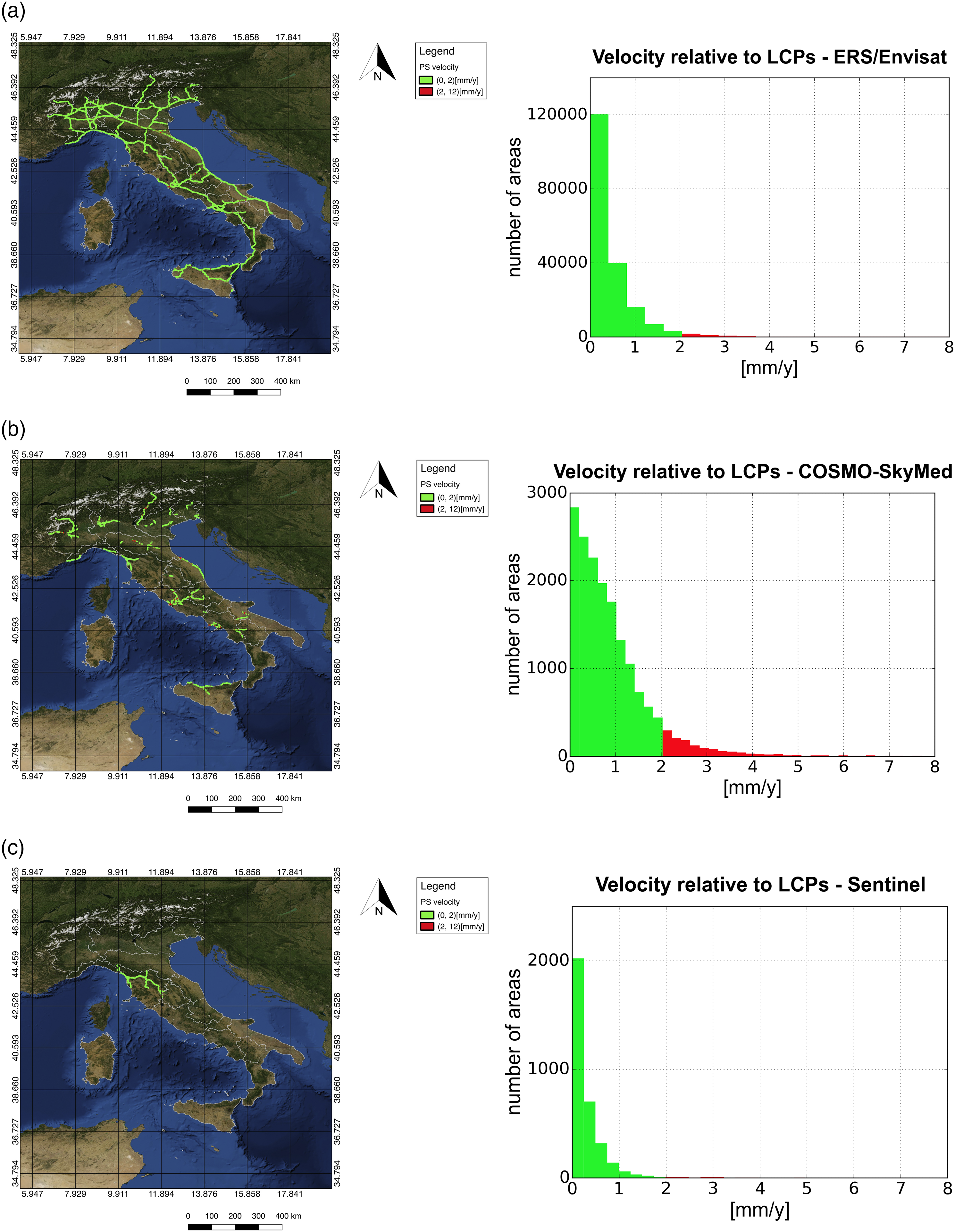
The maps and histograms in Figures 8, 9 and 12(a) show the density distribution of the PS extracted over the linear infrastructure, providing a global overview of the number of scatterers along the network and highlighting the areas with more monitoring points. It is noted that when two acquisition geometries were available, PS densities were estimated for each acquisition geometry. The PS density along different parts of the network was evaluated using the three categories of density defined in the section ‘The workflow’. The Sentinel dataset in Los Angeles provides an average number of 326 PS/km² and indicates that almost 60% road segments have medium density of PS, while 19% of road segments have a good PS density and 21% of the area has a low number of PS per km² (Figures 8 and 12(a)). As already observed in previous studies,^74,152 high-resolution satellites – that is, COSMO-SkyMed – provide a higher number of permanent scatterers. In the case of ERS/Envisat data (Figures 9(a) and 12(a)), about 79% of road segments are covered by less than 500 PS/km² with an average number of 364 PS/km², while the COSMO-SkyMed dataset (Figures 9(b) and 12(a)) provides an average number of 8400 PS/km² and 97% of road segments have a good PS-density, that is, higher than 500 PS/km². The Sentinel dataset in the Tuscany region, Italy, provides an average number of 417 PS/km²: 55% of road segments have a medium PS-density, 28% of road segments have a good PS-density and 17% of road segments are characterised by a low PS-density (Figures 9(c) and 12(a)). Due to the different spatial scale of the two networks and the exploitation of a different number of datasets, the Los Angeles and the Italian case studies cannot be directly compared, but the PS densities provided by Sentinel and ERS/Envisat is similar. It is also noted that the Sentinel dataset in Los Angeles refers to a single acquisition geometry, that is, ascending, while for the Italian case study, ERS/Envisat and Sentinel datasets from both ascending and descending orbits were used.

Figure 8.

PS density over the Los Angeles highway and freeway network using Sentinel-1 data from 2016 to 2019.

Figure 9.

PS density over the Italian motorway network using (a) ERS/Envisat data from 1992 to 2010, (b) COSMO-SkyMed data from 2008 to 2014 and (c) Sentinel-1 data from 2014 to 2020 in the Tuscany region. For visualisation purpose, a different scale interval was adopted for the x-axis.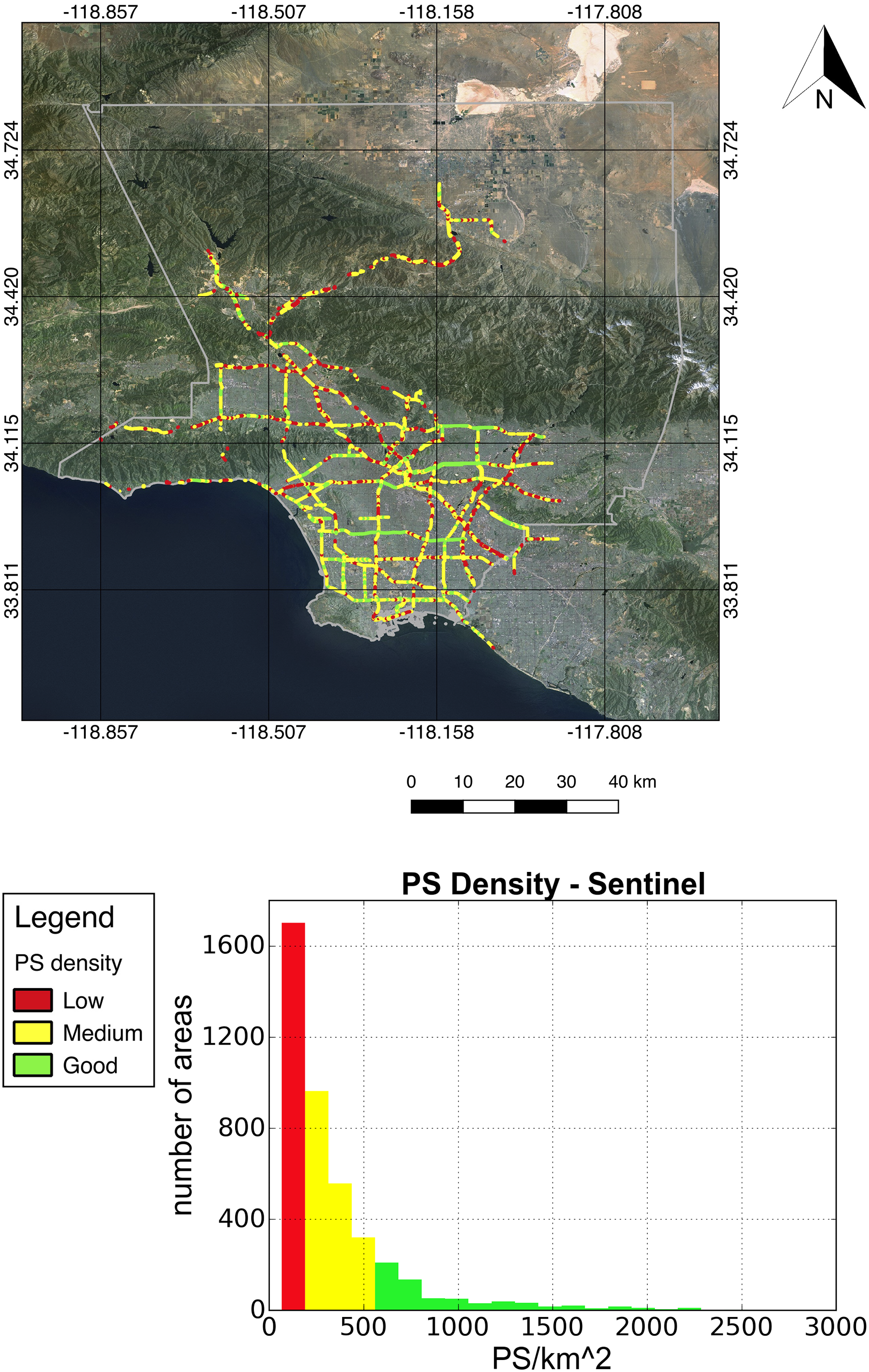

To remove seasonal effects and regional instabilities due to a distant ground reference point (GCP), velocity maps referred to LCPs (Figures 10 and 11) were generated. The maps show in red the road segments deforming at a rate higher than 2 mm/year, allowing critical locations to be identified. Figure 12(d) summarises the information displayed in Figures 10 and 11, showing instability for 3% of the Los Angeles network. For the Italian motorway, 2.2% of the network is classified as unstable when the ERS/Envisat data are used, the COSMO-SkyMed data reveal instability for 8.4% of the network, and the Sentinel data in the Tuscany region show instability for about 1% of the network. The different distribution of these indicators can be explained by the different temporal window and surface extension of ERS/Envisat, COSMO-SkyMed and Sentinel data and the higher PS density provided by the COSMO-SkyMed datasets.

Figure 10.

Distribution of relative velocities referred to Local Control Points over the Los Angeles highway and freeway network using Sentinel-1 data from 2016 to 2019. The proposed classification is based on relative velocity absolute values.

Figure 11.

Distribution of relative velocities referred to Local Control Points over the Italian motorway network using (a) ERS/Envisat data from 1992 to 2010, (b) COSMO-SkyMed data from 2008 to 2014 and (c) Sentinel-1 data from 2014 to 2020 in the Tuscany region. The proposed classification is based on relative velocity absolute values. For visualisation purpose, the same scale interval was adopted for the x-axis.

Figure 12.

Percentage distribution of (a) PS density, (b) cumulative displacements, (c) velocities related to the GCP and (d) relative velocities related to LCPs, over Los Angeles using Sentinel data from 2016 to 2019 and over Italy using Sentinel, ERS/Envisat and COSMO-SkyMed data from 2014 to 2020, from 1992 to 2010 and from 2008 to 2014, respectively.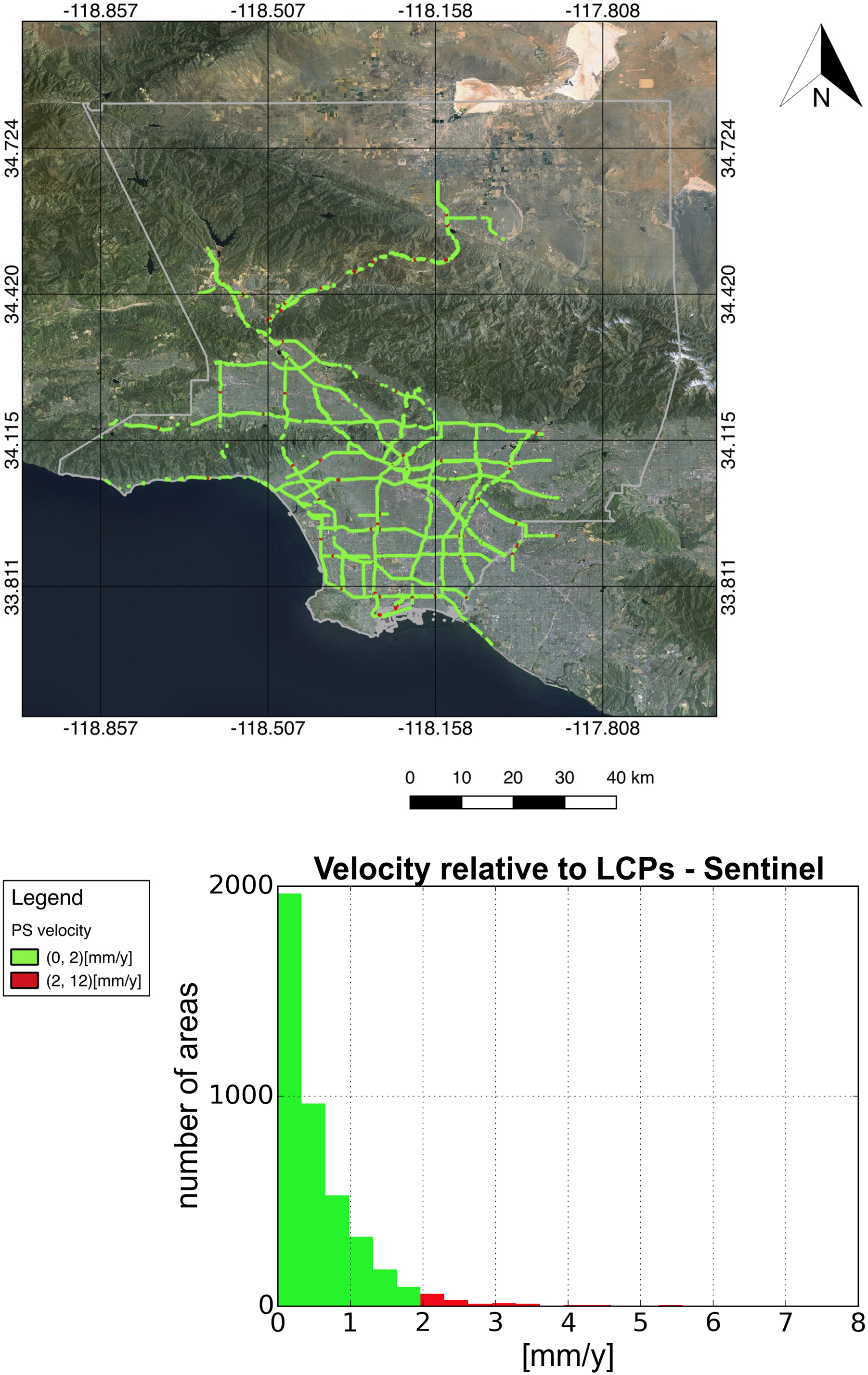

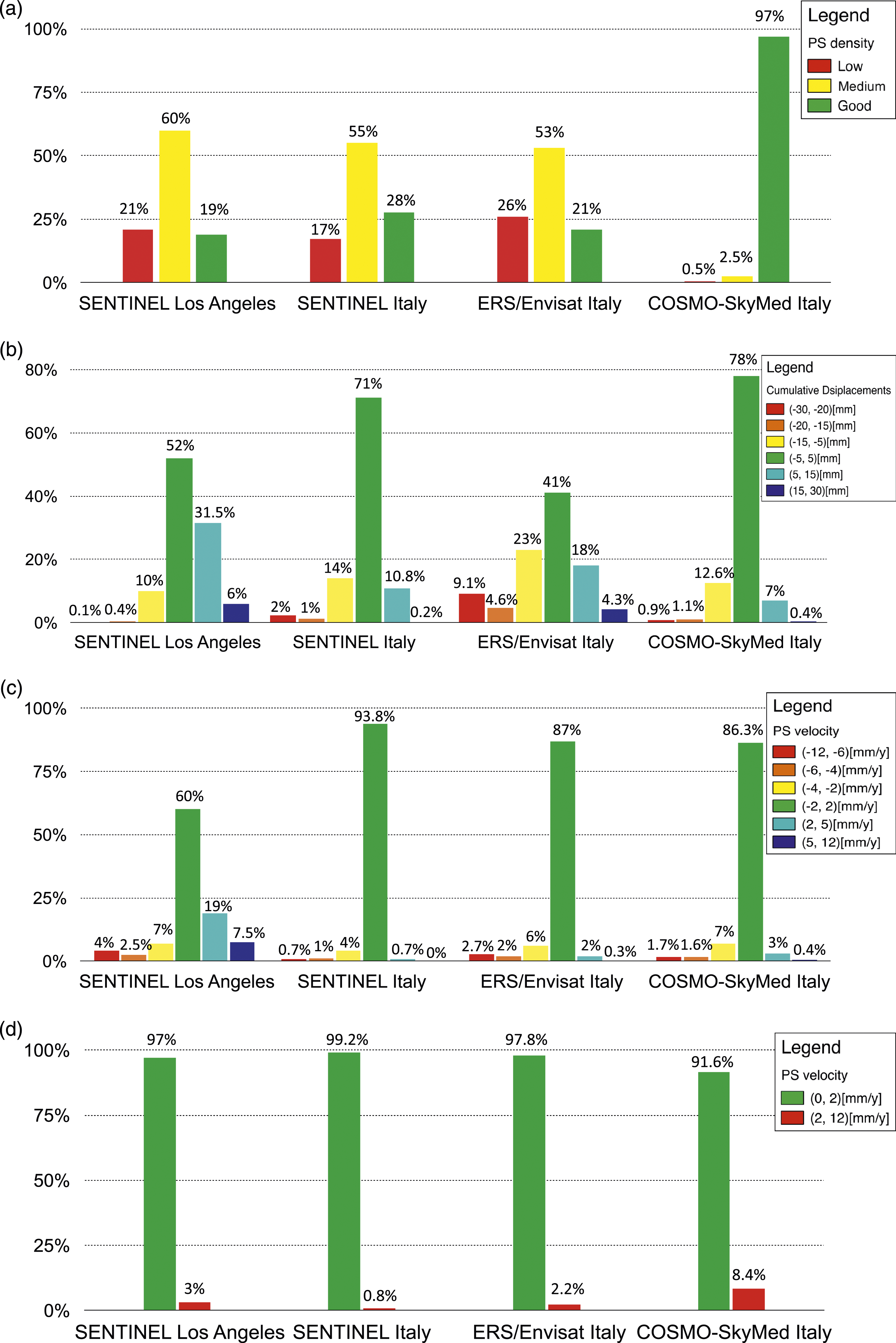
Figures 12(b) and (c) summarise the cumulative displacement and velocity distribution with respect to a GCP over the Los Angeles and Italian road networks. About 6% of the Los Angeles network exhibits movements larger than 15 mm and a velocity higher than 5 mm/year, while for about 11% of the network movements away from the satellite can be observed. The Italian network is mainly dominated by an average velocity between −2 mm/year and 2 mm/year: about 87% of road segments is in this range for both ERS/Envisat and COSMO-SkyMed datasets. The ERS/Envisat datasets reveal movements toward the satellite for about 22% of road segments and movements away from the satellite for about 37% of the network. The COSMO-SkyMed data shows high displacements away from the satellite for 15% of the network and movements toward the satellite for 7.4% of road segments. Similarly, the Sentinel datasets over the Tuscany region show that about 94% of road segments are characterised by average velocities between −2 mm/year and 2 mm/year, and reveal movements toward and away from the satellite for 11% and 17% of road segments, respectively.

The distribution of outliers over the monitored areas is shown in Figure 13. The Sentinel data in Los Angeles led to the identification of 88 outliers along the Los Angeles highways and freeways (Figure 13(a)). 14% of these points have a local velocity higher than 9 mm/year, 10% are in the range 7 mm/year to 9 mm/year, and the remaining 76% have a velocity between 5 mm/year and 7 mm/year (Figure 13(e)). For the Italian case study, the Sentinel datasets over the Tuscany region led to the identification of 25 outliers along the Italian motorway; and 84% of them is characterised by local velocity between 5 mm/year and 7 mm/year (Figure 13(b) and (e)). The use of multiple ERS and Envisat datasets revealed 2525 outliers over the Italian motorway network (Figure 13(c)). 70% of the outliers show local velocity between 5 mm/year and 7 mm/year, 16% between 7 mm/year and 9 mm/year and the last 14% exceeds 9 mm/year (Figure 13(e)). The COSMO-SkyMed dataset revealed 27 602 outliers (Figures 13(d) and (e)), corresponding to a factor of 10 more outliers than ERS/Envisat. This is explained by the higher density of PSs that is achieved with high-resolution X-band SAR satellites, that is, COSMO-SkyMed, with respect to low or medium-resolution satellites operating in the C-band, that is, ERS/Envisat.^26,74 Figure 13(e) shows that 59% of these outliers have a relative velocity between 5 mm/year and 7 mm/year, 21% are in the range 7 mm/year–9 mm/year and 20% have a relative velocity higher than 9 mm/year.

Figure 13.

Outliers (a) in Los Angeles using Sentinel data from 2016 to 2019, (b) in the Tuscany region, Italy, using Sentinel data from 2014 to 2020, (c) in Italy using ERS/Envisat data from 1992 to 2010 and (d) in Italy using COSMO-SkyMed data from 2008 to 2014. (e) Percentage distribution of the outliers over the four datasets. Depending on the absolute value of their relative velocity v related to LCPs, the outliers are indicated with yellow, orange or red dots.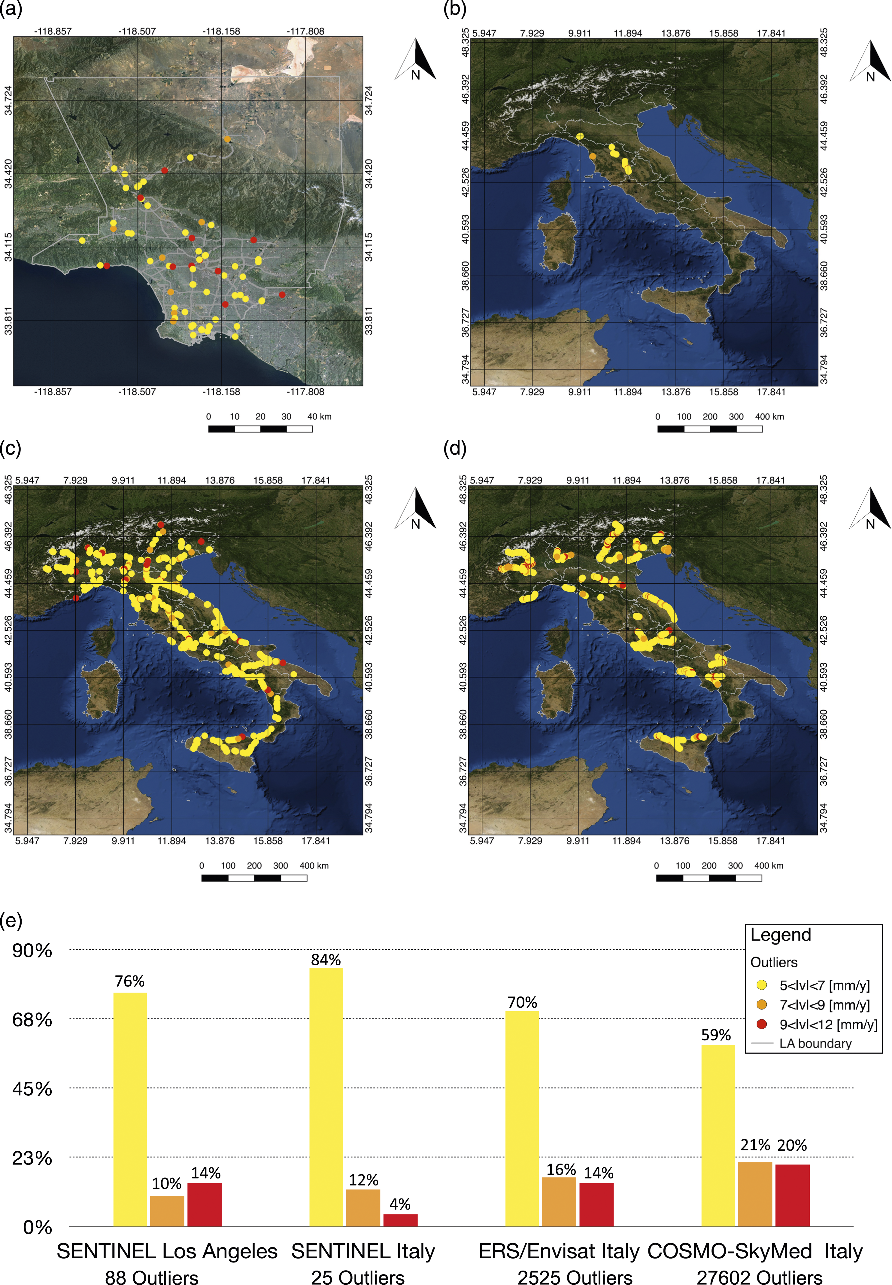

Table 3 summarises the results of the analysis showing for each SAR sensor the number of PSs, displacement measurements and outliers identified on the corresponding roadway infrastructure, and the average number of PSs per km² of infrastructure.

Table 3:

Comparison between ERS/Envisat (ERS/ENV), COSMO-SkyMed (CSK) and Sentinel (SNT) for the analysis of the Italian motorway network, and Sentinel for the analysis of the Los Angeles highway and freeway network.

InSAR sensor	Temporal window	Number of PSs on infrastructure	Number of displacement measurements	Average PSs/km² of infrastructure	Outliers
SNT (Los Angeles)	2016–2019	10,117	1 million	326	88
ERS/ENV (Italy)	1992–2010	286,000	14 million	364	2525
CSK (Italy)	2008–2014	1.5 million	69 million	8400	27,602
SNT (Tuscany, Italy)	2014–2020	11,276	3 million	417	25

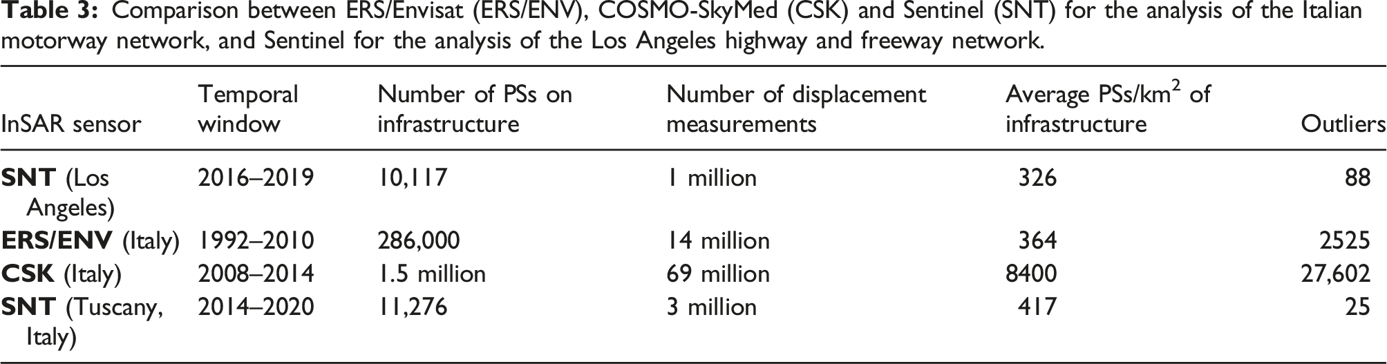
Figure 14 shows an example of a specific outlier. The map (Figure 14(a)) shows the location of the outlier, and its displacement time-series between 2016 and 2019 is shown in Figure 14(b). The deformation pattern of Figure 14(c) is obtained by subtracting the displacement time-series of the LCP (Figure 14(d)) to the displacement time-series of the outlier, and indicates that the outlier moved about 3 cm with respect to the LCP between October 2016 and February 2017. The light and dark grey bands indicate the ranges within which 68% and 95% of values lie, respectively, and show that since the early 2017 the detected outlier is more than two standard deviations (2σ) away from the mean displacement time-series.

Figure 14.

Details of a critical location: (a) map showing the area of interest, with a specific outlier in red, Local Control Point (LCP) in light blue and other PSs (Permanent Scatterers) in black; (b) displacement time-series of the point with highest relative velocity in black; (c) relative displacement time-series of the same point with respect to the LCP in black; (d) displacement time-series of the LCP in black. The red line refers to the average displacement time-series, obtained as the mean of the displacement time-series of all the PSs in the rectangle. The light and dark grey bands indicate one (σ) and two (2σ) standard deviations from the average displacement time-series, respectively.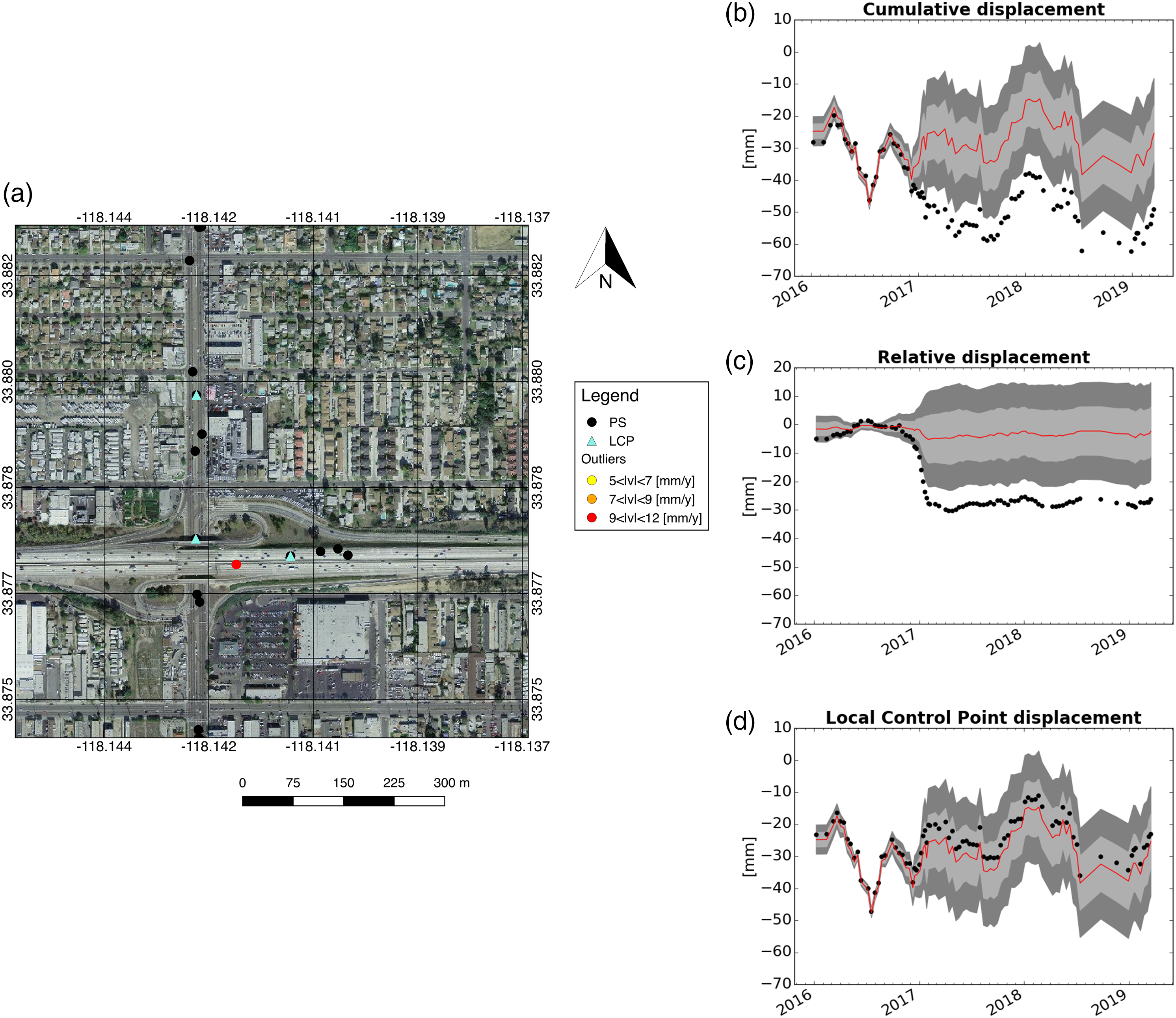

Bridges and Viaducts in Los Angeles

To demonstrate that the proposed methodology is flexible to the analysis of different infrastructure classes, the algorithm described in the section ‘The workflow’ was applied to Los Angeles roadway bridges, using the Sentinel dataset over Los Angeles County as an input (see the section ‘The input dataset’). The OpenStreetMap dataset for the Californian roadway network was used in this section to identify the footprints of roadway bridges in the California State.

To improve the spatial density of PSs, the series of Sentinel images already used for the Los Angeles freeway and motorway network was processed using the methodology described in the section ‘The MT-InSAR processing chain: improvements adopted in this paper’. The improved PSI processing chain allowed for over double the number of bridges to be monitored. Figure 15 shows the PS-density distribution over the Los Angeles bridges obtained through the implemented improvement. For the original dataset, PSs were retrieved for only 1373 bridges, while with the improved processing at least one monitoring point is available for 3110 bridges, and 60.6% of them exhibit 3 or more monitoring points.

Figure 15.

PS density over roadway bridges in Los Angeles based on Sentinel data from 2016 to 2019, using the improved PSI processing chain (the section ‘The MT-InSAR processing chain: improvements adopted in this paper’). Each asset is identified by a star symbol and a green star indicates the assets for which at least 3 PS were observed.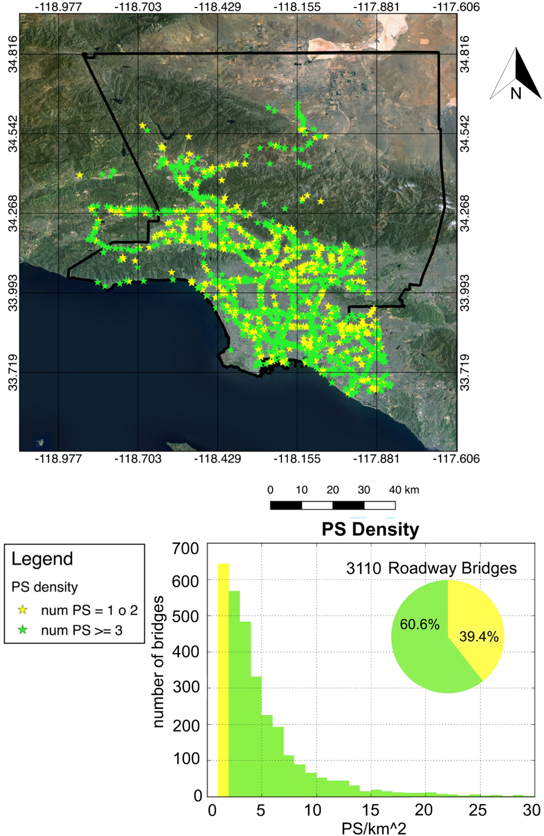

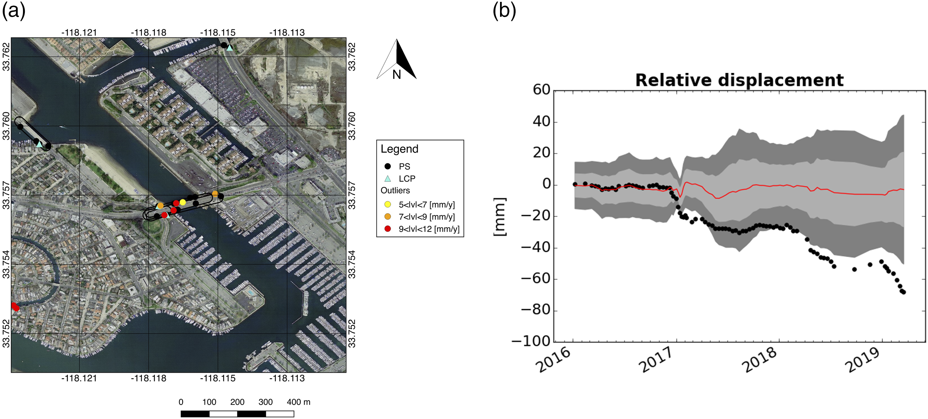
Figure 16 shows the distribution of the local deformation velocities and highlights the bridges deforming at a rate higher than 2 mm/year. The analysis led to the identification of 5374 outliers over the Los Angeles bridges, and showed that 1375 assets are characterised by at least 3 scatterers and have a local deformation velocity higher than 2 mm/year. Figure 17 shows a Los Angeles bridge for which outliers were detected, with a focus on the displacement-temporal series of the fastest moving point (Figure 17(b)).

Figure 16.

Average velocities relative to LCPs for the Los Angeles roadway bridges based on Sentinel data from 2016 to 2019. The proposed classification is based on relative velocity absolute values. Each asset is identified by a star symbol.

Figure 17.

Example of bridge with outliers in Los Angeles. (a) Aerial view of the bridge showing the scatterers producing an anomalous behaviour: red, orange and yellow scatterers correspond to the outliers retrieved on the asset, the Local Control Point (LCP) is indicated in light blue and the other PSs in black. (b) Relative displacement time-series of the fastest point with respect to the LCP: the red line refers to the average displacement time-series, obtained as the mean of the displacement time-series of all the PSs on the bridge. The light and dark grey bands indicate one (σ) and two (2σ) standard deviations from the average displacement time-series, respectively.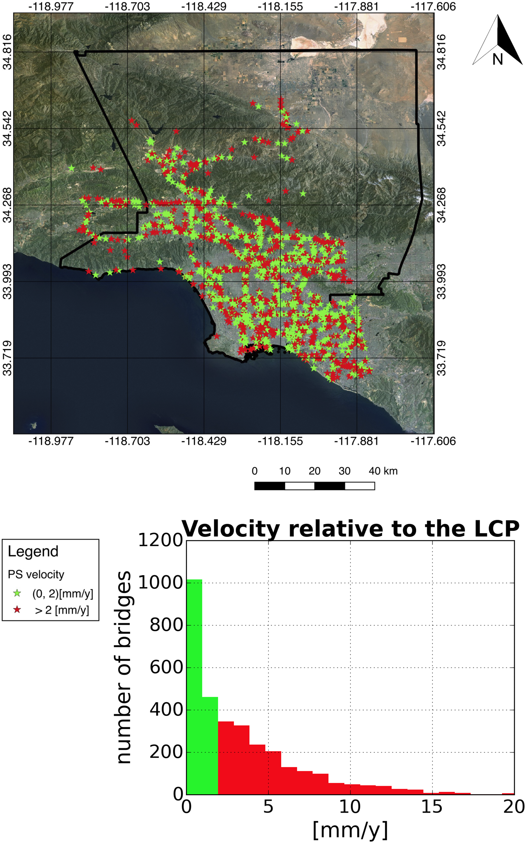

Validation case study: the Himera viaduct

To highlight how the proposed methodology contributes to infrastructure risk management, a case study for which the identified anomalies were associated with actual recorded damage is presented.

The Himera viaduct is a 2360-m-long reinforced concrete asset located on the A19 Palermo-Catania motorway between the municipalities of Scillato and Caltavuturo in the Sicily region, Italy. On 10 April 2015, the Himera viaduct was overrun by a landslide that caused a partial collapse of the asset. During the landslide, four viaduct piers were damaged, with one of them experiencing tilt. This resulted in both shift and subsidence of the viaduct deck. After the hazardous event, that stretch of motorway was closed, causing enormous economic losses to the Region and several logistic issues to inhabitants.

The Himera viaduct is located along a region of the Imera river basin, where the combination of tectonic activities and hydrological and geomorphological conditions have led to the occurrence of several landslide events over recent years.¹⁵³ In Rocca di Sciara, which is a slope adjacent to the Himera viaduct, intense landslide activities have been observed since 2005, when a vast portion of the nearby provincial road SP24 was damaged. The landslide that damaged the Himera viaduct in 2015 was likely triggered by heavy rainfalls which occurred over the months prior to failure.¹⁵⁴ The landslide involved a portion of the slope located between 380 m and 230 m a.s.l., and developed in Numidian Flysch deposits, which mainly consist of clay materials. At the time of the viaduct failure, the landslide was 600-m-long and 290-m-wide, with the sliding body reaching a presumed depth of 15–20 m. As the landslide exhibited both rotational and translational movements, it was classified as complex, according to the definition proposed by Varnes.¹⁵⁵

Analysis of the COSMO-SkyMed data resulted in the identification of 17 outliers on the Himera viaduct: 5 from ascending and 12 from descending acquisition geometries. These outliers were analysed in relation to landslides catalogues and PSs located on the slopes adjacent to the asset. Figure 18 shows the distribution of ascending and descending PS velocities, outliers and LCPs for the analysed area. Landslides are also indicated and classified according to their movement type. The area located south of the viaduct corresponds to Rocca di Sciara. The region delimited by a purple dashed line is affected by a deep-seated gravitational slope deformation (DGSD), which is an ancient gravitational-induced process typically evolving over years. The landslides within this area, which also include the 2015 landslide, form a complex system of spatially and temporally connected landslides, and their interactions and evolutions can contribute to reactivation scenarios.¹⁵³

Figure 18.

View of the landslide system and COSMO-SkyMed data over the Himera viaduct and the adjacent Rocca di Sciara, with PS velocities captured from (a) ascending and (b) descending acquisition geometries, respectively. Each dot indicates a PS whose colour represents its LOS deformation rate between 2011 and 2014. The LCPs and outliers are also shown in the maps. The dashed purple line identifies a region in Rocca di Sciara affected by deep-seated gravitational slope deformation (DGSD). The landslides are classified according to the type of movement. In each map, the arrow indicates the outlier for which the displacement-temporal series with respect to the corresponding LCP is shown in Figure 19.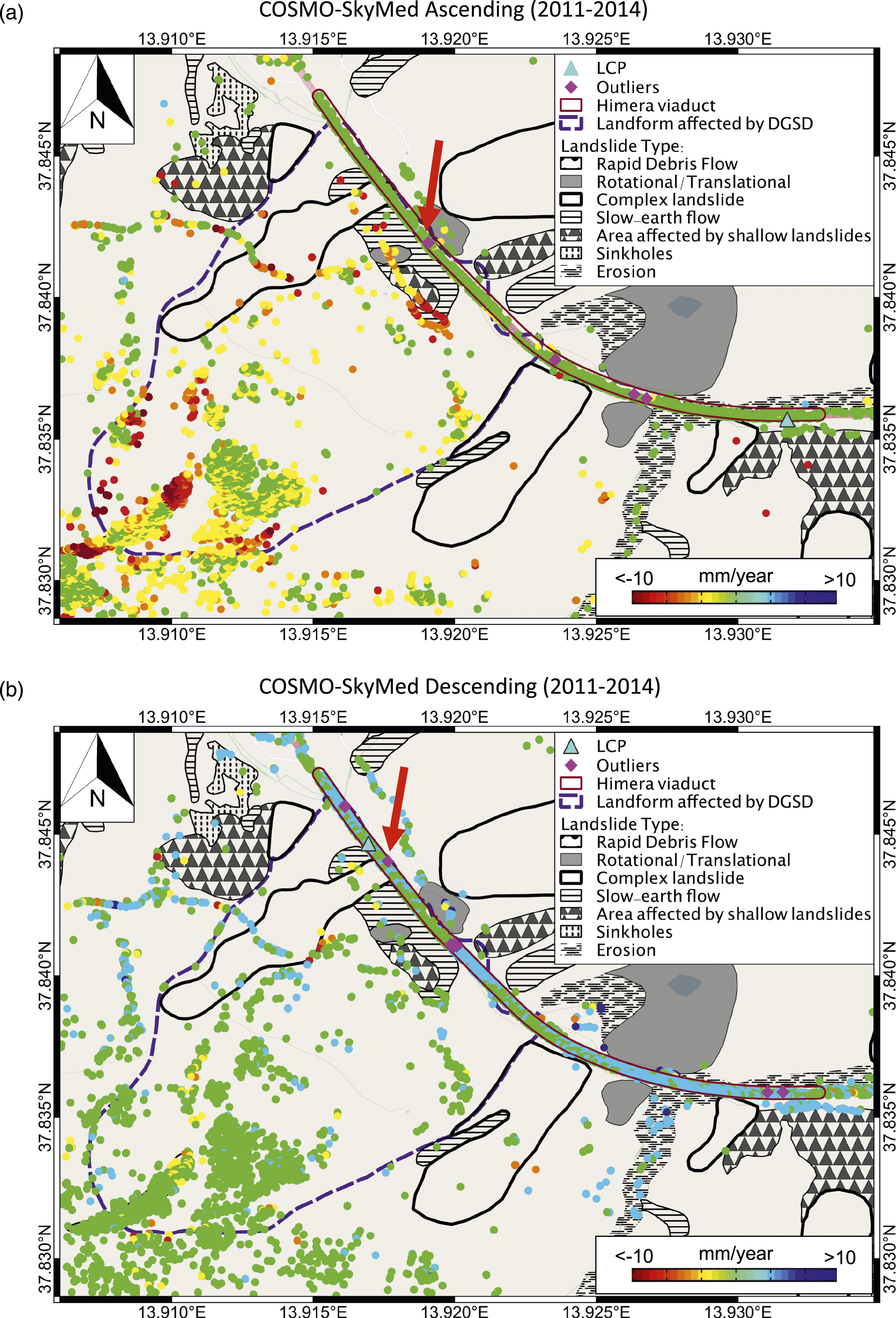

The COSMO-SkyMed data show that in Rocca di Sciara landslide activities were already ongoing between 2011 and 2014. This is more evident in the ascending acquisition geometry (Figure 18(a)), where several PSs with LOS velocities lower than −6 mm/year were found in the area near to the Himera viaduct. These PSs mainly belong to the provincial road SP24 that after being damaged during the 2005 landslide was damaged again in 2015.

The ascending and descending datasets led to the identification of 966 and 1346 PSs on the Himera viaduct, respectively. While most of the PSs were characterised by a stable velocity with respect to the respective LCP, outliers were identified for both ascending and descending datasets. Figure 19 shows the time-series of relative displacements of two outliers captured from ascending and descending acquisition geometries, respectively. Such outliers are located nearby the portion of the viaduct that was damaged several months later, and may indicate a preliminary sign of transient deformations or a distress condition of the structure.

Figure 19.

Relative displacement time-series with respect to LCPs of anomalous points on the Himera viaduct, captured from (a) ascending and (b) descending acquisition geometries, respectively. The time-series in (a) and (b) corresponds to the outliers indicated by the arrows in Figures 18(a) and (b), respectively. The red line refers to the average displacement time-series, obtained as the mean of the displacement time-series of the PSs on the bridge. The light and dark grey bands indicate one (σ) and two (2σ) standard deviations from the average displacement time-series, respectively. The displacement rate v indicates the absolute value of velocity relative to the corresponding LCP, and corresponds to the slope of the black line. The dashed blue line and blue triangle indicate the dates from which the relative deformation time-series exceed 2σ.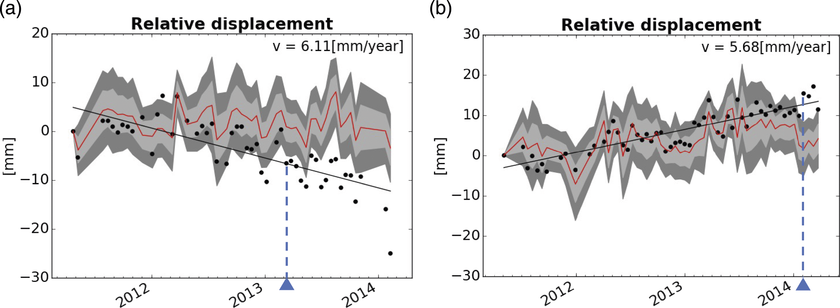

Discussion

The use of ERS/Envisat, COSMO-SkyMed and Sentinel MT-InSAR datasets for two different case studies showed the flexibility of the proposed methodology for the monitoring of different infrastructure networks, using input datasets with different resolutions, extent and characteristics. ERS/Envisat historical data cover all the Italian motorway network and can be used for detecting pre-existing long-term structural trends. Thanks to COSMO-SkyMed better spatial resolution (Range × Azimuth resolutions are 3 m × 3 m for COSMO-SkyMed, 6 m × 24 m for ERS/Envisat, and 5 m × 20 m for Sentinel-1), the average number of PSs per km² of infrastructure typically available with ERS/Envisat or Sentinel can increase by a factor of 23 when COSMO-SkyMed is used. Furthermore, COSMO-SkyMed data can guarantee a better geolocalization of the scatterers. Sentinel data can provide a factor of 1.2 more PSs per km² of infrastructure than ERS/Envisat, and deformation trends can be reconstructed with a rate three times higher than COSMO-SkyMed (6 days orbit repeat for Sentinel, and 16 days for COSMO-SkyMed), with the possibility to identify anomalous behaviours in near-real time.

As open-source processed MT-InSAR datasets are becoming more available,^64,133 PS density information is useful to evaluate which parts of a given network can be monitored through an accessible dataset. In contrast to in-situ monitoring instruments which provide measurements for controlled sparse points located on a given structure, the location of PSs is not known before completion of MT-InSAR analysis, with MT-InSAR measurements often available with uneven distribution. As the reliability of results is sensitive to the number of PSs per structure and to the spatial distribution of these points along the structure, PS density maps can be used to support interpretation of results. If only 1 PS is obtained on an asset, geological instabilities and seasonal trends cannot be removed and relative movements within the structure cannot be estimated. Consequently, the identification of deformation trends along the structure is not feasible. Even if 2 PSs are retrieved, the observation of deformation phenomena is still difficult. However, the exploitation of both ascending and descending orbits and different satellite datasets can provide a higher PS density, increasing the reliability of results.

The accuracy of results depends also on the accuracy of the infrastructure catalogue used as an input. In some cases, multiple occurrences of the same asset were listed in the analysed infrastructure catalogue. In addition, some assets are missing in the database. Infrastructure catalogues with higher precision would guarantee more accurate results.

The deformation time-series obtained during MT-InSAR analysis are determined with respect to a GCP. Consequently, the identification of a stable point on the structure, i.e., the LCP, is essential to remove geological instabilities, seasonal effects and possible noise caused by the use of a distant GCP during MT-InSAR analysis. This allows the observation of the displacement field of the structure alone, highlighting the possible presence of anomalous relative movements within the structure. However, in presence of a low number of PSs or inhomogeneous geological instabilities below the asset, it is less likely that a reliable reference point on the structure will be identified. The use of multiple GCPs during the processing would help to remove local instabilities, reducing the dependence of the result on the LCP.

Finally, this methodology can be used to screen large networks and identify the infrastructure regions that require an in-depth investigation. As shown through the case of the Himera viaduct in Italy, the proposed methodology enables the identification of critical areas, where the presence of outliers could initiate geotechnical evaluations and in-situ monitoring campaigns aimed to interpret the cause of the anomalies and asses the health of the structure. It is remarked that the presence of anomalous trends is not a straightforward indicator of a severe structural condition, but highlights an unusual behaviour that should be investigated more in depth. It is important to underline that the effect of the detected movements can only be determined by integrating structural analysis and the observed deformations. For example, for some types of bridges, the occurrence of settlement does not necessarily produce damage into the structure.⁹⁰ A future integration of the displacement information with the geometry and the construction material of the specific asset would enable a more accurate evaluation of the structural conditions, with the possibility to develop a statistical characterisation of structural deformation processes on a regional scale.

Conclusions

This study investigates the use of MT-InSAR techniques for monitoring critical infrastructure networks and presents an automated methodology for obtaining surface displacement data over large infrastructure systems. These data could be used to assess the deformation of assets over time or incorporated into an early warning system to aid transport network managers. A fully automated and multi-step methodology integrating MT-InSAR data and GIS-based infrastructure catalogues was developed. The designed methodology allows the density of monitoring points to be assessed and enables retrieval of average displacements, velocities and potential anomalies along segments of linear infrastructure. Maps showing the distribution of these indicators and critical locations are the output of the proposed methodology. In addition, an improved version of the traditional PSI processing chain was presented.

The capability of the proposed methodology was demonstrated through application to two case studies, showing that it is not restricted to a specific input dataset, but could be used for any national or regional analysis of transport infrastructure networks for which processed InSAR deformation measurements are available. The Los Angeles freeway and highway network was analysed using a Sentinel dataset from 2016 to 2019. The dataset consists of 84 SAR images processed using the SARPROZ software tool. The Italian motorway network was analysed using open access PS-datasets from different InSAR sensors. Specifically, 589 ERS/Envisat PS-datasets between 1992 and 2010, 120 COSMO-SkyMed PS-datasets between 2008 and 2014, and seven Sentinel PS-datasets between 2014 and 2020 were used. The Italian datasets include both ascending and descending acquisition geometries. The Sentinel dataset provided 10,117 PSs and about 1 million displacement measurements over the Los Angeles highway and freeway network, accounting for an average of 326 PS per km² of infrastructure. On the Italian motorway network, the ERS/Envisat datasets provided over 286,000 PSs and 14 million displacement measurements, corresponding to an average of 364 PS per km² of infrastructure. About 1.5 million PSs and 69 million displacement measurements were identified using the COSMO-SkyMed datasets, accounting for an average of 8400 PS per km² of infrastructure. The Sentinel datasets in Tuscany, Italy, provided 11,276 PSs and about 3 million displacement measurements on the motorway network, corresponding to an average of 417 PS per km² of infrastructure. To show the flexibility of the proposed methodology to the analysis of different infrastructure classes, the Sentinel dataset over Los Angeles County was used to analyse Los Angeles roadway bridges. Finally, to show the capability of the proposed methodology to forewarn potentially damaging movements, the case of an Italian motorway viaduct that had been damaged in 2015 was presented.

The following conclusions can be drawn:

• the proposed methodology enables the automated monitoring of critical infrastructure networks, allowing the displacement field and deformation velocities over large infrastructure systems to be extracted;

• the proposed methodology enables the identification and mapping of infrastructure segments and assets with higher local deformation rates and/or points moving much faster than other parts of the structure (LCP), and that may be related to anomalous structural behaviours;

• the proposed methodology enables the comparison of the performance of different satellite datasets for infrastructure monitoring, allowing the quality of monitoring over different parts of a given network and different infrastructure assets to be assessed;

• the application of the developed method to roadway networks and bridges shows that it can be used on linear infrastructure or individual assets, highlighting its potential for the structural assessment of different infrastructure typologies;

• its application to case studies with a different spatial extent shows how the proposed methodology can be used from city to national scale.

The proposed methodology has the potential to be integrated into traditional structural health monitoring systems and complement ground-based monitoring solutions. The identification of deformation trends highlights the possibility for this method to be used to support inspection planning. As an example, if anomalous behaviours are detected in the time lapse between two consecutive inspections, the developed tool could be used to reschedule the inspection timeline for the specific asset. In addition, giving an indication of the quality of the monitoring, the proposed methodology can support decisions about the selection of InSAR datasets for a specific test area, emphasising situations in which multiple datasets are essential to guarantee satisfactory coverage. Finally, a future integration with structural models would offer the potential to investigate the structural conditions of the monitored assets, providing an assessment tool for large transport systems.

Footnotes

Acknowledgements

We thank the European Space Agency for providing Sentinel data over Los Angeles for this project. COSMO-SkyMed and ERS/Envisat InSAR time-series were provided by the Italian Ministry of the Environment through the Geoportale Nazionale database (http://www.pcn.minambiente.it/mattm/). Sentinel InSAR time-series over Tuscany were accessed on 1 June 2020 through the Geoportale Regione Toscana (). Landslide shapefile data were provided by ISPRA License: CC BY SA 4.0. V. Macchiarulo was supported by a PhD scholarship granted by Sue and Roger Whorrod and the Alumni programme of the University of Bath. Part of this research was carried out when P. Milillo was at the Jet Propulsion Laboratory, California Institute of Technology, under a contract with the National Aeronautics and Space Administration.

Declaration of conflicting interests

The author(s) declared no potential conflicts of interest with respect to the research, authorship, and/or publication of this article.

Funding

The author(s) received no financial support for the research, authorship, and/or publication of this article.

ORCID iD

Valentina Macchiarulo

References

Jacobs

. Seven of the deadliest infrastructure failures throughout history. The New York Times, 2018.

Seattle . Infratructure Failures - Seattle Hazard Identification and Vulnerability Analysis.City of Seattle: Office of Emergency Management, 2014.

Marcuson

WFI

. Fixing America’s crumbling infrastructure: a call to action for all. Public Work Manag Policy 2008; 12(3): 473–475. DOI: 10.1177/1087724X07312145.

Lange

. The relevance of aging for civil infrastructure: the profession, the politics, the classroom. In: 1st international conference on ageing of materials & structures, pp. 17–25. DOI: 10.1007/978-3-319-70194-3_5.

Mehta

Burrows

. Building durable structures in the 21st century. Indian Concrete J 2001; 75(7): 437–443.

ARTBA . 2019 Bridge Report. Technical Report. The American Road & Transportation Builders Association, 2019.

ASCE . Infrastructure Report Card. Technical Report. ASCE (American Society of Civil Engineers) Foundation, 2017.

Pregnolato

. Bridge safety is not for granted – A novel approach to bridge management. Eng Struct 2019; 196: 109193. DOI: 10.1016/j.engstruct.2019.05.035.

Van Breugel

. Ageing infrastructure and circular economy: challenges and risks. In: Proceedings of the 2nd world congress on civil, structural, and environmental engineering (CSEE’17). DOI: 10.11159/icesdp17.1.

10.

Federal Ministry of Transport and Digital Infrastructure . Infrastructure as a Foundation for Growth, Jobs and Prosperity, 2018, https://www.bmvi.de/SharedDocs/EN/Dossier/infrastructure/2030-federal-transport-infrastructure-plan.html.

11.

Briginshaw

. Italy approves €28bn infrastructure investment hike. Int Railway J 2019.

12.

IPA . National Infrastructure Delivery Plan 2016–2021. Technical Report. Infrastructure and Projects Authority, 2016.

13.

Phares

Rolander

Graybeal

, et al. Reliability of visual bridge inspection. Public Roads 2001; 64(5).

14.

Stiros

Psimoulis

. Response of a historical short-span railway bridge to passing trains: 3-D deflections and dominant frequencies derived from Robotic Total Station (RTS) measurements. Eng Struct 2012; 45: 362–371. DOI: 10.1016/j.engstruct.2012.06.029.

15.

Cusson

Ghuman

Gara

, et al. Remote monitoring of bridges from space. Anais do 54° Congresso Brasileiro do Concreto - CBC2012 2012; 54: 1–25.

16.

DePrekel

Bouali

Oommen

. Monitoring the impact of groundwater pumping on infrastructure using Geographic Information System (GIS) and Persistent Scatterer Interferometry (PSI). Infrastructures 2018; 3(4): 57. DOI: 10.3390/infrastructures3040057.

17.

Sousa

Bastos

. Multi-temporal SAR interferometry reveals acceleration of bridge sinking before collapse. Nat Hazards Earth Syst Sci 2013; 13(3): 659–667. DOI: 10.5194/nhess-13-659-2013.

18.

Sousa

Hlaváčová

Bakoň

, et al. Potential of multi-temporal InSAR techniques for bridges and dams monitoring. Proc Technol 2014; 16: 834–841. DOI: 10.1016/j.protcy.2014.10.033.

19.

FHWA . National Bridge Inspection Standards, https://www.fhwa.dot.gov/bridge/nbis/(2018.

20.

Hearn

. Bridge inspection practices, volume 375. Transportation Research Board, 2007.

21.

Willsher

Tondo

Henley

. Bridges across Europe are in a dangerous state, warn experts. The Guardian, 2018.

22.

Pérez-Peña

. After Italy collapse, Europe asks: How safe are our bridges? The New York Times, 2018.

23.

Colesanti

Ferretti

Novali

, et al. SAR monitoring of progressive and seasonal ground deformation using the permanent scatterers technique. IEEE Trans Geosci Remote Sens 2003; 41(7): 1685–1701. DOI: 10.1109/TGRS.2003.813278.

24.

Ferretti

Prati

Rocca

. Nonlinear subsidence rate estimation using permanent scatterers in differential SAR interferometry. IEEE Trans Geosci Remote Sens 2000; 38: 2202–2212. DOI: 10.1109/36.868878.

25.

Ferretti

Prati

Rocca

. Permanent scatterers in SAR interferometry. IEEE Trans Geosci Remote Sens 2001; 39(1): 8–20. DOI: 10.1109/36.898661.

26.

Milillo

Riel

Minchew

, et al. On the synergistic use of SAR constellations’ data exploitation for earth science and natural hazard response. IEEE J Sel Top Appl Earth Obs Remote Sens 2015; 9(3): 1095–1100. DOI: 10.1109/JSTARS.2015.2465166.

27.

Ferretti

Savio

Barzaghi

, et al. Submillimeter accuracy of InSAR time series: experimental validation. IEEE Trans Geosci Remote Sens 2007; 45(5): 1142–1153. DOI: 10.1109/TGRS.2007.894440.

28.

Fornaro

Reale

Verde

. Bridge thermal dilation monitoring with millimeter sensitivity via multidimensional SAR imaging. IEEE Geosci Remote Sens Lett 2013; 10(4): 677–681. DOI: 10.1109/LGRS.2012.2218214.

29.

Chang

Hanssen

. Near real-time, semi-recursive, deformation monitoring of infrastructure using satellite radar interferometry. 2012 IEEE International Geoscience and Remote Sensing Symposium. IEEE, pp. 1876–1879. DOI: 10.1109/IGARSS.2012.6351141.

30.

Milillo

Giardina

DeJong

, et al. Multi-temporal InSAR structural damage assessment: the London crossrail case study. Remote Sens 2018; 10(2): 287. DOI: 10.3390/rs10020287.

31.

Tapete

Fanti

Cecchi

, et al. Satellite radar interferometry for monitoring and early-stage warning of structural instability in archaeological sites. J Geophys Eng 2012; 9(4): S10. DOI: 10.1088/1742-2132/9/4/S10.

32.

Chang

Hanssen

. A probabilistic approach for InSAR time-series postprocessing. IEEE Trans Geosci Remote Sens 2015; 54(1): 421–430. DOI: 10.1109/TGRS.2015.2459037.

33.

Chen

Lin

, et al. Interaction between permafrost and infrastructure along the Qinghai–Tibet Railway detected via jointly analysis of C-and L-band small baseline SAR interferometry. Remote Sens Environ 2012; 123: 532–540. DOI: 10.1016/j.rse.2012.04.020.

34.

Liu

Jia

Zhang

, et al. Exploration of subsidence estimation by persistent scatterer InSAR on time series of high resolution TerraSAR-X images. IEEE J Sel Top Appl Earth Obs Remote Sens 2010; 4(1): 159–170. DOI: 10.1109/JSTARS.2010.2067446.

35.

Bianchini

Pratesi

Nolesini

, et al. Building deformation assessment by means of persistent scatterer interferometry analysis on a landslide-affected area: the Volterra (Italy) case study. Remote Sens 2015; 7(4): 4678–4701. DOI: 10.3390/rs70404678.

36.

Cerchiello

Tessari

Velterop

, et al. Building damage risk by modeling interferometric time series. IEEE Geosci Remote Sens Lett 2017; 14(4): 509–513. DOI: 10.1109/LGRS.2017.2651938.

37.

Cigna

Lasaponara

Masini

, et al. Persistent scatterer interferometry processing of COSMO-SkyMed StripMap HIMAGE time series to depict deformation of the historic centre of Rome, Italy. Remote Sens 2014; 6(12): 12593–12618. DOI: 10.3390/rs61212593.

38.

Giardina

Milillo

DeJong

, et al. Evaluation of InSAR monitoring data for post-tunnelling settlement damage assessment. Struct Control Health Monit 2019; 26(2): e2285. DOI: 10.1002/stc.2285.

39.

Macchiarulo

Milillo

DeJong

, et al. Integrated InSAR monitoring and structural assessment of tunnelling-induced building deformations. Struct Control Health Monit 2021: e2781doi. DOI: 10.1002/stc.2781.

40.

Peduto

Nicodemo

Maccabiani

, et al. Multi-scale analysis of settlement-induced building damage using damage surveys and DInSAR data: a case study in the Netherlands. Eng Geol 2017; 218: 117–133. DOI: 10.1016/j.enggeo.2016.12.018.

41.

Peduto

Nicodemo

Caraffa

, et al. Quantitative analysis of consequences to masonry buildings interacting with slow-moving landslide mechanisms: a case study. Landslides 2018; 15(10): 2017–2030. DOI: 10.1007/s10346-018-1014-0.

42.

Peduto

Korff

Nicodemo

, et al. Empirical fragility curves for settlement-affected buildings: analysis of different intensity parameters for seven hundred masonry buildings in the Netherlands. Soils and Foundations 2019; 59(2): 380–397. DOI: 10.1016/j.sandf.2018.12.009.

43.

Shimoni

Lopez

Walstra

, et al. GEPATAR: a geotechnical based PS-InSAR toolbox for architectural conservation in Belgium. 2017 IEEE International Geoscience and Remote Sensing Symposium (IGARSS). IEEE, pp. 5555–5558. DOI: 10.1109/IGARSS.2017.8128263.

44.

Zhu

Wan

Fei

, et al. Detection of building and infrastructure instabilities by automatic spatiotemporal analysis of satellite SAR interferometry measurements. Remote Sens 2018; 10(11): 1816. DOI: 10.3390/rs10111816.

45.

Milillo

Giardina

Perissin

, et al. Pre-collapse space geodetic observations of critical infrastructure: the Morandi Bridge, Genoa, Italy. Remote Sens 2019; 11(12): 1403. DOI: 10.3390/rs11121403.

46.

Peduto

Giangreco

Venmans

. Differential settlements affecting transition zones between bridges and road embankments on soft soils: numerical analysis of maintenance scenarios by multi-source monitoring data assimilation. Transp Geotech 2020; 24: 100369. DOI: 10.1016/j.trgeo.2020.100369.

47.

Carlá

Intrieri

Raspini

, et al. Perspectives on the prediction of catastrophic slope failures from satellite InSAR. Sci Rep 2019; 9(1): 1–9. DOI: 10.1038/s41598-019-50792-y.

48.

Lazeckỳ

Perissin

Zhiying

, et al. Observing dam’s movements with spaceborne SAR interferometry. In: Engineering Geology for Society and Territory-Volume 5. Springer; 2015, pp. 131–136. DOI: 10.1007/978-3-319-09048-1_26.

49.

Milillo

Bürgmann

Lundgren

, et al. Space geodetic monitoring of engineered structures: the ongoing destabilization of the Mosul dam, Iraq. Sci Rep 2016; 6: 37408. DOI: 10.1038/srep37408.

50.

Milillo

Perissin

Salzer

, et al. Monitoring dam structural health from space: insights from novel InSAR techniques and multi-parametric modeling applied to the Pertusillo dam Basilicata, Italy. Int J Appl Earth Obs Geoinf 2016; 52: 221–229. DOI: 10.1016/j.jag.2016.06.013.

51.

Chang

Dollevoet

Hanssen

. Nationwide railway monitoring using satellite SAR interferometry. IEEE J Sel Top Appl Earth Obs Remote Sens 2016; 10(2): 596–604. DOI: 10.1109/JSTARS.2016.2584783.

52.

Bianchini Ciampoli

Gagliardi

Clementini

, et al. Transport infrastructure monitoring by InSAR and GPR data fusion. Surv Geophys 2019: 1–24. DOI: 10.1007/s10712-019-09563-7.

53.

North

Farewell

Hallett

, et al. Monitoring the response of roads and railways to seasonal soil movement with Persistent Scatterers Interferometry over six UK sites. Remote Sens 2017; 9(9): 922. DOI: 10.3390/rs9090922.

54.

Peduto

Huber

Speranza

, et al. DInSAR data assimilation for settlement prediction: case study of a railway embankment in the Netherlands. Can Geotech J 2017; 54(4): 502–517. DOI: 10.1139/cgj-2016-0425.

55.

Bruno

Molfetta

Mossa

, et al. Integration of multitemporal SAR/InSAR techniques and NWM for coastal structures monitoring: outline of the software system and of an operational service with COSMO-SkyMed data. 2016 IEEE Workshop on Environmental, Energy, and Structural Monitoring Systems (EESMS). IEEE, pp. 1–6. DOI: 10.1109/EESMS.2016.7504837.

56.

Delgado Blasco

Foumelis

Stewart

, et al. Measuring urban subsidence in the Rome Metropolitan Area (Italy) with Sentinel-1 SNAP-StaMPS persistent scatterer interferometry. Remote Sens 2019; 11(2): 129. DOI: 10.3390/rs11020129.

57.

Infante

Di Martire

Calcaterra

, et al. Integrated Procedure for Monitoring and Assessment of Linear Infrastructures Safety (I-Pro MONALISA) affected by slope instability. Appl Sci 2019; 9(24): 5535. DOI: 10.3390/app9245535.

58.

Nappo

Peduto

Mavrouli

, et al. Slow-moving landslides interacting with the road network: analysis of damage using ancillary data, in situ surveys and multi-source monitoring data. Eng Geol 2019; 260: 105244. DOI: 10.1016/j.enggeo.2019.105244.

59.

Wasowski

Bovenga

Nutricato

, et al. High resolution satellite multi-temporal interferometry for monitoring infrastructure instability hazards. Innov Infrastruct Solut 2017; 2(1): 27. DOI: 10.1007/s41062-017-0077-4.

60.

Bianchini Ciampoli

Gagliardi

Calvi

, et al. Automatic network level bridge monitoring by integration of InSAR and GIS catalogues. In: Multimodal Sensing: Technologies and Applications, volume 11059. International Society for Optics and Photonics, p. 110590I.

61.

Bordoni

Bonì

Colombo

, et al. A methodology for ground motion area detection (GMA-D) using A-DInSAR time series in landslide investigations. Catena 2018; 163: 89–110. DOI: 10.1016/j.catena.2017.12.013.

62.

Meisina

Zucca

Notti

, et al. Geological interpretation of PSInSAR data at regional scale. Sensors 2008; 8(11): 7469–7492. DOI: 10.3390/s8117469.

63.

Peduto

Cascini

Arena

, et al. A general framework and related procedures for multiscale analyses of DInSAR data in subsiding urban areas. ISPRS J Photogramm Remote Sens 2015; 105: 186–210. DOI: 10.1016/j.isprsjprs.2015.04.001.

64.

Raspini

Bianchini

Ciampalini

, et al. Continuous, semi-automatic monitoring of ground deformation using Sentinel-1 satellites. Sci Rep 2018; 8(1): 1–11. DOI: 10.1038/s41598-018-25369-w.

65.

Bamler

Hartl

. Synthetic aperture radar interferometry. Inverse Probl 1998; 14(4): R1.

66.

Rosen

Hensley

Joughin

, et al. Synthetic aperture radar interferometry. Proc IEEE 2000; 88(3): 333–382. DOI: 10.1109/5.838084.

67.

Crosetto

Crippa

Biescas

, et al. State of the art of land deformation monitoring using differential SAR interferometry. In: ISPRS Hannover Workshop, pp. 17–20.

68.

Berardino

Fornaro

Lanari

, et al. A new algorithm for surface deformation monitoring based on small baseline differential SAR interferograms. IEEE Trans Geosci Remote Sens 2002; 40(11): 2375–2383. DOI: 10.1109/TGRS.2002.803792.

69.

Lanari

Mora

Manunta

, et al. A small-baseline approach for investigating deformations on full-resolution differential SAR interferograms. IEEE Trans Geosci Remote Sens 2004; 42(7): 1377–1386. DOI: 10.1109/TGRS.2004.828196.

70.

Cavalagli

Kita

Falco

, et al. Satellite radar interferometry and in-situ measurements for static monitoring of historical monuments: the case of Gubbio, Italy. Remote Sens Environ 2019; 235: 111453. DOI: 10.1016/j.rse.2019.111453.

71.

Gantert

Kern

Düring

, et al. The future of X-band SAR: TerraSAR-X next generation and WorldSAR constellation. In: Conference Proceedings of 2013 Asia-Pacific Conference on Synthetic Aperture Radar (APSAR). IEEE, pp. 20–23.

72.

Geudtner

Torres

Snoeij

, et al. Sentinel-1 system capabilities and applications. In 2014 IEEE Geoscience and Remote Sensing Symposium. IEEE, pp. 1457–1460. DOI: 10.1109/IGARSS.2014.6946711.

73.

Potin

Bargellini

Laur

, et al. Sentinel-1 mission operations concept. In 2012 IEEE International Geoscience and Remote Sensing Symposium. IEEE, pp. 1745–1748. DOI: 10.1109/IGARSS.2012.6351183.

74.

Bonano

Manunta

Pepe

, et al. From previous C-band to new X-band SAR systems: assessment of the DInSAR mapping improvement for deformation time-series retrieval in urban areas. IEEE Trans Geosci Remote Sens 2013; 51(4): 1973–1984. DOI: 10.1109/TGRS.2012.2232933.

75.

Crosetto

Monserrat

Iglesias

, et al. Persistent scatterer interferometry. Photogramm Eng Remote Sens 2010; 76(9): 1061–1069. DOI: 10.14358/PERS.76.9.1061.

76.

Franceschetti

Iodice

Riccio

. A canonical problem in electromagnetic backscattering from buildings. IEEE Trans Geosci Remote Sens 2002; 40(8): 1787–1801. DOI: 10.1109/TGRS.2002.802459.

77.

Perissin

Ferretti

. Urban-target recognition by means of repeated spaceborne SAR images. IEEE Trans Geosci Remote Sens 2007; 45(12): 4043–4058. DOI: 10.1109/TGRS.2007.906092.

78.

Drougkas

Verstrynge

Van Balen

, et al. Country-scale InSAR monitoring for settlement and uplift damage calculation in architectural heritage structures. Struct Health Monit 2020: 1475921720942120. DOI: 10.1177/1475921720942120.

79.

Perski

van Leijen

Hanssen

. Applicability of PSInSAR for building hazard identification. Study of the 29 January 2006 Katowice exhibition hall collapse and the 24 February 2006 Moscow basmanny market collapse. In: ESA ENVISAT Symposium. Switzerland: MontreuxApril, pp. 23–27.

80.

Chang

Dollevoet

RPBJ

Hanssen

. Railway infrastructure monitoring using satellite radar data. Int J Railway Technol 2014; 3: 79–91. DOI: 10.4203/ijrt.3.2.5.

81.

Wang

Zhang

, et al. Seasonal deformation features on Qinghai-Tibet railway observed using time-series InSAR technique with high-resolution TerraSAR-X images. Remote Sens Lett 2017; 8(1): 1–10. DOI: 10.1080/2150704X.2016.1225170.

82.

Luo

Perissin

Lin

, et al. Subsidence monitoring of Tianjin suburbs by TerraSAR-X persistent scatterers interferometry. IEEE J Sel Top Appl Earth Obs Remote Sens 2013; 7(5): 1642–1650. DOI: 10.1109/JSTARS.2013.2271501.

83.

Vaccari

Batabyal

Tabassum

, et al. Integrating remote sensing data in decision support systems for transportation asset management. Transp Res Rec 2018; 2672(45): 23–35. DOI: 10.1177/0361198118786645.

84.

Samarelli

Agrimano

Epicoco

, et al. Rheticus®: a Cloud-Based Geo-Information Service for Ground Instabilities Detection and Monitoring. In: IGARSS 2018-2018 IEEE International Geoscience and Remote Sensing Symposium. IEEE, pp. 2238–2240. DOI: 10.1109/IGARSS.2018.8518226.

85.

Jones

Blom

, et al. Anthropogenic and geologic influences on subsidence in the vicinity of New Orleans, Louisiana. J Geophys Res Solid Earth 2016; 121(5): 3867–3887. DOI: 10.1002/2015JB012636.

86.

Nguyen

DDC

Bennett

O’Meara

. New Orleans levee displacement study via interferometric point target analysis technique and in situ instrumentation. J Geotech Geoenviron Eng 2019; 145(8): 04019032. DOI: 10.1061/(ASCE)GT.1943-5606.0002067.

87.

Del Soldato

Tomás

Pont Castillo

, et al. A multi-sensor approach for monitoring a road bridge in the Valencia harbor (SE Spain) by SAR Interferometry (InSAR). Rendiconti Online Della Società Gelogica Italiana 2016; 41: 235–238. DOI: 10.3301/ROL.2016.137.

88.

Huang

Monserrat

Crosetto

, et al. Displacement monitoring and health evaluation of two bridges using Sentinel-1 SAR images. Remote Sens 2018; 10(11): 1714. DOI: 10.3390/rs10111714.

89.

Lazeckỳ

Hlavacova

Bakon

, et al. Bridge displacements monitoring using space-borne X-band SAR interferometry. IEEE J Sel Top Appl Earth Obs Remote Sens 2016; 10(1): 205–210. DOI: 10.1109/JSTARS.2016.2587778.

90.

Peduto

Elia

Montuori

. Probabilistic analysis of settlement-induced damage to bridges in the city of Amsterdam (The Netherlands). Transp Geotech 2018; 14: 169–182. DOI: 10.1016/j.trgeo.2018.01.002.

91.

Selvakumaran

Rossi

Marinoni

, et al. Combined InSAR and terrestrial structural monitoring of bridges. IEEE Trans Geosci Remote Sens 2020; 216: 71–90. DOI: 10.1109/TGRS.2020.2979961.

92.

Zhao

Ding

, et al. Elevation extraction and deformation monitoring by multitemporal InSAR of Lupu Bridge in Shanghai. Remote Sens 2017; 9(9): 897. DOI: 10.3390/rs9090897.

93.

Tomás

Cano

Garcia-Barba

, et al. Monitoring an earthfill dam using differential SAR interferometry: La Pedrera dam, Alicante, Spain. Eng Geol 2013; 157: 21–32. DOI: 10.1016/j.enggeo.2013.01.022.

94.

Di Martire

Iglesias

Monells

, et al. Comparison between differential SAR interferometry and ground measurements data in the displacement monitoring of the earth-dam of Conza della Campania (Italy). Remote Sens Environ 2014; 148: 58–69. DOI: 10.1016/j.rse.2014.03.014.

95.

Colesanti

Mouelic

Bennani

, et al. Detection of mining related ground instabilities using the Permanent Scatterers technique – a case study in the east of France. Int J Remote Sens 2005; 26(1): 201–207. DOI: 10.1080/0143116042000274069.

96.

Raucoules

Bourgine

De Michele

, et al. Validation and intercomparison of Persistent Scatterers Interferometry: PSIC4 project results. J Appl Geophys 2009; 68(3): 335–347. DOI: 10.1016/j.jappgeo.2009.02.003.

97.

Bekaert

Hamlington

Buzzanga

, et al. Spaceborne synthetic aperture radar survey of subsidence in Hampton Roads, Virginia (USA). Sci Rep 2017; 7(1): 1–9. DOI: 10.1038/s41598-017-15309-5.

98.

Heleno

SIN

Oliveira

LGS

Henriques

, et al. Persistent scatterers interferometry detects and measures ground subsidence in Lisbon. Remote Sens Environ 2011; 115(8): 2152–2167. DOI: 10.1016/j.rse.2011.04.021.

99.

Khorrami

Alizadeh

Ghasemi Tousi

, et al. How groundwater level fluctuations and geotechnical properties lead to asymmetric subsidence: a PSInSAR analysis of land deformation over a transit corridor in the Los Angeles Metropolitan Area. Remote Sens 2019; 11(4): 377. DOI: 10.3390/rs11040377.

100.

Musson

RMW

Haynes

Ferretti

. Space-based tectonic modeling in subduction areas using PSInSAR. Seismol Res Lett 2004; 75(5): 598–606. DOI: 10.1785/gssrl.75.5.598.

101.

Perissin

Rocca

. High-accuracy urban DEM using permanent scatterers. IEEE Trans Geosci Remote Sens 2006; 44(11): 3338–3347. DOI: 10.1109/TGRS.2006.877754.

102.

Perissin

. Validation of the submetric accuracy of vertical positioning of PSs in C-band. IEEE Geosci Remote Sens Lett 2008; 5(3): 502–506. DOI: 10.1109/LGRS.2008.921210.

103.

Di Maio

Fornaro

Gioia

, et al. In situ and satellite long-term monitoring of the Latronico landslide, Italy: displacement evolution, damage to buildings, and effectiveness of remedial works. Eng Geol 2018; 245: 218–235. DOI: 10.1016/j.enggeo.2018.08.017.

104.

Luo

Zhou

Perissin

. Monitoring of subsidence along Jingjin inter-city railway with high-resolution TerraSAR-X MT-InSAR analysis. Remote Sens 2017; 9(7): 717. DOI: 10.3390/rs9070717.

105.

Peduto

Santoro

Aceto

, et al. Full integration of geomorphological, geotechnical, A-DInSAR and damage data for detailed geometric-kinematic features of a slow-moving landslide in urban area. Landslides 2021; 18(3): 807–825. DOI: 10.1007/s10346-020-01541-0.

106.

Wang

Chang

Markine

. Structural health monitoring of railway transition zones using satellite radar data. Sensors 2018; 18(2): 413. DOI: 10.3390/s18020413.

107.

Arangio

Calò

Di Mauro

, et al. An application of the SBAS-DInSAR technique for the assessment of structural damage in the city of Rome. Struct Infrastruct Eng 2014; 10(11): 1469–1483.

108.

Ferlisi

Marchese

Peduto

. Quantitative analysis of the risk to road networks exposed to slow-moving landslides: a case study in the Campania region (southern Italy). Landslides 2021; 18(1): 303–319. DOI: 10.1007/s10346-020-01482-8.

109.

Nappo

Peduto

Polcari

, et al. Subsidence in Como historic centre (northern Italy): assessment of building vulnerability combining hydrogeological and stratigraphic features, Cosmo-SkyMed InSAR and damage data. Int J Disaster Risk Reduct 2021; 56: 102115. DOI: 10.1016/j.ijdrr.2021.102115.

110.

Peduto

Ferlisi

Nicodemo

, et al. Empirical fragility and vulnerability curves for buildings exposed to slow-moving landslides at medium and large scales. Landslides 2017; 14(6): 1993–2007. DOI: 10.1007/s10346-017-0826-7.

111.

Huang

Crosetto

Monserrat

, et al. Displacement monitoring and modelling of a high-speed railway bridge using C-band Sentinel-1 data. ISPRS J Photogramm Remote Sens 2017; 128: 204–211. DOI: 10.1016/j.isprsjprs.2017.03.016.

112.

Cusson

Trischuk

Hébert

, et al. Satellite-based InSAR monitoring of highway bridges: validation case study on the North Channel Bridge in Ontario, Canada. Transp Res Rec 2018; 2672(45): 76–86.

113.

Qin

Zhang

Yang

, et al. Mapping surface deformation and thermal dilation of arch bridges by structure-driven multi-temporal DInSAR analysis. Remote Sens Environ 2018; 216: 71–90. DOI: 10.1016/j.rse.2018.06.032.

114.

Hoppe

Novali

Rucci

, et al. Deformation monitoring of posttensioned bridges using high-resolution satellite remote sensing. J Bridge Eng 2019; 24(12): 04019115. DOI: 10.1061/(ASCE)BE.1943-5592.0001479.

115.

Liu

Wang

, et al. Damage detection and analysis of urban bridges using terrestrial laser scanning (TLS), ground-based microwave interferometry, and permanent scatterer interferometry synthetic aperture radar (PS-InSAR). Remote Sens 2019; 11(5): 580. DOI: 10.3390/rs11050580.

116.

Fang

, et al. A tentative test for measuring the sub-millimeter settlement and uplift of a high-speed railway bridge using COSMO-SkyMed images. ISPRS J Photogramm Remote Sens 2019; 155: 1–12. DOI: 10.1016/j.isprsjprs.2019.06.013.

117.

Alani

Tosti

Bianchini Ciampoli

, et al. An integrated investigative approach in health monitoring of masonry arch bridges using GPR and InSAR technologies. NDT E Int 2020; 115: 102288DOI: 10.1016/j.ndteint.2020.102288.

118.

Grenerczy

Wegmüller

. Persistent scatterer interferometry analysis of the embankment failure of a red mud reservoir using ENVISAT ASAR data. Nat Hazards 2011; 59(2): 1047. DOI: 10.1007/s11069-011-9816-6.

119.

Wang

Perissin

Rocca

, et al. Three Gorges Dam stability monitoring with time-series InSAR image analysis. Sci China Earth Sci 2011; 54(5): 720–732. DOI: 10.1007/s11430-010-4101-1.

120.

Ruiz-Armenteros

Lazeckỳ

Hlaváčová

, et al. Deformation monitoring of dam infrastructures via spaceborne MT-InSAR. The case of La Viñuela (Málaga, southern Spain). Proc Comput Sci 2018; 138: 346–353. DOI: 10.1016/j.procs.2018.10.049.

121.

Wang

Huang

, et al. Displacement monitoring of upper Atbara dam based on time series InSAR. Surv Rev 2020; 52: 485–496. DOI: 10.1080/00396265.2019.1643529.

122.

AHM

, et al. Risk assessment for tailings dams in Brumadinho of Brazil using InSAR time series approach. Sci Total Environ 2020; 717: 137125. DOI: 10.1016/j.scitotenv.2020.137125.

123.

Chang

Hanssen

. Detection of permafrost sensitivity of the Qinghai–Tibet railway using satellite radar interferometry. Int J Remote Sens 2015; 36(3): 691–700. DOI: 10.1080/01431161.2014.999886.

124.

Poreh

Iodice

Riccio

, et al. Railways’ stability observed in Campania (Italy) by InSAR data. Eur J Remote Sens 2016; 49(1): 417–431. DOI: 10.5721/EuJRS20164923.

125.

Qin

Liao

Zhang

, et al. Structural health and stability assessment of high-speed railways via thermal dilation mapping with time-series InSAR analysis. IEEE J Sel Top Appl Earth Obs Remote Sens 2017; 10(6): 2999–3010. DOI: 10.1109/JSTARS.2017.2719025.

126.

Zhao

Chen

Gong

, et al. Land subsidence along the Beijing–Tianjin Intercity Railway during the period of the South-to-North Water Diversion Project. Int J Remote Sens 2020; 41(12): 4447–4469. DOI: 10.1080/01431161.2020.1718238.

127.

Lazeckỳ

Rapant

Perissin

, et al. Deformations of highway over undermined Ostrava-Svinov area monitored by InSAR using limited set of SAR images. Proc Technol 2014; 16: 414–421. DOI: 10.1016/j.protcy.2014.10.107.

128.

Infante

Di Martire

Confuorto

, et al. Differential sar interferometry technique for control of linear infrastructures affected by ground instability phenomena. Int Arch Photogramm, Remote Sens Spat Inf Sci 2018; 42(3/W4). DOI: 10.5194/isprs-archives-XLII-3-W4-251-2018.

129.

CAMS . Los Angeles County Countywide Address Management System. L.A. County Street & Address File, 2019, http://egis3.lacounty.gov/dataportal/2014/06/16/2011-la-county-street-centerline-street-address-file/.

130.

Geoportale Nazionale . National Geoportal of the Italian Ministry of Environment, 2019, http://www.pcn.minambiente.it/mattm/en/.

131.

132.

Perissin

Wang

. The SARPROZ InSAR tool for urban subsidence/manmade structure stability monitoring in China. Proc ISRSE, Sidney, Australia 2011: 1015.

133.

Costantini

Ferretti

Minati

, et al. Analysis of surface deformations over the whole Italian territory by interferometric processing of ERS, Envisat and COSMO-SkyMed radar data. Remote Sens Environ 2017; 202: 250–275. DOI: 10.1016/j.rse.2017.07.017.

134.

Ferretti

Fumagalli

Novali

, et al. A new algorithm for processing interferometric data-stacks: SqueeSAR. IEEE Trans Geosci Remote Sens 2011; 49(9): 3460–3470. DOI: 10.1109/TGRS.2011.2124465.

135.

Lanari

Lundgren

Manzo

, et al. Satellite radar interferometry time series analysis of surface deformation for Los Angeles, California. Geophys Res Lett 2004; 31(23). DOI: 10.1029/2004GL021294.

136.

Cusson

Rossi

Ozkan

. Early warning system for the detection of unexpected bridge displacements from radar satellite data. J Civil Struct Health Monit 2021; 11(1): 189–204. DOI: 10.1007/s13349-020-00446-9.

137.

Venmans

de Jong

Korff

, et al. Reliability of InSAR satellite monitoring of buildings near inner city quay walls. Proc Int Assoc Hydrol Sci 2020; 382: 195–199. DOI: 10.5194/piahs-382-195-2020.

138.

Perissin

Wang

. Repeat-pass SAR interferometry with partially coherent targets. IEEE Trans Geosci Remote Sens 2011; 50(1): 271–280. DOI: 10.1109/TGRS.2011.2160644.

139.

Perissin

Wang

. Time-series InSAR applications over urban areas in China. IEEE J Sel Top Appl Earth Obs Remote Sens 2011; 4(1): 92–100. DOI: 10.1109/JSTARS.2010.2046883.

140.

Van Leijen

. Persistent scatterer interferometry based on geodetic estimation theory. PhD Thesis. Delft University of Technology, 2014. DOI: 10.4233/uuid:5dba48d7-ee26-4449-b674-caa8df93e71e.

141.

Sorensen

. Moving Los Angeles. ACCESS Mag 2009; 1(35): 16–24.

142.

FHWA . Highway statistics series. Technical Report. Washington, DC: U.S. Department of Commerce - Federal Highway Administration, 1967–2010.

143.

LACBSS . State of the streets report. Technical Report. Los Angeles, CA: Los Angeles City Bureau of Street Services - Department of Public Works, 2011.

144.

Fraser

Chester

. Environmental and economic consequences of permanent roadway infrastructure commitment: city road network lifecycle assessment and Los Angeles County. J Infrastruct Syst 2015; 22(1): 04015018. DOI: 10.1061/(ASCE)IS.1943-555X.0000271.

145.

ARTBA . California 2019 bridge profile. Technical Report. The American Road & Transportation Builders Association, 2019.

146.

ASCE . Report card for California’s infrastructure. Technical Report. American Society of Civil Engineers, 2019.

147.

ANAS . Our history, https://www.stradeanas.it/en/our-company/about-us/our-history, 2017.

148.

Marino

Di Palma

Berengo

, et al. Italy. Encyclopædia Britannica 2019.

149.

Schroten

Van Wijngaarden

Brambilla

, et al. Overview of transport infrastructure expenditures and costs. Technical Report. Delft: CE Delft for European Commission, 2019.

150.

Bloomberg . Latest bridge collapse shows Italy’s failure to tackle aging infrastructure. The Business Times - Transport, 2019.

151.

Occhiuzzi

. Cnr - Consiglio Nazionale delle Ricerche. Nota stampa: Direttore Cnr-Itc sul viadotto Morandi di Genova, 2018, https://www.cnr.it/it/nota-stampa/n-8247/direttore-cnr-itc-sul-viadotto-morandi-di-genova.

152.

Crosetto

Monserrat

Cuevas-González

, et al. Persistent scatterer interferometry: a review. ISPRS J Photogramm Remote Sens 2016; 115: 78–89. DOI: 10.1016/j.isprsjprs.2015.10.011.

153.

Valiante

Bozzano

Della Seta

, et al. A Hierarchical Model for the Rocca di Sciara Northeastern Slope Instabilities (Sicily, Italy). In: Applied Geology. Springer; 2020, pp. 131–144.

154.

Basile

. FRANA DELLAS.P. 24 – Viadotto Imera A19 RAPPORTO TECNICO-GEOLOGICO. Technical Report. Regione Siciliana – Presidenza - Dipartimento Della Protezione Civile S.17. CENTRO FUNZIONALE DECENTRATO MULTIRISCHIO INTEGRATO, 2015.

155.

Varnes

. Slope movement types and processes. Spec Rep 1978; 176: 11–33.

Monitoring deformations of infrastructure networks: A fully automated GIS integration and analysis of InSAR time-series

Abstract

Keywords

Introduction

Literature review

Methodology

The input dataset

The workflow

The MT-InSAR processing chain: improvements adopted in this paper

Case studies

The Los Angeles case study

The Italian case study

Results

Los Angeles and Italian roadway networks

Bridges and Viaducts in Los Angeles

Validation case study: the Himera viaduct

Discussion

Conclusions

Footnotes

Acknowledgements

Declaration of conflicting interests

Funding

ORCID iD

References