
Abstract
Road networks are frequently disrupted by natural hazard events, producing severe consequences for isolated communities as well as increased travel times and significant reconstruction costs. Therefore, identifying which critical links need investment to reduce network impacts has become a priority for road agencies. Road network redundancy contributes to reducing these potential consequences by providing viable alternative routes. Although several metrics have been proposed in the literature to evaluate road criticality, including those based on topological variables and transportation cost increases, a comparison of the contribution of redundancy to reducing expected consequences has not been undertaken using a range of different metrics. This paper proposes a methodology to evaluate road criticality under different metrics and to quantify the contribution of redundancy in reducing expected impacts using the “full scan” method and Monte Carlo simulation. This methodology is then applied to a case study of New Zealand’s South Island to quantify the contribution of secondary and tertiary inter-urban roads to overall network redundancy, and to determine the most critical links under different approaches. The results obtained from the case study demonstrate that the redundancy level provided by secondary and tertiary inter-urban roads, over and above the state highway network, decreases expected transportation cost increases by 94.93% on average, and improves topological metrics, such as network betweenness values, by 73% on average when the road network is disrupted. The proposed methodology has the potential to help decision makers quantify and, therefore, prioritize investments to reduce the consequences of network disruptions.
Keywords
Road networks have been severely affected by natural events over the years because of their fragility and spatial extent ( 1 ), resulting in damage to assets, society, and other systems that depend on the road infrastructure ( 2 ). Therefore, developing models for fragility and exposure to natural events, along with risk and resilience assessment methods and the identification of critical road links to prioritize mitigation investments, have become key research topics in the transportation field ( 3 ). Disrupted road networks may result, for instance, in communities becoming isolated ( 4 ), travel time delays ( 5 , 6 ), accident rate increases ( 7 ), increases in vehicle emissions ( 8 ), and negative macroeconomic impacts ( 9 ). Consequently, analyzing road asset criticality has become essential to quantify the severity of potential consequences and the importance of each road in maintaining network performance, as well as to establish criteria to assign resources for mitigation programs.
Quantifying road network criticality has become a major focus for mitigation and recovery planning ( 10 ). However, although various approaches have been proposed for identifying critical components within road networks in the context of natural hazards, there is no single accepted formalization of transport network criticality ( 11 ). Jafino et al. ( 12 ) carried out a semi-comprehensive literature review of transport network criticality measures and divided them into metrics derived from transport studies and from graph theory. Within the first group, some authors determined critical roads based on increases in travel costs resulting from road disruptions ( 13 , 14 ) or the impact experienced by users ( 15 , 16 ), while others used assets’ fragility indices ( 10 , 17 ) or congestion models ( 18 , 19 ). Most studies used the so-called “full scan” method, which evaluates the variation in the whole road network’s performance caused by the closure of each road in an iterative process. Other methods involve Monte Carlo sampling ( 20 ), sensitivity-based analysis approaches ( 21 ), or criteria-based processes ( 22 ). A further approach to assessing road network criticality involves evaluating the accessibility provided by each road to evacuation routes, or essential services such as airports, ports, or police stations ( 23 – 25 ). However, according to Li et al. ( 11 ), none of these accurately characterize the impact of link interruptions.
The second group of metrics, referred to as graph theory metrics, have gained relevance when analyzing critical components given their versatility. Authors have proposed metrics based on well-known topological metrics, such as betweenness centrality ( 19 , 26 ) which evaluate the relevance of each component based on the frequency of that element appearing on the shortest paths between nodes; network efficiency ( 27 ) which measures the degree to which each user is moved from one node to another with the least effort; and, connectivity ( 28 ) which measures the spatial relationships between nodes and is, therefore, highly dependent on the network’s redundancy. In the latter approach, some metrics measure the decrease in all potential shortest paths among nodes ( 29 ), while others evaluate the minimum link cut calculation, which corresponds to the minimum number of links that should be removed from the network to disconnect each node ( 30 , 31 ) or weight each link by the number of trips that would not be completed because of their absence ( 32 ). Although these metrics are versatile and can be applied to any network, only a limited number of studies incorporate inherent properties of each network, such as traffic ( 11 ).
When analyzing road link criticality, the relevance of road network redundancy cannot be underestimated. This topological property provides alternative routes within road networks, effectively creating options in the event of disruptions or emergencies ( 33 ). Increasing redundancy and, consequently, the number of alternative routes between pairs of nodes, directly reduces the potential consequences of road disruptions, as vehicles can be redirected and distributed across the network, thereby minimizing negative impacts in the whole system ( 34 ). According to Rivera-Royero et al. ( 35 ), network redundancy improves the overall transportation network response, making it more resilient to unexpected events such as natural hazard events, accidents, or man-made threats. It also provides better accessibility and connectivity to each node, allowing, for instance, a rapid and efficient emergency response ( 36 ) which is essential in the post-event response phase. Furthermore, inter-urban road networks, given their lower redundancy compared with urban networks, are significantly more susceptible to disruption ( 37 ). However, no studies, to the best knowledge of the authors, demonstrate how secondary or tertiary roads contribute to reducing the impacts of road network disruptions and, therefore, the economic benefits of improving their resilience. A further complication is that, in some countries, the interstate or state highways are managed by federal or national agencies, whereas the secondary and tertiary roads are managed by local authorities. This situation generates two different investment programs, and the interdependence of the two networks (i.e., the contribution of each in the total network response) is commonly neglected.
Objective and Structure of the Paper
This paper, therefore, provides a methodology to quantify the contribution of increased redundancy on a road network by calculating the reduction of potential consequences in the event of road disruptions using multiple metrics, and then demonstrates this using a case study. The methodology incorporates the “full scan” method to evaluate each road’s individual contribution to the total consequences, and Monte Carlo simulation to determine network consequences of random disruptions. The paper is structured as follows: the next section proposes a methodology for modeling road networks and evaluating their criticality under different approaches; the subsequent section provides the application of this methodology to a case study in New Zealand’s South Island, comparing the criticality of state highways along with the incorporation of secondary and tertiary inter-urban road networks. This section also presents the results and discussion on the impacts of network redundancy in the context of expected consequences, and how these results may help decision makers prioritize mitigation strategies. The last section presents conclusions, limitations, and recommendations for future research.
Road Network Criticality Methodology
Road criticality has been defined and quantified by several authors using different metrics to prioritize resource investments ( 38 , 39 ). However, limited studies have compared the relationship between these metrics ( 12 ) despite different metrics potentially leading to different results and, therefore, investment decisions. Furthermore, road agencies do not usually quantify the contribution of secondary/tertiary roads in reducing the consequences of road network disruption, neglecting the benefits of keeping local alternative routes operating and in good condition. Consequently, this study focuses on the contribution of redundancy to reducing road criticality by comparing changes in expected costs, topological metrics, and expected isolated areas caused by single and multiple disruptions, and then demonstrates this using New Zealand’s South Island road network as the case study.
This section presents the methodology used to account for road network criticality under different metrics, the effect of redundancy on reducing criticality, and how these metrics are affected by multiple disruptions. This section first presents the general methodology and frameworks, followed by the network modeling, topological, and other criticality metrics that are considered.
Road Criticality Modeling Approach
The road link criticality analysis and the effect of redundancies presented in this paper are based on estimating consequences given a set of different scenarios. In this case, two different approaches were considered for scenario development: (i) single disruptions to analyze the effect of disrupting one road at a time, typically referred to as “full scan” analysis; and (ii) multiple road disruptions, using Monte Carlo simulation, based on percentages of a damaged network. For both approaches, networks with different levels of redundancies were evaluated to analyze the effect of this property.
The “full scan” analysis method is commonly used to evaluate road criticality by calculating consequences (or changes in a certain level of service metric) given the disruption of each road. This method successively evaluates various instances of the same network in which, every time a different road link is removed ( 40 ). However, when evaluating multiple road disruptions, given that the number of combinations of possible disruptions is exponential, this study adopts the Monte Carlo method. This method is a statistical technique that evaluates numerical results using random sampling and probability distributions to model and analyze complex systems ( 41 ). The main advantage of this method is its simplicity and its capacity to incorporate uncertainty. Consequently, this method is used to estimate expected consequences when more than one road is disrupted.
Road criticality can be measured under different approaches and requires a wide understanding of the road agency goals to determine which variables better represent it. In this study, road criticality is evaluated as the expected consequences, for the whole network, of each road disruption (i.e., a road is more critical if it generates relatively greater negative consequences than another road when disrupted). To analyze them, different metrics were calculated. Figure 1 presents the conceptual framework for assessing road criticality under three different types of metric: (i) topological metrics; (ii) changes in expected increased costs; and (iii) expected isolated areas given road disruptions.
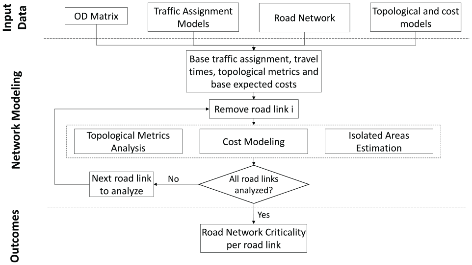
Road criticality framework.
The framework, as shown in Figure 1, presents a “full scan” process with
The network modeling starts with the base characterization of the traffic, topological metrics, and expected costs. These base measures represent the business-as-usual (BAU) patterns and costs. As the whole network is available, there are no isolated areas under this condition. Thereafter, the iterative process starts with removing each road link in turn to analyze how metrics change given the new road network configuration. Three different types of metrics are evaluated: (i) topological measures; (ii) expected increased costs; and (iii) isolated areas. The process continues analyzing one disruption at a time for the
A second analysis, focusing on multiple disruptions, was carried out using a Monte Carlo simulation. Figure 2 presents the framework for multiple road disruptions. This process aims to analyze how different metrics change as the network is increasingly disrupted. The process starts by defining a percentage of the network that is removed, followed by several realizations (different network disruption scenarios) per percentage. In each realization, road network disruptions were randomly sampled according to each percentage to estimate an expected value for each metric.
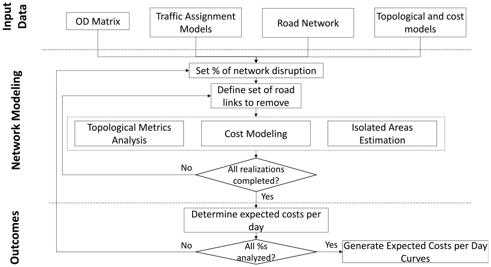
Multiple disruptions analysis.
After each disruption percentage is analyzed, the expected value of each metric is calculated according to Equation 1.

where
In this case, all realizations present the same probability of occurrence.
Both methodologies, single and multiple road disruptions, are designed to be adaptive and flexible in relation to the consequence models that can be incorporated. Therefore, although this methodology calculates the consequences in relation to topological metrics, expected costs, and isolated areas, other consequence models can be further incorporated, or indeed, other disruption costs can be added as further research becomes available.
Road Network Modeling
In this study, the road network modeling assigns traffic with the aim of quantifying expected travel times between each origin–destination pair, which subsequently allows the expected consequences of each road disruption realization to be calculated. The road network is represented by a graph
The graph construction involves the definition of: (i) road classifications; (ii) origin and destination points; (iii) road attributes; and (iv) spatial road network distribution. In this study, road classification refers to road hierarchy; origin and destination points define nodes in the network that generate or receive trips; road attributes are assigned to each link and include length, free flow speed, and flow capacity; and, finally, network geographical distribution defines the spatial relationship between different components. The Networkx library ( 43 ) was used to model the network.
The number of trips between each origin–destination pair can change after network disruptions. For instance, as a consequence of such realizations, users may decide to postpone or cancel their trips given a substantial increase in their travel time, or because of a complete disconnection of the network. In addition, the hourly variation of the traffic demand can be significantly affected by disruptions. Although the substitution problem has not been included in this study (when users change destination because of increases in travel times), a time threshold
Travel times are obtained following the user equilibrium principle, first proposed by Beckmann et al. ( 44 ). In this case, each user in the network aims to minimize their own travel time, and traffic flows are obtained by solving the optimization problem shown in Equation 2 subject to restrictions 3 to 6.

subject to


where
The constraint presented in Equation 3 establishes that the total vehicle flow must be equal to the demand for each particular pair
Several algorithms have been developed to solve this optimization problem, such as the Frank–Wolfe algorithm (
45
), method of successive averages (MSA) (
46
), or the incremental assignment algorithm (ITA) (
47
). The selection of a suitable algorithm depends on the network complexity, road agency goals, and traffic characteristics. This study considers a static incremental traffic assignment algorithm (ITA). This iterative process starts by defining a particular origin–destination pair
Topological Variables
Topological metrics focus on the spatial distribution and the structure of the network, while frequently neglecting dynamic features such as travel time or traffic flows ( 49 ). They are commonly related to graph theory. The topological metrics considered in this paper include betweenness centrality and closeness centrality.
Betweenness centrality is an important and frequently used topological metric that measures the importance of each element in the network based on their participation in minimum paths. This metric is defined as the ratio of the shortest paths passing through the link to all the shortest paths in the network (
11
,
50
). Equation 7 presents the betweenness centrality metric for any element

This metric has been widely applied to road networks to rank elements according to their topological importance ( 10 , 11 , 26 ). Furthermore, some modifications have been proposed in the literature to include other dimensions such as congestion ( 11 ), spatial heterogeneity of human activities ( 51 ), or travel times ( 14 ). This study considers road travel times as the main factor to compute shortest paths using the user equilibrium principle.
Another topological metric that is considered in this study is node closeness centrality, first proposed by Bavelas (
52
) in the context of social interactions. This metric measures the reciprocal of the average shortest path to node

Both betweenness and closeness centrality metrics are used to rank nodes and links according to paths that are shortest in travel times or traveled distances ( 53 ). Furthermore, Iyer et al. ( 54 ) related these metrics to network robustness, arguing that they reflect how a network can react to external threats.
Expected Impacts and Costs
Expected impacts and costs of disrupted road networks have been widely studied in transportation asset management ( 4 , 9 , 55 ). The main goal of these studies is quantifying different consequences of road network disruptions caused by external hazards. This study includes four consequence models: (i) vehicle operating costs (VOC); (ii) travel time costs; (iii) vehicle emissions; and (iv) number of isolated areas.
The VOC include fuel and oil consumption, tire deterioration, repairs and maintenance, and the proportion of deterioration related to vehicle use. Therefore, the estimation includes several variables such as vehicle class and type of road. The model adopted in this study corresponds to the one described in Waka Kotahi NZ Transport Agency ( 56 ) and is summarized in Equation 9.
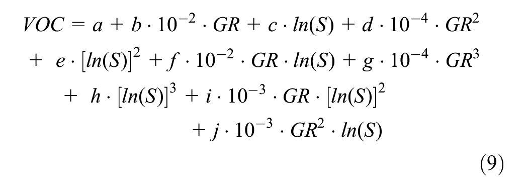
where
In addition, regression coefficients change according to vehicle class and road category (urban or rural roads).
Travel time value has been defined by several authors as the price people are willing to pay to have an additional unit of time ( 57 ), or the cost of marginal changes in time spent traveling ( 58 ). The total travel time value per hour can be calculated according to Equation 10 (adapted from Jayaram and Baker [ 59 ] and Cartes et al. [ 60 ]), where the total cost corresponds to the sum of all vehicle travel costs per road, for all roads.

where
The values were obtained from the methodology described in Denne et al. ( 61 ), which accounts for three different trip purposes (commuting, time-dependent, and flexible) and separate private and public transport.
Vehicle emission models include particulates


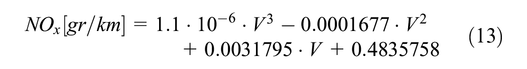

The valuations ($) of pollutant emissions reflect the damage caused to the surrounding environment, including to the ecosystem and people. Waka Kotahi NZ Transport Agency ( 56 ) estimated the monetary damage of each pollutant to the environment, and the respiratory/cardiovascular consequences to people based on the value of statistical life (VoSL). These studies are based on the previous work done by Kuschel et al. ( 63 ) and Austroads ( 64 ). Therefore, to calculate the total costs of each pollutant, the total emissions were multiplied by the costs per tonne obtained from Waka Kotahi NZ Transport Agency ( 56 ). Finally, the number of isolated traffic areas was calculated.
In this study, different types of nodes were defined to determine whether an area is isolated. As previously mentioned, nodes represent road junctions, origin and destination points, transportation hubs, and terminal points on the network. Areas of interest were assigned to different origin or destination points, and they were considered to be isolated when there was no access to more than two transportation hub nodes from that specific community node. In this case, transportation hubs were defined as airports, ports, and cities. Having access to ports or airport guarantees the exchange of good with external communities, and access to cities guarantees resources for a certain period of time.
Case Study Application: New Zealand’s South Island Road Network
This section applies the above methodology to an existing inter-urban road network in the South Island of New Zealand, and evaluates expected consequence changes in networks with different levels of redundancies, and how different disruption scenarios affect those consequences.
New Zealand is divided into two main islands; the North Island has a land area of 113,729 km2, produces 77.7% of the total national GDP and is home of 3,863,900 people; and the South Island has a land area of 150,437 km2, produces 22.3% of the total GDP and has a population of 1,178,900 ( 65 ). The geographical isolation of New Zealand, in addition to the high contribution of spatially distributed industries, such as forestry and agricultural, to the national economy highlight the strategic relevance of inter-urban road networks to maintaining domestic supplies, and guaranteeing access to the main ports/airports to retain international connectedness.
Although most of the national GDP is produced in the North Island (77.7%), the South Island is frequently affected by natural hazard events, such as the 2011 Christchurch earthquake, and 2016 Kaikoura earthquake. For example, the total GDP loss (in 2016 dollar value) caused by the Kaikoura earthquake was estimated at
New Zealand South Island Road Network Modeling
The network considered in this study corresponds to the New Zealand South Island inter-urban road network, encompassing the state highways, secondary, and tertiary roads according to the categories described in OpenStreetMap ( 67 ). This network has a total length of 11,814 km, of which 4,978 correspond to state highways and 6,836 correspond to secondary and tertiary roads, as shown in Figure 3. The state highways are managed by Waka Kotahi NZ Transport Agency, and the secondary and tertiary roads, hereafter referred to as “local roads,” are managed by the local authorities. To compare the two networks and analyze the effect of redundancy on road link criticality, the methodology is applied to (i) the state highways alone (red-colored in Figure 3) referred to as the “state highway network”; and (ii) the whole network (i.e., including state, secondary and tertiary roads) referred to as the “combined road network.” When converted into a graph, the state highway network alone includes 4,119 nodes and 4,204 links; whereas the combined road network has 12,982 nodes and 14,049 links.
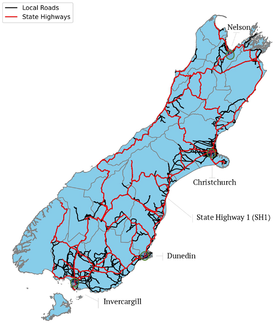
New Zealand road network (South Island).
The topographic information, as well as operating speeds and lengths for different roads, were obtained from OpenStreetMap ( 67 ), while the origin–destination and traffic data were obtained from Aghababaei et al. ( 5 ). This base model contains 541 traffic zones (TZs) based on NZ Census unit areas, and the supply and demand data were created based on three main travel purposes, namely commuting, tourism, and freight. Each traffic zone centroid was then linked to the closest node in the graph for further traffic assignment. Aghababaei et al. ( 5 ) obtained the data from New Zealand Census data, Regional Tourism Organization (RTO) website, and Ministry of Transport (MOT) data. According to this data, over 600,000 trips are completed per day in the case study area.
The road information from OpenStreetMap (
67
) was then converted into a graph using the
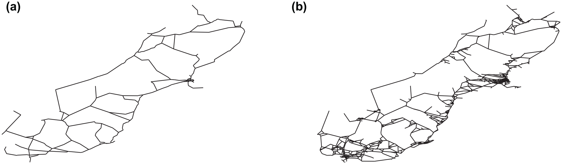
Road network graph representation: (a) state highway network and (b) combined road network.
The South Island road network modeling also includes the following considerations and assumptions:
The incremental traffic assignment algorithm (ITA) has been used in this study for its simplicity, convergence in simple networks, and fast computational time. In this study, road congestion is not considered and, therefore, travel times in each link do not change as a result of traffic assignment. While this can be considered a limitation of the model, traffic volumes for these inter-urban roads represent only a small portion of each road link’s capacity and, therefore, the inclusion of congestion models would not represent a significant change in the modeling outcomes. However, if traffic volumes are a considerable fraction of the road capacity, for example in urban case studies, congestion models should be incorporated. Furthermore, the presented assignment model (Equations 2 to 6) represents a general formulation and, therefore, includes a congestion model for completeness.
The traffic assignment model does not consider variations in the origin–destination matrix as a result of road disruptions. Therefore, users do not change destinations if their preferred route is blocked. However, the model does define a time threshold
The value of travel time, as well as the value of vehicle emissions and VOC, were obtained from Waka Kotahi NZ Transport Agency ( 56 ). For travel time, three different trip purposes have been considered: commuting, tourism, and freight. These three categories coincide with the categories in the origin–destination matrix.
Transportation hubs for the study area were defined as all the public airports in the South Island including Christchurch, Queenstown, Dunedin, Blenheim, Hokitika, Invercargill, Nelson, Takaka, and Timaru; ports include the ones located in Nelson, Picton, Lyttelton, Timary, Dunedin, and Bluff; while the cities as transportation hubs include Christchurch, Dunedin, Invercargill, and Nelson.
Multi road disruptions were carried out using Monte Carlo simulation. In this case, for each percentage of disrupted network, 500 iterations were analyzed to calculate expected values according to Equation 1. In each percentage, several disrupted roads are first defined. Subsequently, disrupted roads are randomly selected across the whole road network for each realization. Finally, metrics were estimated using Equations 7 to 14.
Road Network Criticality
Road network criticality is first analyzed for topological metrics, namely betweenness centrality and closeness centrality. Second, criticality is analyzed as the potential costs for users and non-users caused by each road’s disruption. In this sense, a road is more critical if it produces greater economic negative consequences when disrupted.
Figure 5 presents how the two networks present different topological values. In this case, when comparing the networks, the average betweenness centrality value for the combined road network compared with the state highway network decreases from, approximately, 0.094 to 0.025 (i.e., reduction of around 73%). This is directly related to the increased network redundancy and the available alternative routes. Lower betweenness centrality values imply that the network is less dependent on certain roads and disruption to them would produce less negative consequences. Although both networks result in the highest values occurring on State Highway 1, other roads in the combined road network present low values given the greater redundancy level of this network.
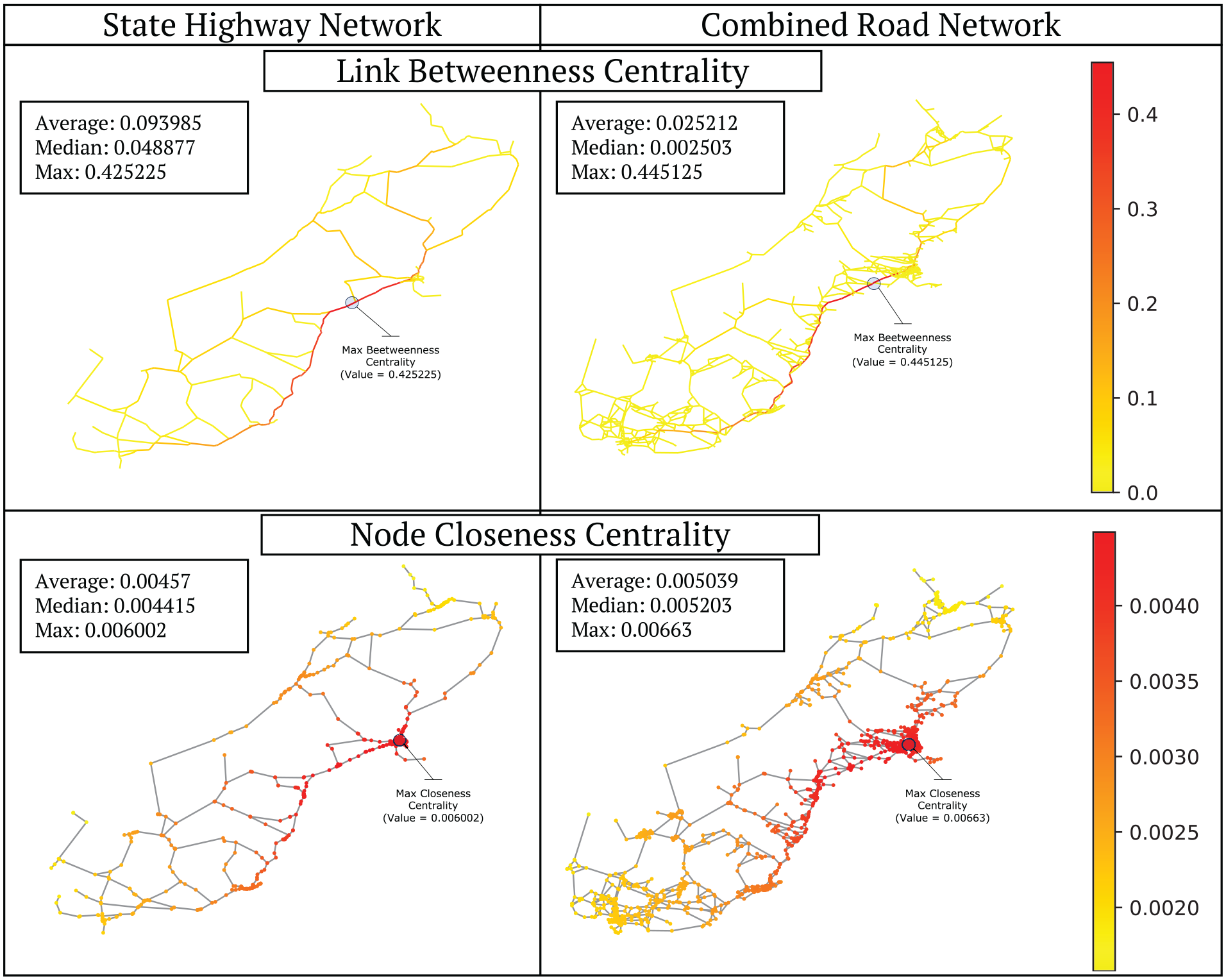
Topological metrics.
Average closeness centrality values increase in the combined road network. This means that nodes are, on average, closer to each other in travel times in the network with greater redundancy. However, the average value increases only 10.2%, which is significantly less than the 73% variation in the betweenness centrality average value. The closeness centrality value is highly dependent on the structure of the network and how the roads are located: as presented in Figure 3, most local roads are situated around the state highways and, therefore, the potential contribution of the local network to shorten the distance between all pair of nodes is limited.
Road criticality, that is, the economic consequences of road disruptions, is presented in Table 1. This table includes, for each metric presented in this document, the average and maximum increased cost of disruption of each road link disruption (i.e., the increased cost produced by each link disruption over the BAU expected cost). Those values correspond to daily consequences; it, therefore, considers the total number of trips per day. As presented in the methodology section, after each road was disrupted (removed from the network), a new equilibrium was then reached with the traffic assignment algorithm, and then the new metrics were estimated. Therefore, when a road is removed from the network, and the new equilibrium is reached, the increased overall cost was considered as that road’s criticality. Therefore, roads with greater expected consequence costs are considered as more critical.
Road Criticality (Increased Costs per Day)
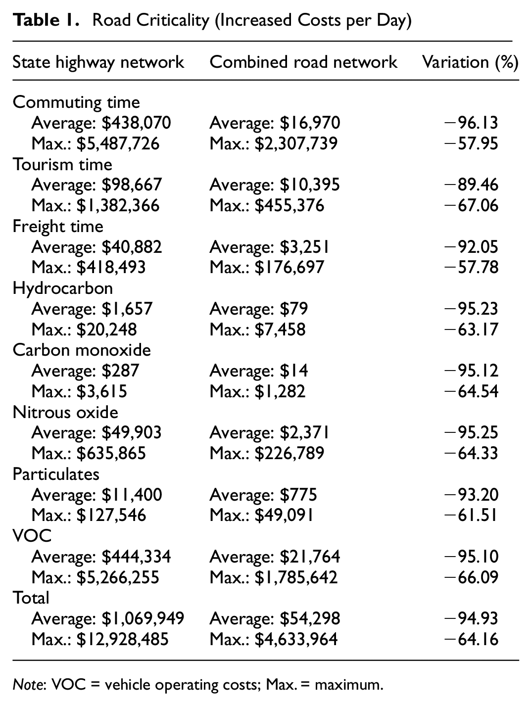
Note: VOC = vehicle operating costs; Max. = maximum.
In all the metrics presented in Table 1, the average and maximum values decrease with increasing redundancy in the network (from state highways only to the combined road network), demonstrating that secondary and tertiary roads contribute to reducing negative economic consequences caused by road disruptions. This is explained by the longer detours that users need to take when a critical road is removed from their paths, producing greater travel times, emissions, and VOC. However, although the decrease in maximum values ranges from 57.78% (freight travel time cost) to 67.06% (tourism travel time cost), the average values decrease significantly more, ranging from 89.46% (tourism travel time cost) to 96.13% (commuting travel time cost). Therefore, as expected, the state highway network is highly affected by the disruption of certain roads, while the impact of removing particular roads in the combined road network is considerably less. In addition, the significant reduction in the averages is mainly explained by the lower dependency of the combined road network on single road links. Furthermore, the number of canceled trips considerably reduces with increasing redundancy in the network. The average number of canceled trips reduces from 654 to 49 and the maximum number of trips canceled as a result of a single road link disruption decreases from 24,351 to 2,147.
Another aspect to be analyzed is the total number of canceled trips when disrupting each road. As presented in the methodology section, a trip is canceled when its travel time exceeds the time threshold
A graphical representation of daily total increased costs per road is presented in Figure 6, where the most critical links, and their total costs of disruption, are shown. This cost per link includes all the values presented in Table 1 integrated and, as shown in Figure 6, the most critical roads, in each network, are different. In the state highway network, the most critical roads provide access to Christchurch, while, as expected, they become less critical when the redundancy of the network increases. However, in both networks, the most critical roads are located in areas where the nodes connecting that road require a considerable detour to reconnect, and where the road is used by several vehicles. Therefore, as a direct consequence of this disruption, costly detours are added.
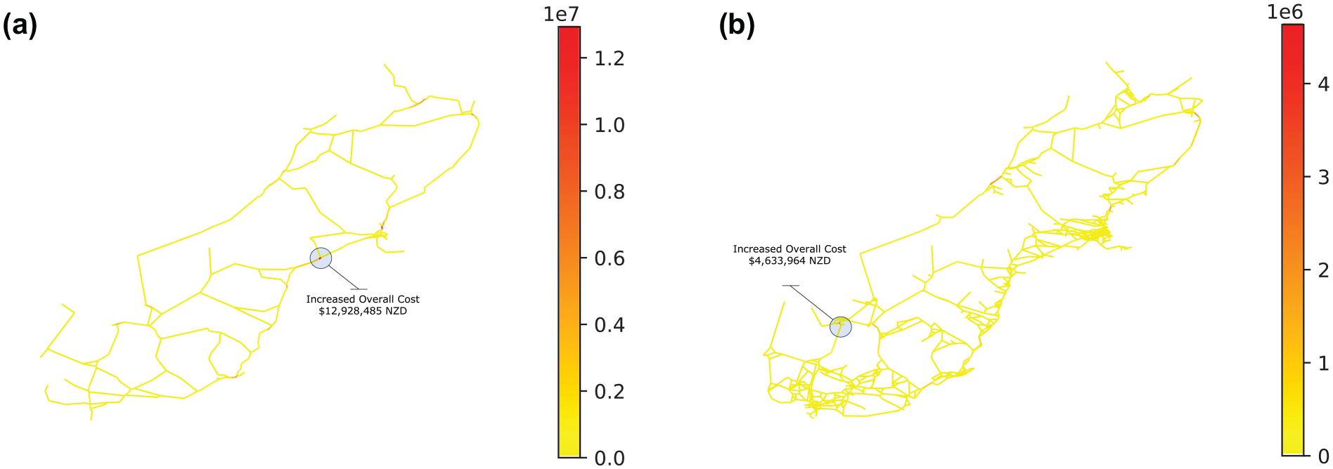
Daily total increased cost per road link disruption (NZD): (a) state highway network; and (b) combined road network.
To compare the two different criticality indices (i.e., betweenness centrality and the expected increased cost per road link disruption), we normalized all the values in a range from 0 to 1 using the min-max scaling method (
70
). Therefore, for both indices, the minimum value is set as 0, the maximum as 1, and any other value proportionally ranges within that interval, as shown in Figure 7. When comparing betweenness centrality normalized values to the total increased cost per link, the obtained
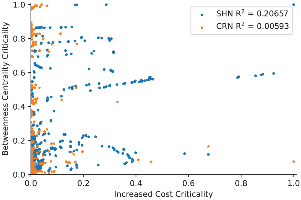
Criticality indices correlation.
The weak correlation observed when comparing criticalities is expected given that both measures have different underlying assumptions, goals, and mathematical approaches. While betweenness centrality evaluates the network’s criticality by measuring the number of times that each road belongs to a shortest path (for all pairs of nodes), the increased cost measure calculates the impact resulting from users’ disrupted travel patterns based on origin–destination matrices to define each link’s criticality. Despite these differences, and the obtained weak correlation, both methods are used in the literature to evaluate road network criticality. Consequently, decision makers should be fully cognisant of the differences between the metrics and adopt one that complements their own agency goals.
Multiple Road Disruptions
Multiple road disruptions were simulated by removing different percentages of the road network using Monte Carlo simulations as explained in the methodology section. Figure 8 presents how different costs change as the road network is increasingly disrupted and, therefore, trips are canceled. In this study, changes in users’ travel time costs, vehicle emissions, and VOC were considered.
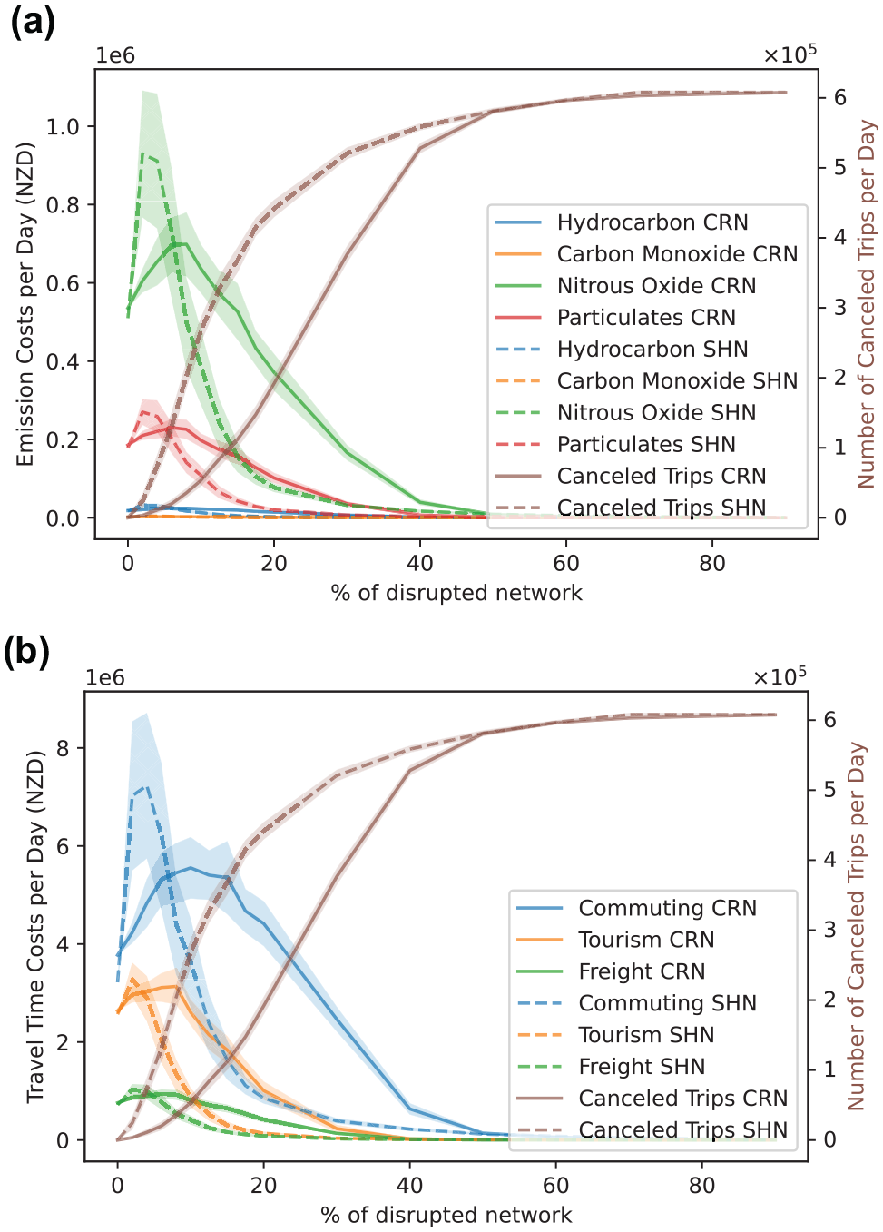
Consequences of disrupted networks: (a) vehicle emission costs of disrupted network; and (b) total travel time costs of disrupted network.
Figure 8, a and b , presents the vehicle emissions and travel time costs, respectively. In both cases, the results for the combined road network and state highway network are presented. In addition, the variability produced by the Monte Carlo realizations is also presented using the standard deviations for each curve. All curves show an increase of expected costs as the percentage of disrupted network increases, then reach a maximum value and, finally, they decrease. The decrease is explained by the number of trips canceled as a result of being in isolated areas (also presented in Figure 8). As a direct consequence of isolated areas and, therefore, canceled trips, an increasingly larger number of vehicles are not contributing to the total travel time, emission, and VOC costs.
The contribution of redundancy into reducing the effects of disrupted networks can be observed with two parameters: (i) maximum value; and (ii) curves’ increasing and decreasing rate. The first one identifies the maximum impact and associated percentage of disrupted network, while the second explains how robust the road network is, as explained by Iyer et al. ( 54 ). For instance, Figure 8a shows that the maximum nitrous oxide emission costs per day for the state highway network is $965,813 NZD and is reached with approximately 4% of the roads disrupted, while the maximum expected cost for the same pollutant on the combined road network is $715,169 NZD, which is reached with approximately 8% of the disrupted roads. After those two percentages, the expected costs decrease as the isolated areas and canceled trips increase. The curve’s increasing/decreasing rate is also a direct effect of the network redundancy. For example, as shown in Figure 8a, when 20% of roads are disrupted, the expected costs of particulates are $21,746 NZD (12.2% of the BAU scenario), and $102,438 NZD (55.2% of the BAU scenario) on the state highway network and the combined road network, respectively. As mentioned before, these values tend to decrease as the number of canceled trips increases (also shown in Figure 8). A slower decrease in costs, therefore, implies that road networks have viable detours, resulting in traffic reassignment.
Figure 8, a and b , also shows the number of canceled trips as the network disruptions increase. In this case, there is a direct correlation between the number of canceled trips and the decrease in expected costs (as those trips are not counted in the expected cost calculation). For instance, for the same 20% of disrupted network, the expected number of canceled trips for the combined road network and state highway network are 193,317 and 447,310 respectively, which corresponds to 31.79% and 73.57% of the total number of trips, respectively.
Similarly, expected travel time costs increase as the percentage of the disrupted network increases, then they reach a maximum value before decreasing. The maximum expected travel time cost values for the state highway network for commuting, tourism, and freight are $7,638,469 NZD, $3,218,902 NZD, and $1,026,961 NZD respectively, which are reached at 4%, 2%, and 4% of disrupted network. While the maximum expected travel time values in the combined road network are $5,536,558 NZD, $3,263,684 NZD, and $947,314 NZD, which are reached at 12.5%, 8%, and 8%, respectively.
The expected VOC are presented in Figure 9. In this case, the curves present the same trend as the expected travel time costs and emissions. The maximum expected VOC for the combined road network correspond to $6,424,528 NZD, and are reached when the disrupted network is around 8%, while the maximum expected VOC for the state highway network are $8,684,367 NZD and are reached when the disrupted network is around 4%. In this case, given the redundancy in the combined road network, the maximum expected VOC are reduced by 26%.
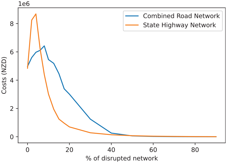
Expected vehicle operating costs (VOC).
Finally, the effect of different percentages of road network disruptions on isolated areas is shown in Figure 10. In this case, the expected isolated areas will increase as the percentage of disrupted roads increases. However, as explained for the other metrics, these two networks are affected differently because of viable alternative routes and network density. Although, eventually, both scenarios isolate 100% of the traffic areas (nodes), the isolation rate is different. For instance, the state highway network isolates 80% of the areas at 14.6% of disrupted roads, while the combined road network does it at 28.1% of disrupted roads. Furthermore, if we compare the percentage of isolated areas when 20% of roads have been removed from each network, the state highway network isolates 92%, while the combined road network only isolates 49% of the areas.
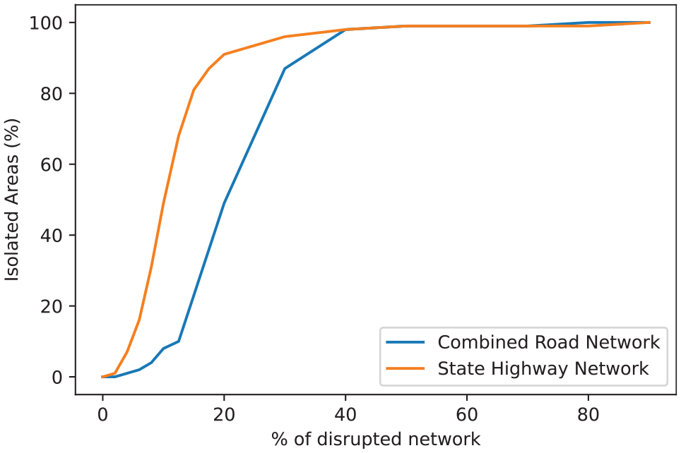
Isolated areas of disrupted network.
Conclusions
This research presents a methodology to estimate road link criticality through single-road disruptions, and expected overall consequences of multiple road disruptions. The single road analysis is carried out using the “full scan” method, and different metrics were evaluated after the new traffic equilibrium was reached. The multiple road disruption is evaluated using Monte Carlo simulation, generating different realizations using the same metrics. The methodology was applied to a road network in New Zealand’s South Island. In addition, topological metrics were evaluated to analyze road network criticality under different approaches. Finally, to evaluate the potential benefits of network redundancy, the secondary and tertiary inter-urban roads were added to the state highway network to create a combined road network for the analysis.
Increasing redundancy in road networks results in significant reductions in expected consequences and, therefore, criticality. For instance, the results of the single-road disruptions demonstrate that redundancy plays a key role when calculating expected costs and, therefore, road criticality. In particular, this study demonstrated how road network criticality significantly decreases as the network redundancy increases. For example, the disruption of the most critical link in the state highway network generates daily increased costs of $12,928,485 NZD, while the most critical link in the combined road network, which exhibits greater redundancy, generates a daily increased cost of $4,633,964 NZD, which is around 64% less. The same trend is observed in all single metrics, where the maximum value (i.e., the most critical road) decreases as the road network has more redundancy. This phenomenon is explained by the availability of shorter alternative routes in the network with greater in-built redundancy. As the redundancy increases in the network, users become less dependent on specific roads, given the opportunity of rerouting in cases of disruptions.
Similarly, redundancy is very relevant when evaluating multiple road disruptions. This approach was carried out using Monte Carlo simulation, where every realization was generated according to a specific percentage of the whole network. This approach is closer to how an external hazard (for instance, earthquakes, flooding, or even human-made events) may affect the road networks given their spatial distribution. However, this study considered uniform randomized disruptions, which are different to a specific hazard that tends to be more spatially localized. Results quantify the benefits of network redundancy in two different aspects: (i) redundant networks are less susceptible to experiencing significant increases in expected costs; and (ii) redundant networks generate more alternative routes to areas of interest, making them less susceptible to being isolated.
This study analyzes road link criticality based on topological attributes and potential economic consequences. When comparing these different metrics, differences were noted depending on whether or not the metric considers origin–destination information. On one side, topological metrics evaluate attributes based on the network structure and, although they consider roads’ travel time to calculate shortest paths, each node has exactly the same weighting. In this case, roads with shorter travel times are identified as the most critical, as observed in Figure 5, where State Highway 1 is considered the most critical road for minimum paths. On the other side, when considering origin–destination information, some nodes become more relevant than others given that they generate or attract trips, and all metrics evaluate their performance, directly or indirectly, according to travel times. These metrics mainly highlight roads that lack alternative routes, and are used by a lot of vehicles.
Furthermore, a comparison of criticality obtained by topological and economic analysis was undertaken by a correlation of resulting normalized values. This resulted in a weak correlation, demonstrating that the different methods lead to very different results and, therefore, investment decisions. In practice, each road agency determines which method they adopt, based on their stated priorities. In addition, other cost models could be added to the presented methodology, given its modular nature, and other dimensions such as access to critical infrastructure and potential costs of interrupted critical services (hospitals, schools, fire stations, etc.) could be considered when quantifying road link criticality.
The methodology in this study can be used by road agencies and decision makers to evaluate the effectiveness of different mitigation strategies, or post-disaster interventions, as it provides a tool to estimate expected costs of different road network configurations. Also, this study can be used to estimate the benefits of new road projects as it can estimate benefits of adding redundancy to the whole network. As demonstrated, network redundancy provides significant benefits in expected costs resulting from road disruptions, and the benefits of adding new roads showing in reducing those costs should be considered when evaluating a new project’s feasibility. Furthermore, this model can be used to define investment priorities when assigning resources. Given that the study identifies which road links produce higher increased costs when removed, a cost–benefit analysis could be considered by road agencies to prioritize their investment, where they could balance the mitigation investment costs against the potential saving of a more robust road link.
The study also revealed the need to extend the research to incorporate natural hazard modeling and infrastructure fragility curves. As explained, when evaluating multiple road disruptions in this study, roads were selected using a uniform probability distribution. However, in reality, the performance of road assets in response to a natural hazard event depends on the intensity and extent of the hazard, as well as the fragility of the assets. For example, earthquakes can affect vast areas, while riverine flooding or volcanic eruptions might affect limited locations. Furthermore, the magnitude of each event varies significantly, and the fragility of transport assets to each type of hazard could also modify the expected consequences. Therefore, such models should be considered when evaluating disruptions in road networks. Other research areas that could be incorporated include the estimation of the origin–destination matrix changes after a disruption to incorporate variations in demand, and the relationship between redundancy metrics at the network level and the expected increased operating costs. Furthermore, as demonstrated, as the road network is disrupted, trips may be canceled. However, the proposed methodology does not consider the economic costs of those canceled trips as an additional input for the road link criticality. Indeed, the cost of canceled trips might depend on several factors such as the type/duration of the natural hazard event (or any other disruption trigger), economic conditions of the study area, social vulnerability, and so forth. Consequently, the study also revealed the need to extend the research to include the development of a calibrated trip cancelation cost model to capture other potential benefits of resilience investments.
Footnotes
Author Contributions
The authors confirm contribution to the paper as follows: study conception and design: E. Allen, S.B. Costello, T.F.P. Henning; data collection: E. Allen, S.B. Costello, T.F.P. Henning; analysis and interpretation of results: E. Allen, S.B. Costello, T.F.P. Henning; draft manuscript preparation: E. Allen, S.B. Costello, T.F.P. Henning. All authors reviewed the results and approved the final version of the manuscript.
Declaration of Conflicting Interests
The author(s) declared no potential conflicts of interest with respect to the research, authorship, and/or publication of this article.
Funding
The author(s) disclosed receipt of the following financial support for the research, authorship, and/or publication of this article: The authors would like to thank the Resilience to Nature’s Challenges National Science Challenge, Grant project CO5X1901 for funding this research.