
Abstract
Fault identification is a recurrent topic in rotating machines field. The evaluation of fault parameters allows better maintenance of such expensive and, sometimes, large machines. Unbalance is one of the most common faults, and it is inherent to rotors functioning. Wear in journal bearings is another common fault, caused by several start/stop cycles – when at low rotating speed, there is still contact between shaft and bearing wall. Fault parameter identification generally uses deterministic model–based methods. However, these methods do not take into account the uncertainties inherently involved in the identification process. The stochastic approach by the Bayesian inference is, then, used to account the uncertainties of the fault parameters. The generalized polynomial chaos expansion is proposed to evaluate the inference, due to its faster performance regarding the Markov chain Monte Carlo methods. Deterministic and stochastic approaches were compared; all were based on experimental vibration measurements of the shaft inside the journal bearings. The Bayesian inference with the polynomial chaos showed reliable and promising results for identification of unbalance and bearing wear fault parameters.
Keywords
State of the art
Rotating machines are widely applied in power generation plants, oil and gas and transportation industries. Turbines, compressors and engines are the examples of these machines. Due to the widespread use of that kind of machinery, it is necessary to understand their nominal dynamical behaviour. With this purpose, mathematical models have been developed to reproduce the rotor’s dynamic response. Generally, shaft and disc models are solved by the finite element method, as proposed by Nelson and McVaugh 1 and Nelson. 2
Another crucial component of rotating machines is the journal bearing, which physical principle is mainly modelled by the Reynolds equation, see Reynolds, 3 based on the Navier–Stokes and continuity equations. Commonly, the solution of this equation leads to stiffness and damping coefficients that are added to the finite element model, as in Lund. 4 However, there are also nonlinear approaches, as given by Capone and colleagues5,6 and Machado et al., 7 where nonlinear forces represent these solutions.
The high cost of these machines makes maintenance procedures a mandatory issue. Consequently, to foresee possible faults through mathematical models is quite desirable. Besides, fault models enable fault parameter identification through the inverse problem concept. In this context, some faults as the residual unbalance level (according to the American Petroleum Institute – API standards) and the lubricated bearing wear, mainly caused by starts and stops of the system, are recurrent during the lifetime of these machines.
Aiming the identification of fault parameters, Markert et al. 8 developed a method that represents faults as virtual forces and moments, acting on the system. These virtual components were, then, inserted in the mathematical model of the healthy rotor. Thus, both conditions (healthy and faulty) can be compared, employing a least square fitting with the experimental data. Since the results were promising, this method is still one of the most used for fault identification. Similarly, Bachschmid et al. 9 treated the identification of multiple faults simultaneously, in which harmonic components of exciting forces and moments were used to model the faults.
Once unbalance is a frequent problem in rotating machines, the identification of unbalance parameters received special attention through the years. Sudhakar and Sekhar 10 used the method of the equivalent force minimization to search the unbalance parameters. Chatzisavvas and Dohnal 11 applied the least angle regression technique to obtain parameters of the unbalance. In this case, the main advantage of the proposed method is to avoid the necessity of previously known number of unbalances present in the rotating system. Later, Sanches and Pederiva 12 proposed an approach based on correlation analysis to obtain the parameters of shaft bow and unbalance simultaneously.
Despite unbalance, rotating machines supported by hydrodynamic bearings are also susceptible to bearing wear faults. Therefore, Papadopoulos et al. 13 developed a theoretical method to identify the radial clearance of worn bearings. Using a computational fluid dynamics (CFD) software, Gertzos et al. 14 calculated several bearing characteristics as a function of wear depth, applied to graphically identify the wear parameters. Machado and Cavalca 15 introduced directional coordinates to analyse the unbalance response and identify the wear parameters. Later, Mendes et al. 16 used directional frequency response function (dFRF), instead of unbalance response, to obtain the wear parameters, finding a good correlation with the expected values.
All model-based identification methods, however, assume deterministic approaches to the parameter estimation. The main point to be discussed here is about the accuracy and reliability of the whole identification process, which can be evaluated by probabilistic characteristics of the parameter itself, as well as the statistical distribution in the system response rebuilt.
Stochastic characteristics are presented in all kind of machines. When the information about a parameter is not completely known, a statistical approach should be applied in its modelling. Mechanical systems usually have stochastic attributes regarding design variables, due to manufacturing and assembly deviations, but also during operation condition, when the useful life determines the time degradation process, namely, critical fault conditions of the system. Therefore, in these cases, uncertainty quantification techniques are crucial to estimate variations in the system behaviour when subjected to random changes in physical parameters due to specific failures.
Recent research works applied uncertainty quantification techniques to analyse rotating machines.17–19 Monte Carlo simulations are an important approach to propagate uncertainties in the system response. However, the computational cost may be extremely high in some situations. An interesting option to avoid this problem is the application of generalized polynomial chaos, as proposed in the literature.17,18 However, limited prior information is a drawback for the latter approach in engineering problems. Another option is to apply a non-probabilistic approach, or mixed representation, for the uncertainties. 19 This research’s objective is to estimate fault parameters, when uncertainties should be considered, instead of dealing with uncertainty quantification. Thus, it is reasonable to assume for the priori distribution that the limits of the parameters are known (uniform distribution).
The Bayesian inference is a powerful tool to quantify fault parameters in rotating machinery, considering a stochastic approach. This method is based on the Bayes theorem and has made possible the update of the beliefs in random variables, called priori distribution. Marwala 20 used the method to update the parameters of a finite element model. Recently, Tyminski et al. 21 applied the Bayesian inference to identify journal bearing parameters of a rotating system. Mallapur and Platz 22 evaluated the best of four models to simulate the dynamical response of a real suspension structure.
The selection of the initial distribution to model the fault parameter (priori distribution) is crucial since it must correctly represent all the known information and the uncertainties of the related parameters. Jaynes23,24 presented the maximum entropy principle. This method uses the Shannon entropy to evaluate the distribution that considers all the uncertainty around the random variables. In the case of fault parameters, when the initial belief is a range of possible values, a uniform distribution is recommended as probability model.
A standard approach for solving the Bayesian inference, however, uses Monte Carlo via Markov chains (MCMCs), as seen in Beck and Au. 25 Although Monte Carlo methods are straightforward to implement and enable the use of deterministic solvers, they usually imply in high-computational cost, due to the huge number of samples needed for convergence. Therefore, for faster convergence, mitigating performance losses, the generalized polynomial chaos expansion (gPCE) can be used to approximate part of the Bayes theorem, as proposed by Nagel and Sudret. 26
Zhao et al. 27 applied the Bayesian inference with gPCE for prognostics of integrated gears, in which the observed crack propagation was used to update the remaining useful life of the gears. The authors compared the method with other procedures used for remaining useful life prediction, presenting good results. Garoli et al. 28 compared the identification of unbalance parameters in a Laval rotor through Bayesian inference solved by the MCMC and gPCE techniques. Both methods could identify the parameters correctly, although the gPCE solution presented a higher standard deviation. However, the gPCE needed 441 samples, while the MCMC used 10,000 samples.
Wiener 29 was the first author to present the gPCE, named ‘Homogeneous Chaos’, to approximate Gaussian processes through the Hermite polynomials. Ghanem and Spanos 30 used the polynomial expansion to develop a method able to evaluate the stochastic response of nonlinear random vibration problems. The method could evaluate stationary and non-stationary excitations as well. With the use of polynomial expansions, several statistical information of the solution, as the probability function, became more feasible.
Xiu and Karniadakis 31 expanded the Wiener’s idea of homogeneous chaos to non-Gaussian processes. Babuška et al. 32 proposed a method using polynomial expansion to solve random partial differential problems with Gaussian and exponential random variables. The authors presented an extensive convergence analysis and strategies to use the collocation method for evaluating the expansion coefficients. Ni et al. 33 described the advantages of the gPCE method over the Monte Carlo simulations through the stochastic response evaluation of a bridge structure. Sinou and Jacquelin 34 calculated the stochastic steady-state response of an asymmetric rotor using polynomial expansion and comparing it with the Monte Carlo method. The polynomial expansion presented good results, but the response was sensitive to low-level polynomials. A recursive method was developed, and a convergence criterion was defined.
Summarizing, model-based identification of fault parameters in rotating machines is commonly a deterministic approach, although the experimental data always present several sources of uncertainties. In this way, to obtain a reliable solution, a stochastic approach should be used. The present work proposes the application of Bayesian inference to identify the parameters of two different faults (unbalance or bearing wear) in a rotating machine. Consequently, to avoid unnecessary time-consuming, the polynomial chaos expansion is applied. The results obtained by the stochastic method are compared with those obtained by the deterministic identification, showing the strength of the proposed approach.
System modelling
Rotor modelling
In the rotordynamics field, the finite element method has been traditionally used to represent continuous rotating systems, since it permits the coupling between translational and rotational motion. 35 A schematic rotating system and its reference system are presented in Figure 1.
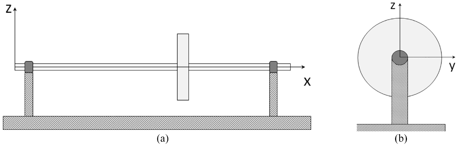
Rotor system scheme.
Using the Timoshenko beam element 1 for modelling the shaft, in which each node has 4 degrees of freedom, two translational and two rotational, and the rigid disc model for the discs, it is possible to find the equation of motion of the rotating system applying the Lagrange formulation. Thus, the complete equation of motion is written as 36

where
Bearings must be considered in the system model as well. If the journal bearings operate under the hydrodynamic regime (Figure 2), the sustaining forces can be evaluated by the pressure distribution given by the solution of the Reynolds equation. This equation can be obtained from momentum and mass conservation for a Newtonian viscous fluid, under appropriate hypotheses. Equation (2) gives the Reynolds equation 3
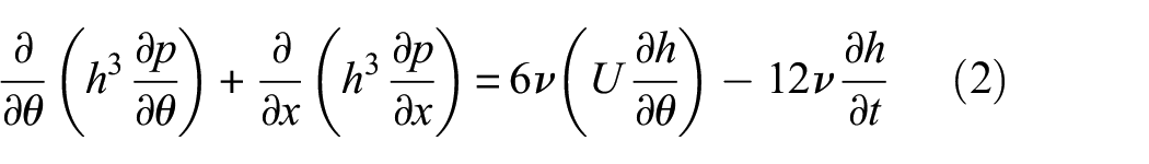
where θ and x are the circumferential and axial coordinates, respectively, p is the pressure distribution, U is the tangential velocity of the shaft, ν is the oil film viscosity, and
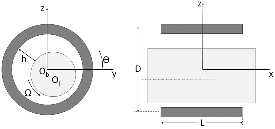
Bearing system.
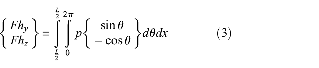
The complete solution of the Reynolds equation, which gives the pressure distribution inside the bearing, can only be achieved by numerical procedures. For this purpose, the finite volume method was employed. The pressure field must be integrated to evaluate the hydrodynamic forces
Usually, bearings are represented by stiffness and damping coefficients, which are obtained through linearization of the hydrodynamic forces around the journal equilibrium position inside the bearing, giving a good approach for a wide range of operation (for more details, see Machado et al. 7 ). Then, according to Lund, 4 the hydrodynamic forces can be rewritten as
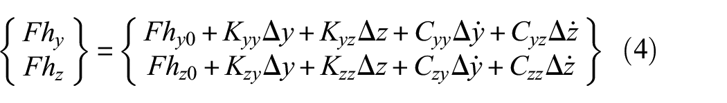
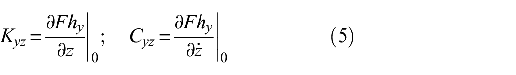
and the coefficients are the partial derivatives of the forces evaluated at the equilibrium position 38
The dynamic coefficients are summed in the shaft’s stiffness
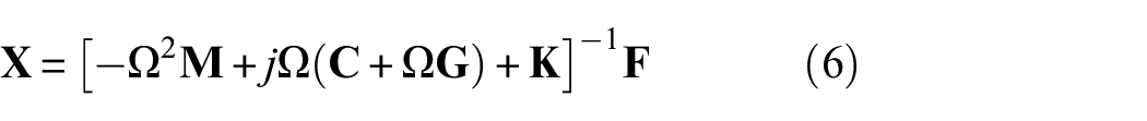
Equation (6) gives the solution of the equation of motion in the frequency domain. However, if the solution needs to be in the time domain, the equation of motion has to be numerically integrated. For this purpose, the Newmark integrator was employed. 39
Unbalance modelling
Certainly, mass unbalance is not a new or even a complex fault. However, it is the most common source of vibration in a rotating machine, and it will be the first fault analysed in this article.
The unbalance force comes from the resulting inertial force caused by an amount of mass displaced from the centre of rotation. As well known, it can be vectorially written as
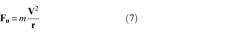
where m is the unbalanced mass,
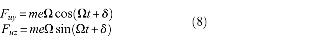
where e is the magnitude of vector
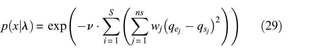
As previously said, for fault identification, experimental and theoretical vibration signals should be related through an objective function. For the unbalance identification, since the machine will operate in a pre-determined and fixed rotation, the most common vibration signal is the spectrum, or the discrete Fourier transform (DFT), of the journal displacement inside the bearings. For this reason, the objective function used was the least square formulation shown in equation (9)
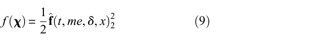
where
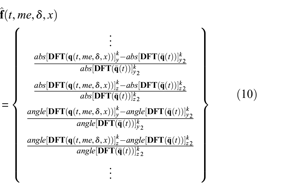
where
Wear modelling
Besides the unbalance, bearing wear is also prone to occur in rotor systems supported by hydrodynamic bearings. The wear model used here was presented by Machado and Cavalca,
40
in which the authors expanded the abrasive wear model initially proposed by Dufrane.
41
Consequently, the wear parameters become the maximum wear depth
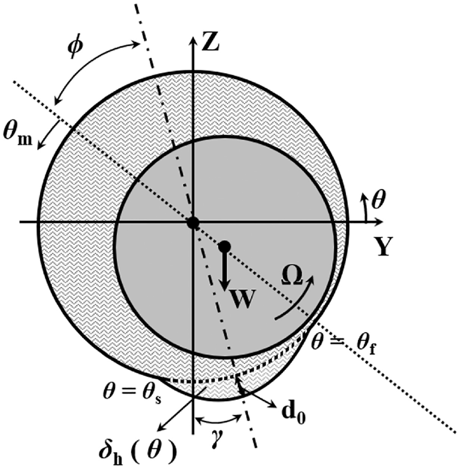
Worn bearing.
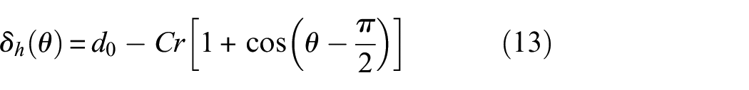
The wear introduces additional thickness to the oil film, so the expression for the new oil film thickness becomes

The original oil film thickness
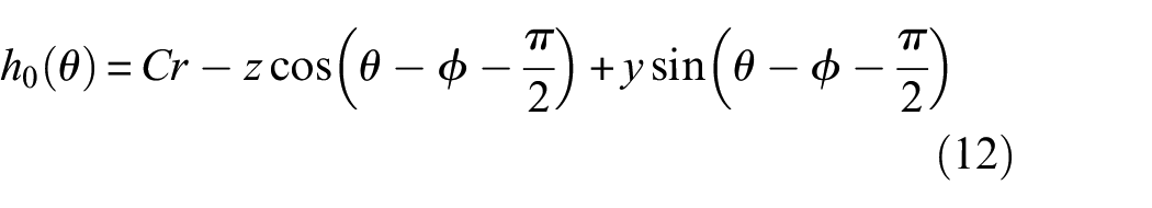
where ϕ is the attitude angle.
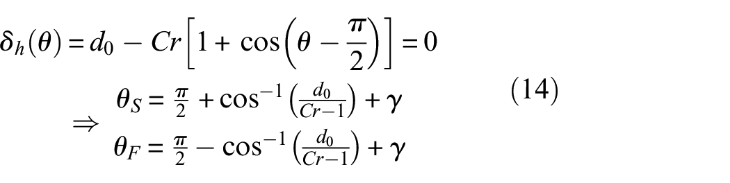
For the angular boundaries of the wear, the additional thickness is null. Thus, it is possible to precisely obtain the extreme points of the wear region. Therefore,
Finally, the oil film thickness is given by
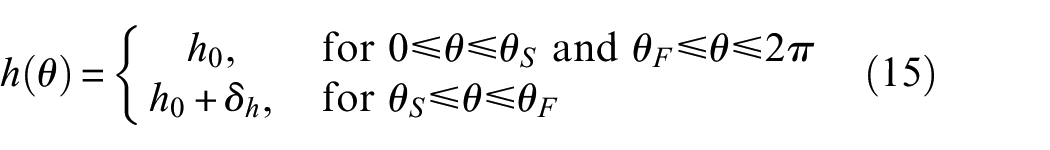
Then, the new oil film thickness in equation (15) substitutes the previous one in the solution of the Reynolds equation. At this point, it is necessary to compare the experimental vibration with the numerical simulation results. Thus, the least square function is used on a logarithmic scale, according to equation (16)
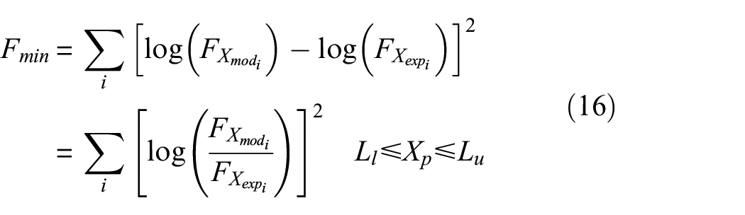
where
It is important to say that, in equation (16), the frequency responses of the rotor-bearing system, both experimental and numerical, are used in directional coordinates because of its sensitivity to the influence of anisotropy, which tends to increase the backward component in the presence of wear (Machado and Cavalca 15 ). Note that the least squares method was used in both objective functions because it is a traditional and simple technique, while highly robust. As it satisfactorily performed the adjustment, there was no need to test other methods for the purpose of this work. Detailed and actual discussion about efficient approaches to solve least squares problems can be seen in Birgin et al. 42
The objective function considered for unbalance identification, shown in equations (9) and (10), considers the DFT of a time-domain signal. This equation is specifically related to the unbalance case, since dealing with absolute differences between harmonics in the DFT spectrum.
However, the objective function in equation (16) is related to wear identification. Here, the unbalance response is considered in the frequency domain. In this case, the convergence of the search method tends to be difficult when working with simple least square as the objective function, especially due to a large number of abrupt variations and, therefore, local minima. It is also important to highlight that since we are dealing with frequency response, there is a great variation in the response amplitude. To overcome this problem, Arruda 43 proposed the use of a logarithmic scale for modelling the objective function, which tends to improve convergence in the searching process. The logarithmic function aims to weight the values of the objective function in the frequency range, that is, there are no sudden changes near the resonance region.
Deterministic identification
For model-based identification, in order to relate fault with its effects on the system, a reliable model of this system must be developed. Then, the information obtained through the numerical model (theoretical data) must be compared with the measured vibration data (experimental), and a minimization of the residual difference must be accomplished. This procedure leads to the fault parameter identification.
Independently of the minimization technique employed, being it stochastic or deterministic, it is necessary to determine the objective function and the information to be processed in it. Therefore, the objective function should express the essential elements of the problem, and among several possibilities, the least square method is widely used for comparing two sets of data. As presented in section ‘System modelling’, equations (10) and (16) are defined to be used in the unbalance and bearing wear cases, respectively. In addition, for rotating machines, the most used information is the vibration signals, usually measured at the bearing positions.
Being the numerical model of rotors obtained by the finite element method, the fault parameters associated with the position along the length of the shaft must have only discrete or integer values. This fact adds extra difficulty in the optimization problem since it becomes a mixed-integer nonlinear programming (MINLP).
Solution for the MINLP
An MINLP can be mathematically described by equation (17)
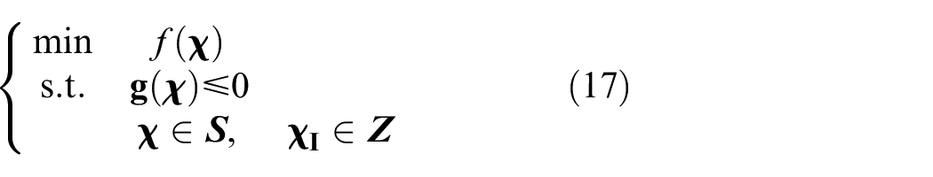
where
According to Bonami et al.,
44
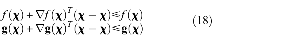
several techniques have been developed to solve MINLPs in the last decades, among them, the outer approximation. This specific technique proposes that an MINLP can be represented by a mixed-integer linear programming (MILP) through linearization of the objective and constraint functions around a given point
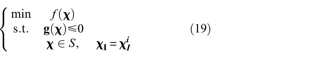
The point, which the functions can be linearized around, is determined by solving a subproblem generated from the original MINLP. For this, all integer variables are fixed in pre-determined values
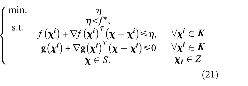
In addition, an MINLP can have its objective function further linearized replacing the original objective function by an auxiliary variable η. This new variable should have a value lower or equal to the previous nonlinear objective function. Then, defining
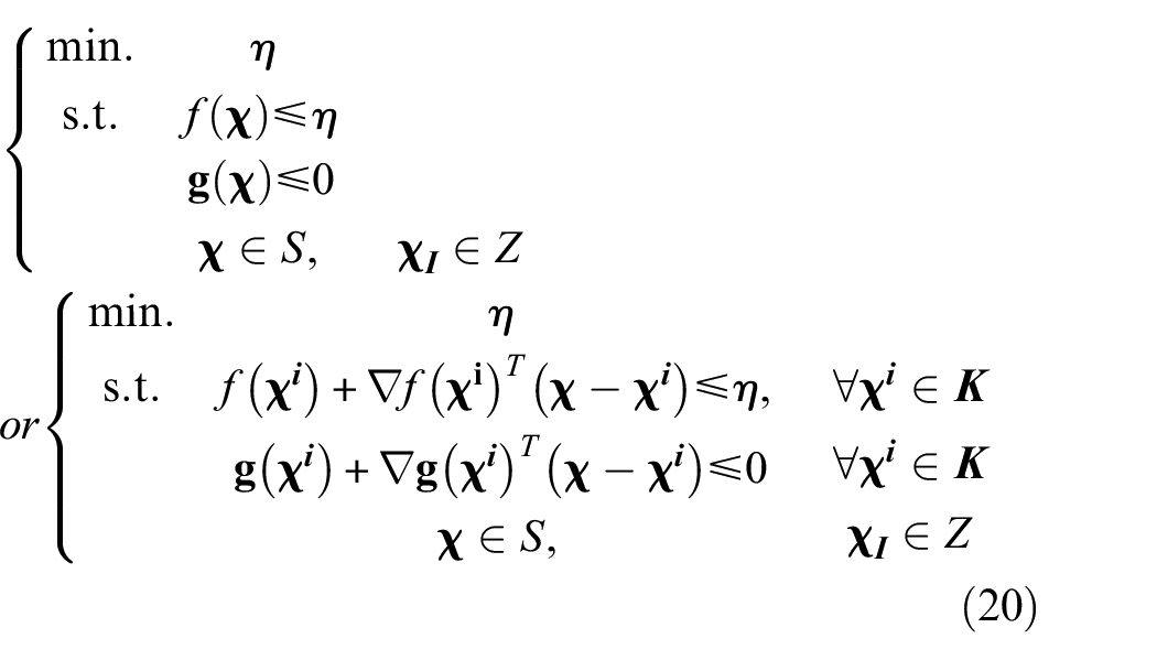
Therefore, the outer approximation method proposes to solve MILPs and fixed NLPs alternately. First, an NLP subproblem fixed at an initial condition
Since new points are successively inserted into set
Solution for the NLP
Usually, the variables in an identification problem are subjected to value constraints, making the NLP a constrained optimization. However, it is possible to approximate a constrained optimization into an unconstrained optimization using the barrier method (Bazaraa 45 ). The barrier method introduces an additional term to the objective function that prevents the variables from having unfeasible values, that is, violating the constraints. Then, a sequence of feasible points is created. So, the barrier problem is defined as
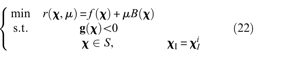
where μ is the penalization parameter, and
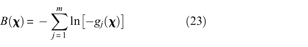
where m is the number of constraints.
Thus, a decreasing sequence for μ is created, and equation (22) is solved by any unconstrained optimization method for each value of μ, until
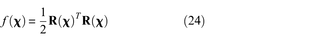
where
To solve this optimization problem, the method proposed by Dennis et al., 47 which is based on the quasi-Newton scheme, is used. Therefore, the descent direction can be calculated by equation (25)
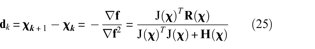
where
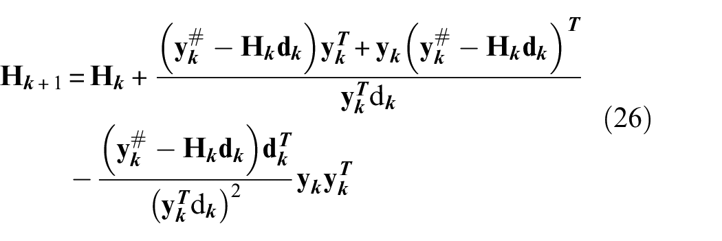
and
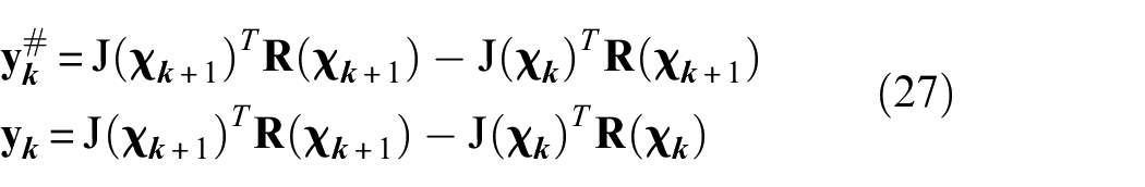
To improve the effectiveness of the descent direction, it is possible to calculate step length that improves the objective function value, that is,
Solution for the MILP
One of the most common techniques to solve mixed-integer optimization problems is the branch and bound method (Morrison et al.) 51 For this reason, it will be used in this article for solving the problem shown in equation (21). To find the optimal point, the method builds a tree containing subproblems that are subspaces of the set S. Moreover, it stores the best feasible solution – known as the incumbent solution. Hence, for each iteration, the algorithm explores a new subspace finding a solution for it. If the new solution is feasible, integer, and has an objective function value smaller than the stored one, the incumbent solution is updated. However, if the feasible solution has higher objective function than the stored one, the subproblem is cut from the tree. If there is no integer solution, the subproblem is split into two new subproblems, which becomes new branches of the tree. When all subproblems are explored, the best incumbent solution is returned.
Therefore, the MILP from equation (21) is relaxed for the integer variables, becoming a simple linear programming (LP) optimization that can be solved by the simplex algorithm (Luenberg and Ye 46 ). An optimal point is found when the solution is feasible and integer. Otherwise, one uses the branch and bound technique to find a new MILP.
Bayesian inference
Specific procedures to the stochastic identification enable to take into account the stochastic aspects of the fault parameters identification, namely, the statistical distribution associated with each fault parameter and, consequently, their confidence bounds.
To identify the unbalance and bearing wear parameters, the Bayesian inference was implemented together with the gPCE. This statistical inference uses the Bayes theorem to update the distribution of a random variable of interest given evidence or observation.
Bayes theorem
The theorem, named after Thomas Bayes, uses the conditional probability to update the beliefs of an event. Bayes was the first to present the idea of conditional probability, which measures the probability of an event
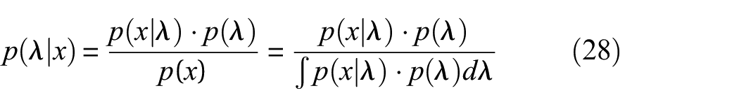
In equation (28),
where
where
gPCE
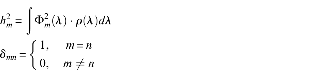
For evaluating the posteriori distribution faster than MCMC methods, it was implemented the approximation of the likelihood distribution through gPCE. Equation (31) shows the truncated polynomial series, which has a maximum degree P
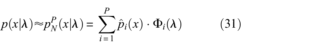
In equation (31),
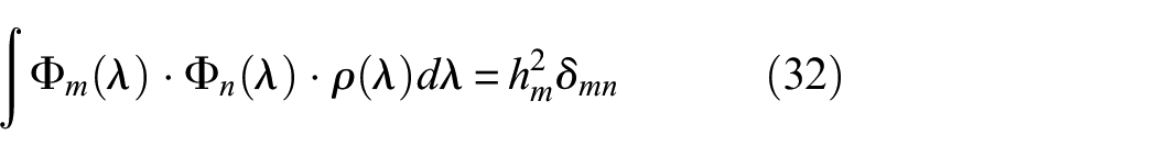
where
Polynomial families are related to random variables through the weighting function
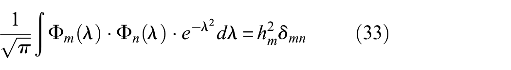
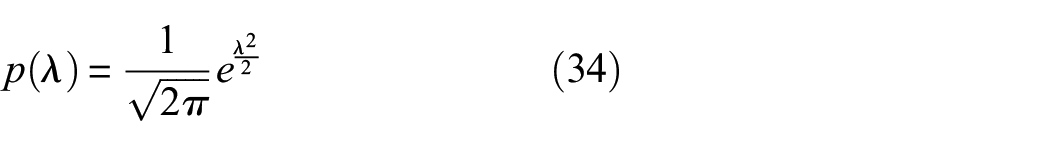
For problems with
with
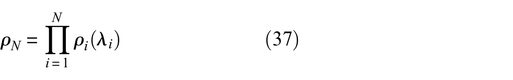
And the joint PDF of the polynomial basis is given by
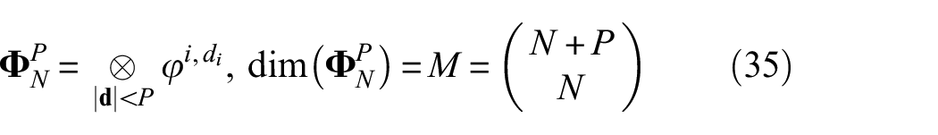
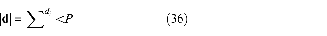
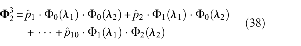
For a better understanding, an example of a polynomial basis for
From equation (35), it is known that the dimension of the polynomial basis is
Using the gPCE approximation, the problem to be solved is the identification of the expansion coefficients.
Stochastic collocation
For evaluating the expansion coefficients, the stochastic collocation was used. The method consists in evaluating samples on pre-chosen nodes and, then, solving the system presented in equation (39)
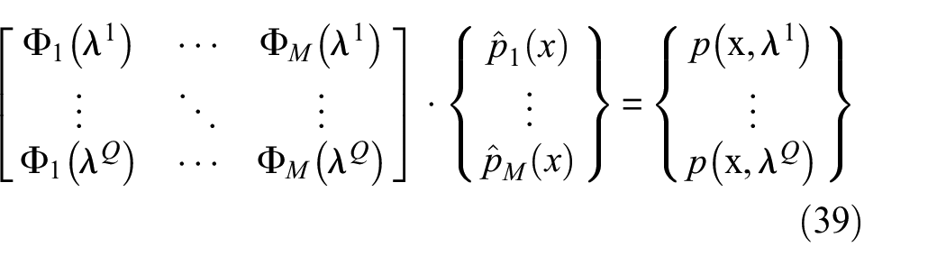
where
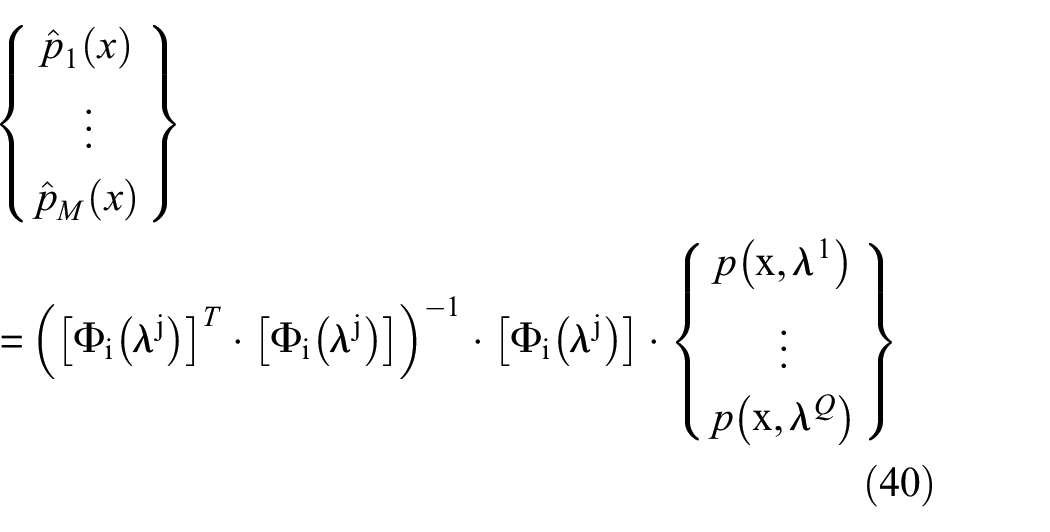
In this work, the nodes are equally spaced between the limits of the variables to be identified. For a better approximation, the linear system becomes overdetermined. Therefore, the least square method is used, as presented in equation (40)
The convergence of the gPCE can be evaluated by sparing some samples, calculating the difference between these spared samples and the gPCE results. This procedure can help with the analysis of the convergence and avoid over-tuning the approximation.
Solving the Bayesian inference
Commonly, MCMC methods are utilized to evaluate the posteriori distribution by constructing a chain of samples that respects this distribution. However, as said before, these methods need a considerable number of samples and, if it is a time-consuming simulation, the time needed to evaluate the posteriori distribution may become unfeasible.
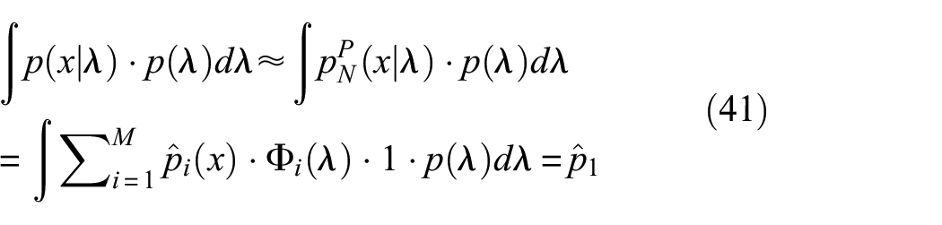
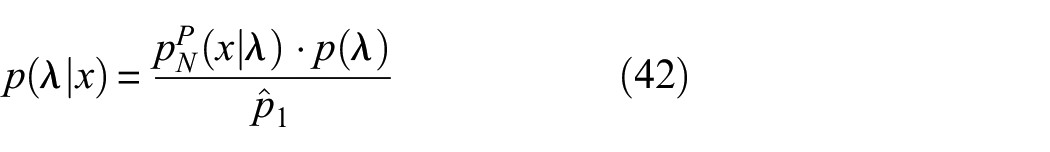
The polynomial approximation facilitates the solution of the integral term in the Bayes theorem, due to the orthogonality propriety of the basis, see equation (39). Finally, the posteriori function is the product between a known distribution and a polynomial series, as shown in equation (41)
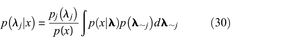
The posteriori marginal distribution, which is the posteriori distribution of just one parameter, is evaluated by equation (43)
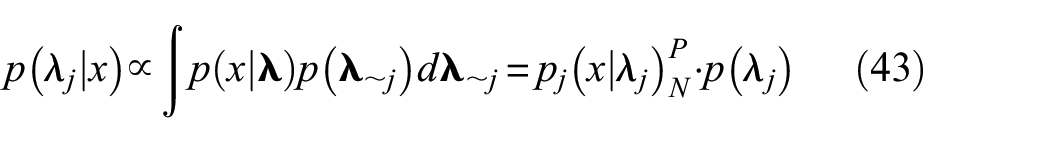
Putting into words, the marginal posteriori functions are all the terms of the full polynomial series that are only dependent on
Experimental test rigs
The application of both deterministic and stochastic methodologies, described in sections ‘Deterministic identification’ and ‘Bayesian inference’, involves two different assemblies of the test rig, aiming initially to observe each model performance with the specific fault parameters to be identified. Therefore, for the unbalance parameters identification, a long and slender shaft was assembled to highlight the precession (whirl) effect related to this fault. However, for wear the parameter identification, a shorter shaft is used to stress the bearing effects, helping to mitigate excessive unbalance effects.
The identification of the presented faults was made using different types of vibration responses from the rotating system. The unbalance fault is well characterized in the frequency spectrum of the signal, being its signature the 1× component of the DFT, if considered a predominantly linear system. Therefore, the time response obtained directly at a specific operating rotation speed was used. This type of response is the easiest and most directly obtained in real systems, adding a practical character to the application of this article.
However, as the wear signature in the frequency spectrum of the response is not yet fully established, the unbalance response in the frequency domain was adopted. In addition, as it is known that this type of wear increases the system anisotropy, the use of directional coordinates more clearly shows the effects of wear variation.
Unbalance experimental test rig
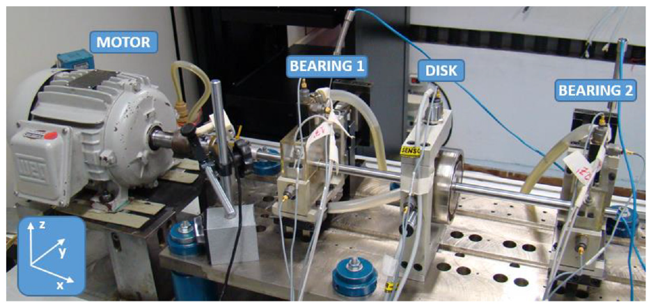
The test rig designed for unbalance parameter identification purposes is represented in Figure 4. In this configuration, the shaft – 603 mm long and 12 mm in diameter – is supported by two identical hydrodynamic bearings (nodes 4 and 15 in Figure 5). The bearings are 31 mm in diameter, 18 mm wide, with 90 µm of radial clearance and viscosity of 65 mPa s. The first bearing is approximately located at 124 mm from the flexible coupling (node 1 in Figure 5), while the second bearing is located 400 mm from the first bearing. There is also a journal (nodes 6 to 8) located at 37 mm from bearing 1 and a disc, 47 mm long and 94.7 mm in diameter, at 65 mm from bearing 2. The 3.2-g unbalance mass inserted in the system is located on the left side of the disc – node 10 of the finite element model in Figure 5– with a radial eccentricity of 37 mm from the centre of the disc. The actual unbalance is 1.184 × 10⁻⁴ kg m at a phase angle of 300° (−1.054 rad) relative to the horizontal reference axis. The rotating speed for the test is 49.3 Hz, which is the first critical speed of the rotor in this configuration.
Experimental test rig for unbalance.
Finite element model for the system in Figure 4.
Rotor-bearing systems supported by cylindrical journal bearings present fluid-induced instability. Hence, the rotating speed for the unbalance test is below the threshold of instability since it is close to the rotor first critical speed.
Displacement signals are measured at the bearings positions at a sampling rate of 4096 samples/s for a total test time of 2 s. In addition, the signal is collected five times to exclude possible random errors.
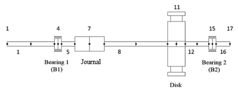
The finite element model for this test rig configuration is shown in Figure 5 and consists of 16 Timoshenko beam elements and three rigid discs elements, overlapped at node 11. The discs presented in both experimental assemblies are modelled using rigid disc elements, which have only inertia and gyroscopic effects concentrated in a single node, as presented in Nelson and McVaugh 1 and Nelson. 2 The thickness is used just for calculating the disc’s moment of inertia in each direction. To represent the geometry of the real disc, which has a recess for including small unbalance masses, three disc elements were used with different diameters, being one of them with a smaller thickness to represent the recess. Also, in the beam elements used to model the shaft portion along the disc length, the diameters are slightly increased to take into account the stiffening effect due to the rigid disc thickness, according to Lalanne and Ferraris. 36
Bearing wear experimental test rig
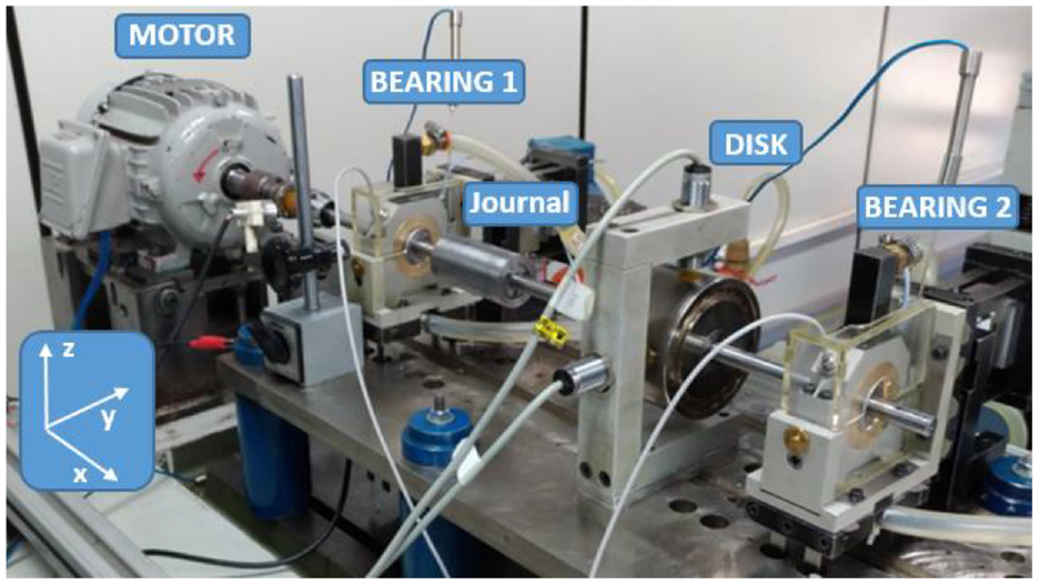
In this case, a Laval rotor is assembled as in Figure 6. The shaft, 478 mm long and 12 mm in diameter, is supported by two identical (except for wear on bearing 2) hydrodynamic bearings (nodes 4 and 14 in Figure 7). The bearings are 31 mm in diameter, 18 mm wide, with 90 µm of radial clearance and viscosity of 65 mPa s. The first bearing is approximately located at 97 mm from the flexible coupling (node 1 in Figure 7), while the second bearing is located 400 mm from the first bearing. There is also a disc, 47 mm long and 94.7 mm in diameter, at 152 mm from both bearings. The 1.7-g unbalance mass is located on the left side of the disc, node 9 of the finite element model in Figure 7, with a radial eccentricity of 37 mm from the centre of the disc. The wear is placed only in bearing 2 (B2). The actual wear parameters are depth (d0) of 20.52 µm and angular position of wear (γ) at 21° from the vertical axis in counter-clockwise direction.
Experimental test rig for bearing wear.
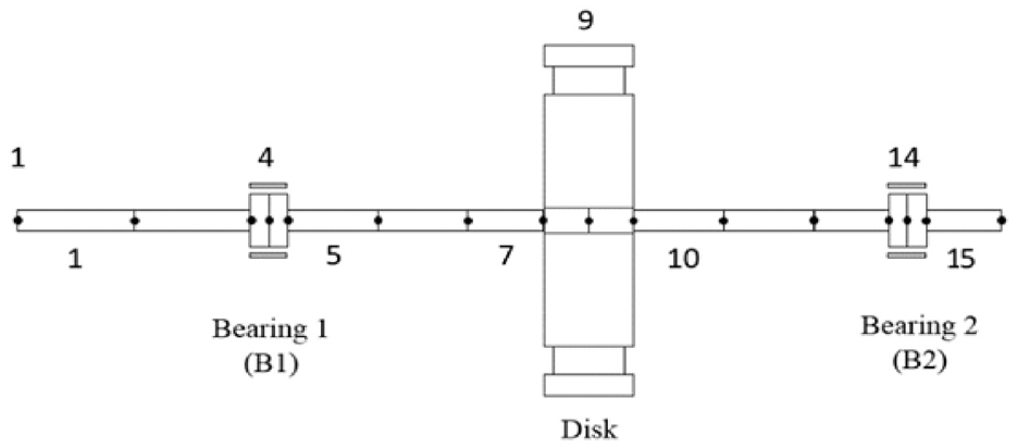
Finite element model for the system in Figure 6.
Displacement signal measurements are repeated 10 times to obtain the orbit amplitude average at the worn bearing. For each rotating speed, in the range from 10 to 74 Hz with a step of 0.5 Hz, the orbital position is acquired at a sampling frequency of 2048 Hz during a test time of 8 s. Again, the rotating speed range is below the instability threshold.
The unbalance response function is then obtained, and it can be represented in directional coordinates, namely, forward and backward components. In addition, the finite element model for this case is shown in Figure 7 and consists of 15 Timoshenko beam elements and three rigid disc elements (similarly to Figure 5), overlapped at node 9.
Parameter identification results: stochastic and deterministic
The theories related to deterministic and stochastic parameter identification, respectively, presented in sections ‘Deterministic identification’ and ‘Bayesian inference’, are, therefore, applied to the experimental data and compared with the rotor model subjected to unbalance and bearing wear faults.
Unbalance identification
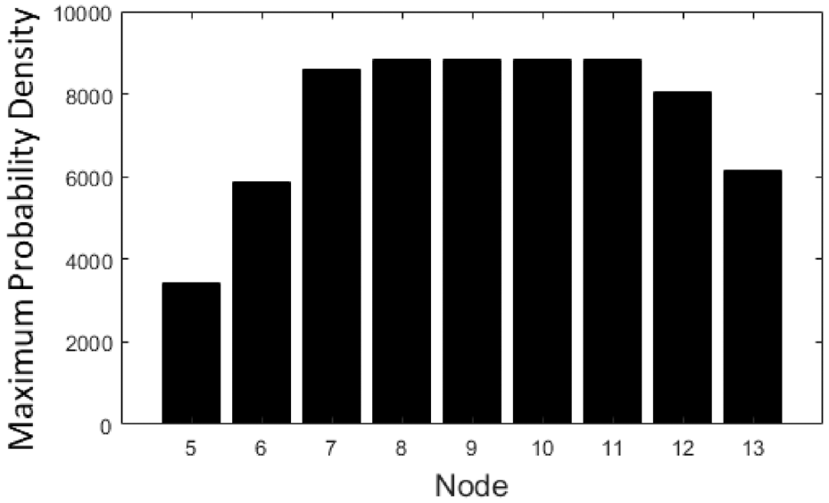
The first set of results concerns the unbalance identification. As previously stated, an unbalance of 1.184 × 10⁻⁴ kg m in a phase of −1.054 rad was placed on the left face of the disc. As for the deterministic case, the stochastic approach also suffers from the additional difficulty imposed by a discrete variable for the unbalance axial position. So, to avoid manipulating a discrete variable, the identification was run for each node separately, and Figure 8 shows the maximum probability density of the unbalance moment at all nodes between the bearings.
Maximum probability density at the nodes between the bearings.
The priori distributions of both parameters are modelled by uniform distributions. The unbalance value is between 10−5 and 10−3 kg m and the unbalance phase value is between −π and π rad. For each node, the Legendre polynomials with a maximum degree of 8 are considered, resulting in a basis of 23 terms, with a grid of 400 points.
Observing Figure 8, nodes 8–11 have a higher maximum probability density. It is interesting to note that these nodes are the central ones (in between the bearings), and an unbalance force at these nodes will easily excite the first bending mode, which is the operational mode of the rotor. Taking a closer look at Table 1, which shows the values of maximum probability density at nodes 8–11, one can see that the maximum probability density for node 8 is slightly lower. So, for further analysis, this node can be discarded. Moreover, node 9 lies far from the disc position, where the unbalance masses can be inserted, and for this reason, it can also be discarded.
Values of the maximum probability of nodes 8–11.
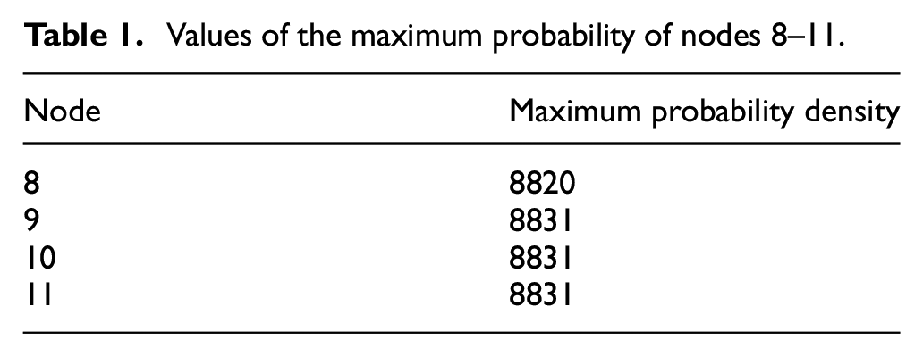
Therefore, according to the Bayesian inference, nodes 10 and 11 have the same probability density of hosting the unbalance mass, being the real unbalance located at node 10. If no information about the node is previously known, as it happens in most practical situations, and if more than one node has the same probability density of holding the unbalance mass, a comparison between the experimental data and simulation, with the parameters given by the identification (for the indicated nodes), must be accomplished. A way to do such kind of analysis is observing the objective function value, presented in Table 2, pointing to node 10 as the best solution for the unbalance axial position.
Objective function values.
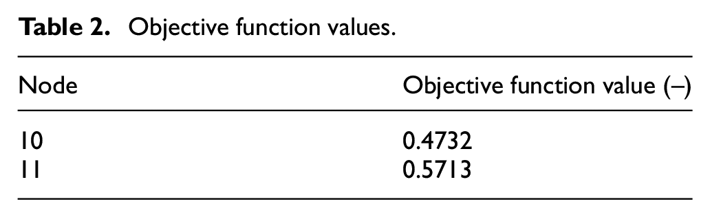
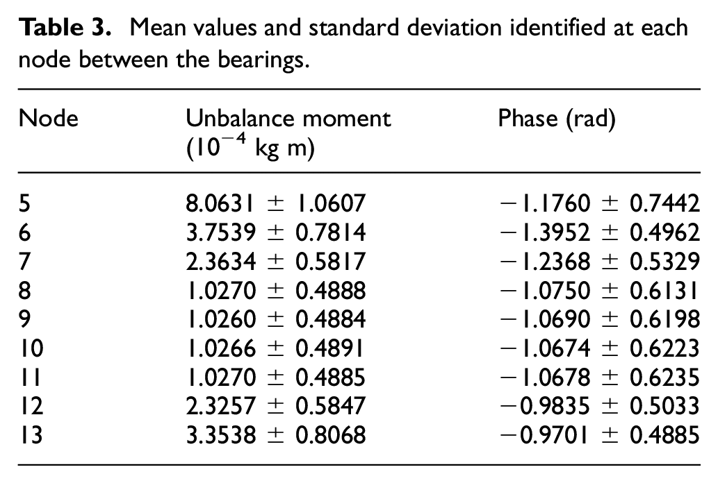
Besides, the value of the objective function for the deterministic identification is 0.3966. In this way, Figure 9 presents the PDFs of the identified parameters at nodes 9–11, which are the most likely nodes for unbalance axial location. Besides the PDF curves, the mean value of the unbalance parameters, as well as the deterministic identification results, are also shown. Table 3 presents the mean values and the standard deviation at all nodes between the bearings (nodes 5–13 of Figure 5), being nodes 10 and 11 highlighted. Despite the high standard deviation values given by the stochastic identifications, mainly due to the influence of the motor coupling effect on bearing 1, both identification and confidence bounds are acceptable in practice, since, in this case, the real values, as well as the deterministic identification, are within two times the standard deviation limits (95% of confidence interval).
Mean values and standard deviation identified at each node between the bearings.
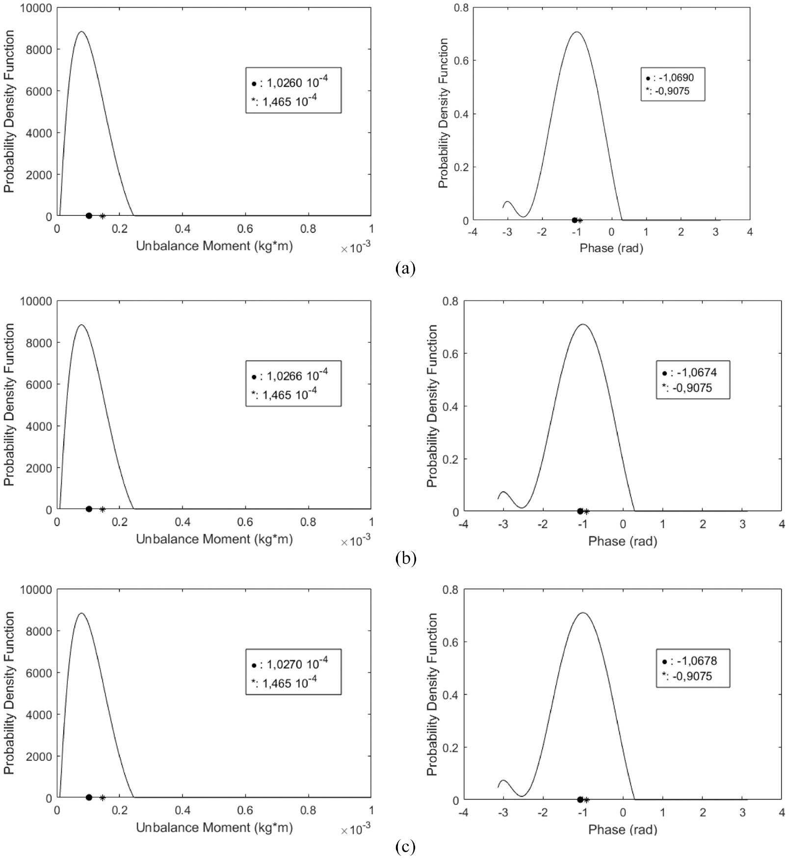
Probability density function of the unbalance moment identified by the Bayesian inference at the nodes 9 (a), 10 (b) and 11 (c).
For the stochastically identified parameters, the uncertainties were quantified according to Figures 10 and 11. Thus, Figure 10 shows a comparison between the experimental (+ marker) and simulation results obtained by the stochastic and deterministic models. The full-line curve represents an average response of the stochastic model, while the dash-dotted line represents the response of the deterministic model (unbalance moment 1.465 × 10⁻⁴ kg m at a phase angle of 308° to the horizontal). The dotted curves represent the upper and lower limits for a 95% confidence interval. Figure 11 emphasizes that the quality of the deterministic identification is influenced by bearing 1, more susceptible to the motor coupling effects. These effects have also influenced the high standard deviation obtained by the stochastic identification since the real unbalance value is known.
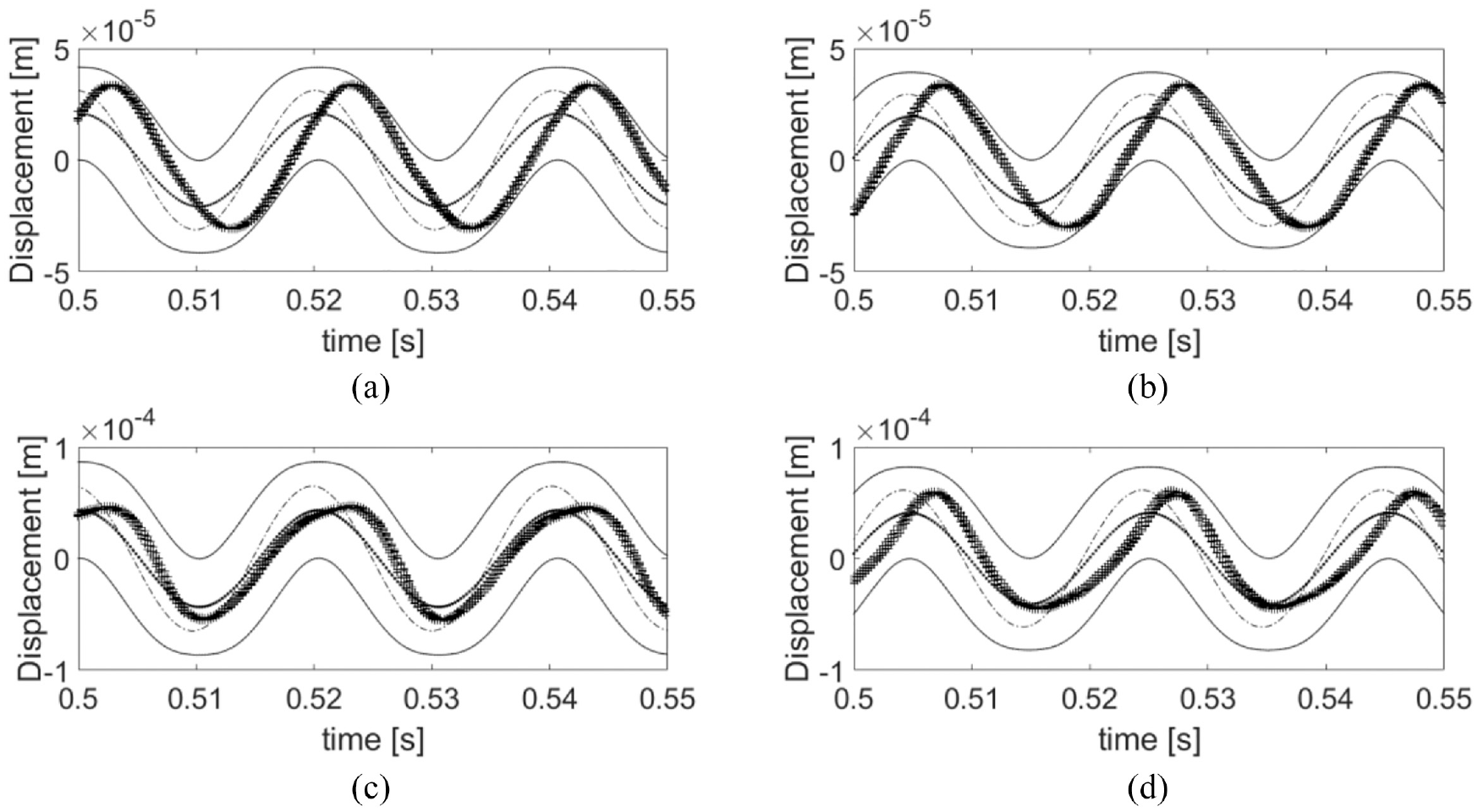
Time response rebuilt with identified parameter for stochastic identification (mean value in dotted line and 95% confidence bounds in full lines), deterministic identification (dash-dot line) and experimental test (+ marker): (a) bearing 1 –y direction, (b) bearing 1 –z direction, (c) bearing 2 –y direction and (d) bearing 2 –z direction.
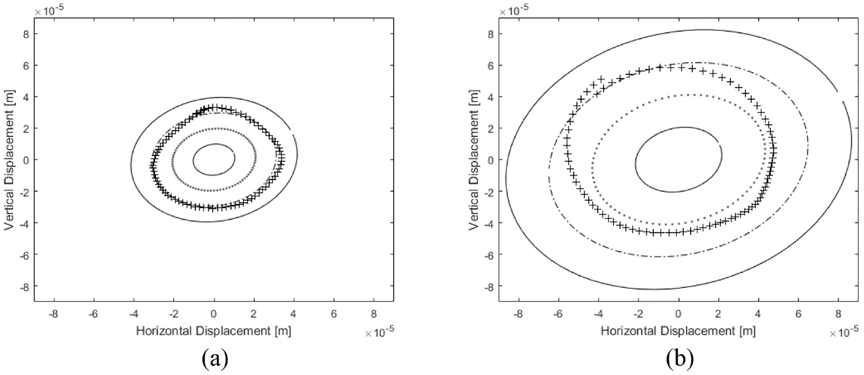
Orbits rebuilt with identified parameter for stochastic identification (mean value in dotted line and 95% confidence bounds in full lines), deterministic identification (dash-dot line) and experimental test (+ marker): (a) bearing 1 and (b) bearing 2.
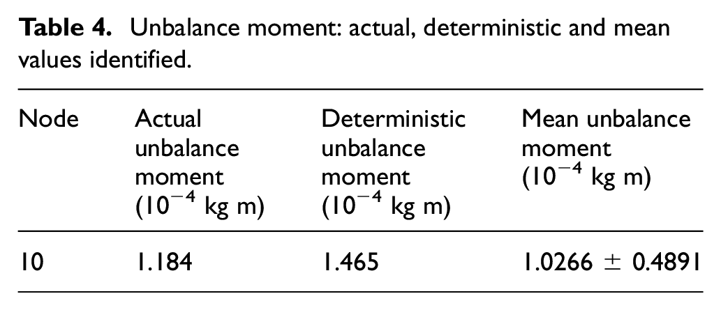
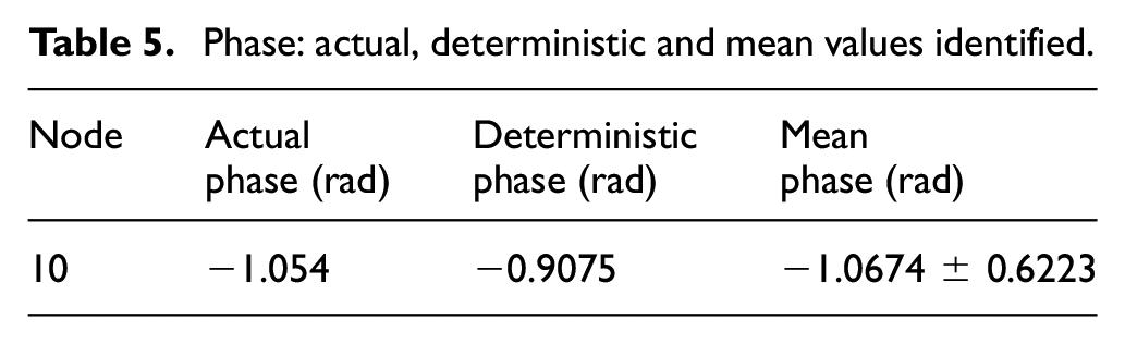
Tables 4 and 5 present the actual unbalance parameters and the identified values for both approaches (deterministic and stochastic). The mean values of the stochastic identification are in good agreement with the actual ones. Besides, it is important to highlight that as the deterministic approach does not take into account any deviation between the real system and the model, the difference between the actual values and the deterministic identification can be a reflection of this assumption.
Unbalance moment: actual, deterministic and mean values identified.
Phase: actual, deterministic and mean values identified.
Another comparison between deterministic and stochastic identifications was accomplished considering the mean values of the stochastic simulation and the deterministic parameter response. In that way, Figures 10 and 11 show the spectrum of both time responses. Figure 12 presents the spectrum amplitudes. The difference between the numerical and experimental response can be quantified by the mean relative error
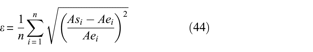
where A is the amplitude of the simulated (s) and experimental (e) signals, and n is the number of points in the frequency range.
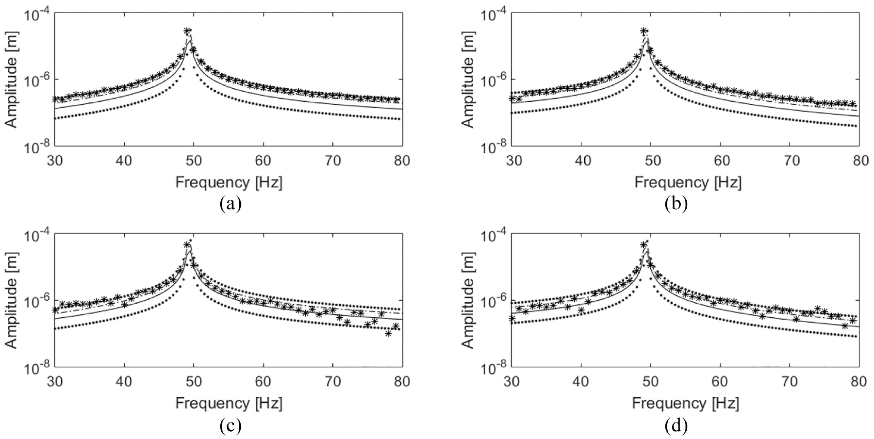
Spectrum of the time response rebuilt with identified parameter for stochastic identification (mean value in full line and 95% confidence bounds in dotted lines), deterministic identification (dash-dot line) and experimental test (+ marker): (a) bearing 1 –y direction, (b) bearing 1 –z direction, (c) bearing 2 –y direction and (d) bearing 2 –z direction.
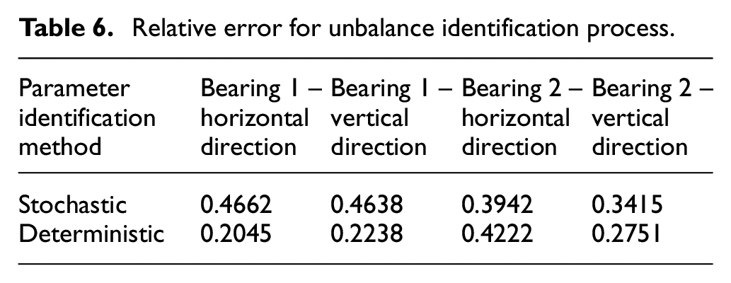
Table 6 shows the relative error
Relative error for unbalance identification process.
Wear identification
The same procedure is accomplished for the bearing wear fault parameters, however using the unbalance response, in directional coordinates, for both model and measurement. It is important to note that the actual wear has depth (d0) of 20.52 µm and its central angular position (γ) is located at 21° from the vertical axis, considering counter-clockwise direction.
Bearing wear faults cause a characteristic change in the backward coordinate of the unbalance response.
15
Therefore, it is possible to consider that the backward direction outweighs the forward direction. Then, to take this fact into account in the Bayesian inference method, it is necessary to set higher values for the weights
The inference was able to identify the marginal posterior distributions for the wear depth and wear angular position. Figures 13 and 14 present both wear identifications as well as the expected wear parameters.
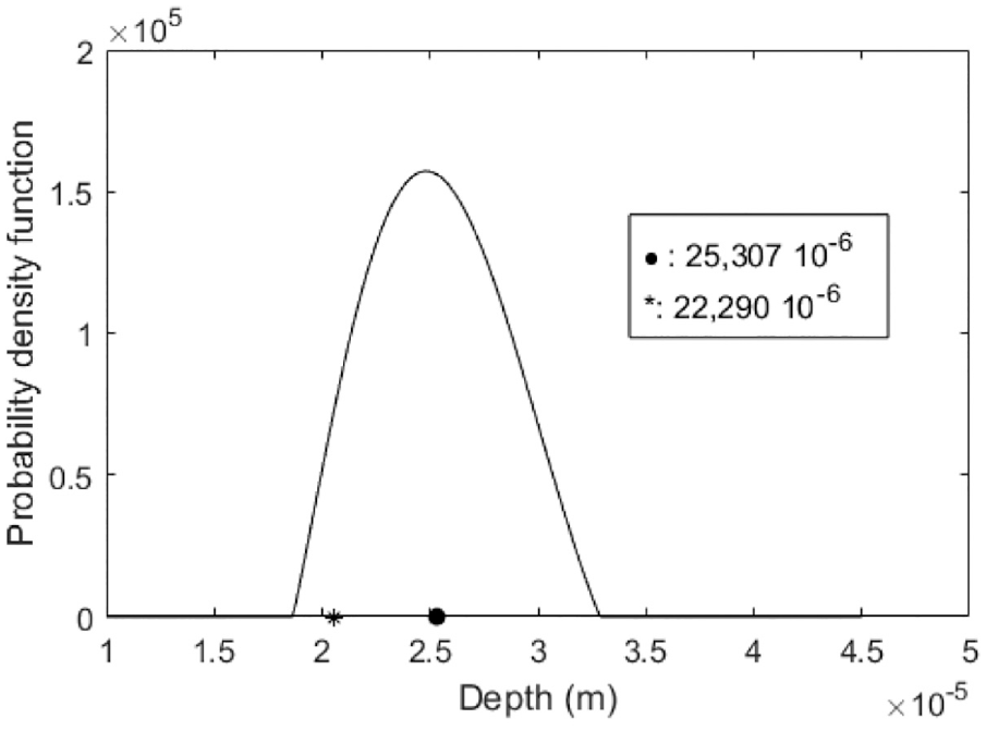
Probability density function of the depth.
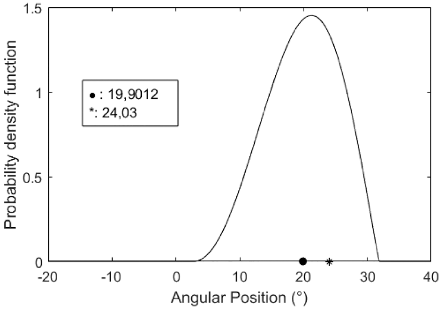
Probability density function of the angular position.
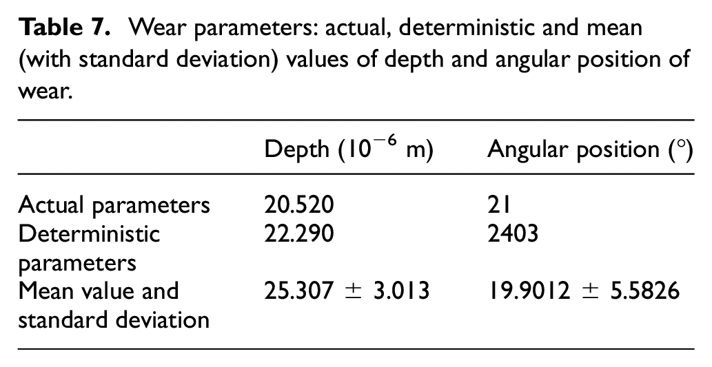
Table 7 shows the mean value and standard deviation of both parameters. As can be seen, both deterministic and stochastic models had some difficulty in finding the exact value of the maximum wear depth, nonetheless achieved a good approximation. For the angular position, the values found by the stochastic model are in better agreement with the real value when compared to the deterministic model.
Wear parameters: actual, deterministic and mean (with standard deviation) values of depth and angular position of wear.
Regarding the quantification of uncertainties compared to the experiment, Figures 15 and 16 show the unbalanced response in the forward and backward coordinates, respectively. These figures consider the experimental results (+), the mean value (full-line curve) of the stochastic response and the confidence interval of 99% (dotted curves). Also, the dash-dotted line represents the response of the deterministic model identification (Table 6).
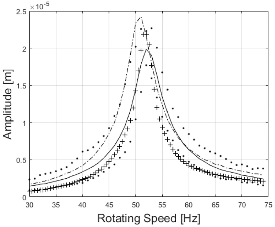
Unbalance response rebuilt in forward precession (mean value in full line and 99% confidence bounds in dotted lines), deterministic identification (dash-dot line) and experimental test (+ marker).
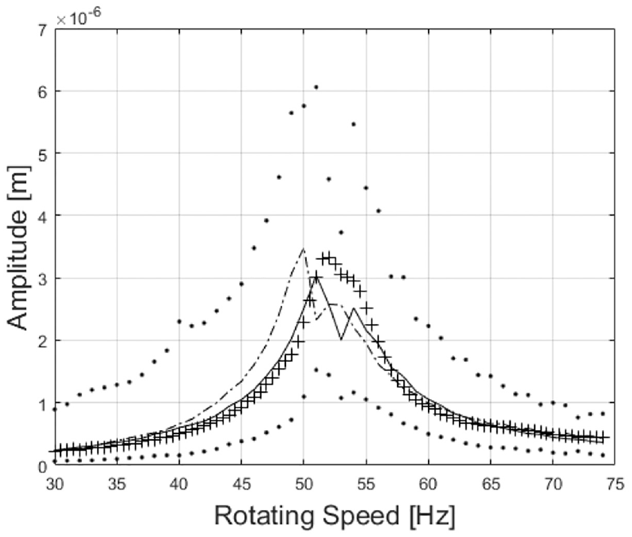
Unbalance response rebuilt in backward precession (mean value in full line and 99% confidence bounds in dotted lines), deterministic identification (dash-dot line) and experimental test (+ marker).
In this case, both rebuilt curves are in good agreement with the experimental measurements due to the wear parameters estimated (Table 7). This fact is a consequence of the scaling applied to the backward response, which is the most important information regarding the anisotropic effects increased due to bearing wear presence.
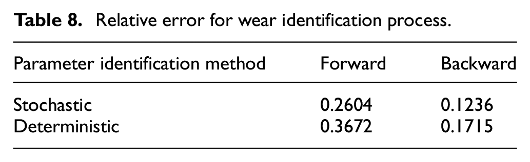
Again, a new comparison between both results (experimental and numerical) was accomplished. The amplitudes in Figures 15 and 16 are considered, as well as the relative error
Relative error for wear identification process.
Conclusion
Two characteristic fault models of rotating machines supported by lubricated bearings were investigated regarding their main parameter identification and under two points of view: deterministic and stochastic approaches. The MINLP is applied for the deterministic identification process of three unbalance parameters, namely, unbalance moment, phase and the axial location at the shaft, as well as two wear parameters: depth and angular position in the bearing. The same parameters are also identified by the Bayesian inference with polynomial chaos expansion to quantify the uncertainties involved in each parameter and, consequently, its quantification in the rebuilt system response.
Both approaches are promising for the application proposed here. However, the stochastic one can also give the deviation either on the identified parameters or on the system response.
It is important to note that in both fault cases, the bound limits involved the measured response and the rebuilt curve from the deterministic identification with high confidence limits of 95% for rotor unbalance and 99% for bearing wear. Another point to be highlighted is that the stochastic approach is obtained from the mean value, instead of the highest probability density value, reinforcing the promising application of polynomial chaos expansion in the Bayesian inference identification, besides the complexity of rotating machinery system modelling and dynamic analysis.
Finally, it can be concluded that the main novelty of this article is the use of polynomial chaos expansion technique employed along with identification via the Bayesian inference, in order to accelerate the identification process, via models (model-based identification), of fault parameters in rotating machines, since in general, models for these components demand high-computational processing time.
Footnotes
Declaration of conflicting interests
The author(s) declared no potential conflicts of interest with respect to the research, authorship and/or publication of this article.
Funding
The author(s) disclosed receipt of the following financial support for the research, authorship and/or publication of this article: This work was supported by the FAPESP (grant numbers 2015/20363-6, 2016/13223-6, 2018/21581-5 and 2018/24600-0) and the CNPq (grant no. 307941/2019-1).