A novel model-based unbalance monitoring and prognostics for rotor-bearing systems

Abstract

A novel model-based unbalance monitoring and prognostics for rotor-bearing systems is introduced in the paper. An analytical method is first applied for rotor modeling and the calculated first natural frequency is validated by an FEM model. The rotor-bearing model with the identified bearing parameters is next validated with an operational 3-stage turbine-bearing’s machine on the first critical speed. The novelty of the approach is that the unbalance proceeding with optimization schemes is evaluated in two phases. In phase I, the bearing parameters and the initial unbalances are simultaneously evaluated based on the operational data soon after an overhaul. In phase II, the unbalance deterioration with time is identified through every day’s measured vibration at two bearings. A set of operational data over 16 months, provided by a local company, are used to test the approach. The evaluated unbalance deterioration trend is verified by the collaborated company from two consecutive overhauls. Five optimization algorithms are also tested and the results prove the robustness of the derived approach. Finally, the unbalance forecasting capability extrapolating from historical unbalance curve is demonstrated and that can work as prognostics in a condition-based maintenance strategy.

Introduction

To achieve the goal of higher operational reliability and lower maintenance cost the maintenance strategy has evolved from corrective (unscheduled, passive), preventive (scheduled, active), to condition-based (predictive, proactive) maintenance (CBM). ¹ The success of CBM relies on appropriate monitoring approaches and faults diagnostic algorithms. Conventional monitoring approaches monitor operational variables like pressure, temperature, vibration and set alarms if certain limits are exceeded. These approaches, in general, do not give a deeper insight and mostly detect machine faults at a rather late stage. ² The tendency toward earlier faults detection and identification has driven researchers to continuously develop advanced techniques of monitoring and diagnosis. For years, the success of monitoring systems has brought benefits to the industry. The requirement for ever increasing operation time and decreasing unscheduled downtime, however, posts extra challenges for research and industry. Nowadays, diagnosis of a rotor fault before it becomes critical is still the greatest challenge in condition monitoring of machinery. ³

Rotating machinery usually plays an important role in petrochemical and power generation plants. Failure of any rotating element brings safety implications along with economic concerns. Hence, continuous fault-monitoring in rotating machinery has been demanding for decades. The foundation of faults monitoring and diagnosis in rotating machinery is the vibration variations, which are very sensitive to small structure variations as well as changes in the process parameters. Any fault occurred in a rotor will affect its vibration behavior and the nature of this effect is mostly dependent on different types of faults. In light of this, vibration-based diagnosis (VBD) has become well accepted and widely applied in practice to identify a wide range of rotor faults. ⁴ Walker et al. ⁵ reviewed the recent advances in vibration-based diagnosis and prognosis of rotors with common faults in which the approaches can be data-driven, model-based, or the combination of two, that is, hybrid.

Data-driven approaches make use of information from a bunch of collected data and employ statistical models for fault diagnosis. With the advancement in signal processing techniques such as wavelet transforms,^6–8 empirical mode decomposition (EMD) and Hilbert–Huang transforms (HHT),^9–11 data-driven approaches incorporated with artificial intelligent (AI) techniques have become and will remain popular and promising in the foreseeable future. Liu et al. ¹² presented a comprehensive review of AI algorithms applied to rotating machinery fault diagnosis from the aspects of theoretical development and industrial applications. In that paper, various examples on application to rotor diagnostics were illustrated, such as k-Nearest neighbor for bearing’s fault, ¹³ Naïve Bayes classifier for induction motor’s fault, ¹⁴ support vector machine (SVM) for rotor’s multi-fault, ¹⁵ artificial neural network (ANN) for gearbox, ¹⁶ shaft lateral crack, ¹⁷ bearing fault, ¹⁸ and deep learning ¹⁹ for rotating machinery diagnosis. Data-driven approaches, in general, make no attempt to derive the Physics underlying the rotor systems and hence are useful for data interpolation but uncertain for extrapolation results. ⁴ The advantages of data-driven approaches are no need to derive physical models of rotors and the vibration data can quickly provide early indication of fault-occurrence. The diagnosis of rotor faults entirely relying on the measured data, however, is limited to qualitative symptoms. Quantification of faults, such as unbalance severity (location and amount), usually requires substantial plant testing which may be very time-consuming, if not impossible.

Model-based methods emanating from physical model (full or partial) of rotor systems, on the other hand, have the vantage of faster and more accurate faults quantification. In addition, the results obtained by models are usually physically interpretable. Lees et al. ⁴ gave a detailed review on the use of model-based fault-identification methods for rotating machines. Those model-based approaches although have their own merits, they basically follow very similar procedures: generation of residuals, diagnosis, and isolation of faults. ²⁰ For instance, Bachschmid et al. ²¹ proposed a method for multi-fault identification by means of minimizing a multi-dimensional residual between the measured vibrations and calculated ones due to acting faults. Bachschmid and Pennacchi ²² used the residual as a qualitative index to evaluate the accuracy of the performed identification and it has been widely adopted thereafter.

Regarding the faults existing in rotating machinery, there are eight commonly acknowledged faults: unbalance, shaft bow, coupling misalignment, rub, looseness, fluid-induced instabilities, bearing faults, and cracks. ²³ Among these faults, three of them stand alone and emerge in the initial phase. They are unbalance, misalignment, and shaft bows. ²⁴ Although the common faults have been categorized into eight types, they are by no means mutually exclusive. Dependencies often exist among many of them. The process of multi-fault diagnosis is hence more complex than that of a single fault. Jing and Meng ²⁵ proposed a blind source separation method for multi-fault diagnosis of rotor system and proved its feasibility from simulation and experiments. Zhang et al. ²⁶ employed a lumped dynamic model together with an improved EMD technique to investigate a rotor-bearing system with three types of faults, unbalance, misalignment, rub-impact, and the coupling of them. Jalan and Mohanty ² developed an FEM model-based fault diagnosis technique for identifying unbalance and misalignment of a rotor-coupling-bearing system under a steady-state condition. By minimizing the error between measured and calculated forces under an optimization algorithm they separately identified the unbalance and the misalignment. This method is, in a sense, based on parameter estimation and parity equations. ²⁷

Unbalance has been acknowledged as the most common and primary fault in rotor systems since every rotating element has an inherent degree of unbalance due to material and geometrical imperfection, tolerance of mating parts, and assembling errors. Therefore, unbalance identification has been studied for decades. Sudhakar and Sekhar ³ developed a model-based unbalance identification approach in a rotor-bearing system using two different optimization criteria: equivalent loads minimization and vibration minimization. They identified the unbalance and experimentally validated it from a test rig. They concluded that vibration minimization approach has less error than the equivalent loads minimization one. Yao et al. ²⁸ proposed an integrated modal expansion/inverse problem combined with an optimization procedure to minimize the error at unmeasurable points and identify the unbalance. Michalski and de Souza ²⁴ applied a Karman filter method for unbalance estimation and validated their results with two cases: a test rig and a real turbocharger. Most of the model-based unbalance identification methods work under steady operation, that is, constant rotational speed. Zhao et al. ²⁹ developed a transient balancing technique, in which the coordinate transformation, modal analysis and FEM were employed to identify unbalance parameters. They calculated the transient excitation forces based on the transient responses and modal parameters at specific positions. The unbalance parameters were then identified using the calculated excitation forces. The accuracy and robustness of the approach was shown by numerical simulations and experiments on a test rig.

Most of the model-based fault-identification methods assume known bearing parameters. Nonetheless, proper evaluation of bearing parameters in a rotor-bearing system is deemed a crucial and important step prior to unbalance identification. The evaluation of bearing parameters can be achieved using optimization schemes integrated with the measured response, either from test rigs or real operational machines. Taking a hydrodynamic bearing as an instance, its dynamic parameters are functions of speed, eccentric ratio, and other variables so that their estimation usually requires elaborate works. Mutra and Srinivas ³⁰ employed a FEM model for a rotor-bearing system and used an error-based formulation in terms of response amplitudes at bearing nodes to identify the speed-dependent stiffness and damping parameters of a hydrodynamic bearing, in which a modified particle swarm optimization (PSO) with mutation was applied for solution search. The robustness of the methodology was confirmed via introducing different levels of noise into the measured reference signals.

A hydrostatic bearing usually has a much smaller eccentric ratio therefore the main factors that could affect the bearing stiffness and damping coefficients are the supplied lubricant’s pressure and temperature, which are usually controlled to vary in a relatively small range. Martin ³¹ experimentally measured the stiffness of a hydrostatic bearing and compared with the published empirical guidelines. He concluded that the direct and cross stiffness coefficients can be assumed constant for a range of load and oil supply pressure. It is hence reasonable to assume the coefficients of a hydrostatic bearing to be constants for analytical simplicity. As to the evaluation of those coefficients, it is not suggested to fully follow pure calculations according to either theoretical or empirical equations, because the bearing coefficients are very sensitive to film thickness, alignment, and assembly tolerance etc., which inevitably vary at every assembly. Mao et al. ³² derived an analytical model of a rotor-bearing using transfer matrix method and characterized the bearing parameters by minimizing the error of unbalance response between the experimental results of a test rig and their computational counterparts. Kang et al. ³³ presented an FEM model to update the bearing stiffness matrix of a rotor-bearing system via the PSO algorithm when the shaft was not rotating (structure testing). Validation of the updated results was performed by comparing the frequency spectrum of the model with that of an experiment. The results show the updated model indeed resembles the test rig better than the original one.

The mentioned model-based papers above identified either the unbalances or bearing parameters, separately. Research reports that simultaneously estimated bearing parameters and unbalances together are relatively limited. Analytical methods to simultaneous identification of unbalance and bearing parameters usually require applying external forces, test runs, or varying speeds. Tiwari and Chakravarthy, ³⁴ one of the typical works, simultaneously estimated the residual unbalance and bearing parameters from the experimental data of a rotor-bearing system, in which the data were obtained from the impulsive response and the rundown test of a rig. Their results show the identified unbalance masses match the residual masses taken in the rotor-bearing test rig. In their model, however, the shaft-disk was treated as a single rigid assembly, whereas the system’s stiffness solely came from the bearings. To the authors’ opinion, the rigid shaft-disk assumption is appropriate only if the rotor runs far below its first critical speed. If the rotor-bearing runs far above its first critical speed the shaft’s flexibility would significantly contribute to the total vibration response and cannot be ignored. Recently, Wang et al. ³⁵ analytically derived an algorithm for simultaneous identification of residual unbalance and bearing dynamic coefficients of a single-disk and single-span rotor using Rayleigh’s beam model. In that paper, the flexibility of shaft is considered, and the algorithm requires no external forces or test runs. The identification process is in three steps: First, the identification of unbalance; Second, the identification of bearing coefficients; And the lastly, simultaneous identification of unbalance and bearing coefficients is derived. In each step, it requires measurements at plate and specific shaft cross-sections. To the last, it needs only the responses at two-bearing and disk locations to simultaneously identify the unbalance and bearing coefficients.

In spite of that unbalance identification has been studied for so many years, continuous unbalance monitoring and prognostics still issues a unique set of challenges ⁵ and stay as a limited area of investigation. ²⁴ Prognosis of rotor unbalance is difficult to specify the so-called remaining useful life (RUL) because complicated factors, such as fault dependencies, are frequently involved in the rotor unbalance deterioration. In many cases the unbalance itself is not the main failing factor. For instance, the growth of unbalance may result in looseness of machine parts or a rub event, which eventually leads to the final damage. Due to the fact that rotor unbalance is usually the primary vibration source and could induce many other types of faults that would lead to rotor failure, monitoring the rotor’s unbalance in an online and real-time base is valuable to the current CBM strategy. In view of that, the present research aims to develop a model-based online unbalance monitoring and prognostic algorithm eligible for rotor-bearing systems. In the very recent, Puerto-Santana et al. ³⁶ derived a continuous unbalance monitoring approach using the Jeffcott rotor model. Techniques of signal processing are applied for response data and subspace identification method is used for model matrices identification. To the end, the unbalances in rotating machinery can be estimated.

The novelty of the present approach is two-phase parameter identification. In phase I, the bearing parameters and initial unbalances at two bearing planes right after an overhaul are simultaneously evaluated similar to Tiwari and Chakravarthy ³⁴ but the shaft is treated flexible here. Afterward, the bearing parameters are kept unchanged (unless the rotor is subject to disassembly, then the bearings’ parameters need to be reevaluated) while the progression of unbalances on a daily base is evaluated in phase II. Diagnosis in terms of static and dynamic unbalance can then be characterized, and a feasible way for unbalance prognosis/forecast is proposed. To the authors’ knowledge, the methodology derived in the present paper has not been seen in the published literature.

The structure of the paper is organized as the follows. In section 2, the methodology and flowchart is outlined so that a clear picture of the approach can be easily visualized; Section 3 describes the mathematical models, where 3.1 is for turbine-bearing rotor and 3.2 is for hydrostatic bearing; Section 4 describes details regarding data acquisition and features selection; Section 5 presents the process of parameter identification, in which optimization algorithms are described in 5.1 while model validation is given in 5.2; Section 6.1 demonstrates the context of unbalance progression estimation and the forecasting model for prognosis is introduced in 6.2; Finally, concluding remarks are drawn in section 7.

Methodology and process

The methodology and its process for monitoring and prognostics of rotor-bearing unbalance is illustrated in Figure 1. Since rotating machinery often plays the key role in the production line of petrochemical plants, run-to-failure data are very limited. Data-driven approaches to rotor fault diagnostics/prognostics using insufficient training data set to yield digital models, such as artificial neural networks (ANN), are considered dangerous and impractical. Physical modeling employing domain knowledge provides an alternative to overcome data shortage. This is the motive of the present research. The derived approach begins with the physical and mathematical models of rotor and bearing. The rotor model with rigid supports is first validated by an FEM model on its first natural frequency. Parameter identification in two phases then follows to estimate the bearing parameters and unbalances. In phase I, as the bearings’ parameters are identified, the rotor-bearing combination is further validated with the operational data on its first critical speed. Progression of unbalances are estimated in phase II. Unbalance in terms of static and dynamic quantities are also evaluated and robustness of the approach is examined. Finally, the unbalance prognostics is proposed.

Figure 1.

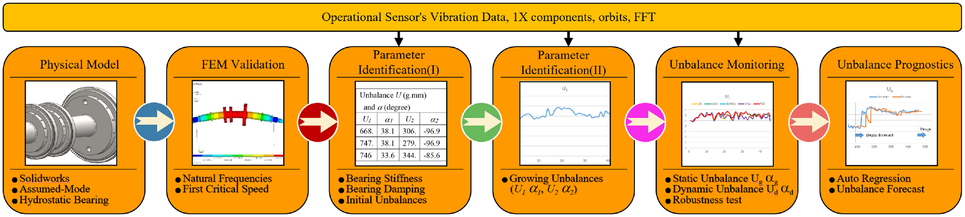
The methodology for monitoring/prognostics of rotor-bearing unbalance.

Physics-based models

Figure 2 shows the schematic diagram of the turbine-bearing system under investigation, where Figure 2(a) shows the geometric dimensions and coordinates, Figure 2(b) displays the 3D model generated by Solidworks, and Figure 2(c) is the first natural mode obtained by FEM. The turbine-bearing system consists of a flexible shaft, a 3-stage impeller, and two 5 tilting-pad hydrostatic fluid-film bearings near shaft’s ends. The rotor system runs at an operational speed near 11,000 rpm. However, it is balanced at a rather low speed around 600 rpm in each overhaul. That implies the rotor is treated as quasi-flexible, that is, the shaft’s deformation is not considered in overhaul balancing.

Figure 2.

Schematic diagram of turbine-bearing rotor, (a) dimensions and coordinates, (b) Solidworks formation, and (c) FEM model of the first natural mode.

Mathematic model of turbine-bearing rotor

Most of model-based approaches develop the rotor model via FEM. The present one, instead, employs the assumed-mode method (AMM) for equations of motion (EOMs). The reason of not using a commercial FEM software is that, on one hand, the investigated rotor is homogeneous with simple geometry. A general, commercial FEM code seems redundant and inefficient in computation. On the other hand, the derived approach is to be installed in an in-situ monitoring system for online and real-time unbalance estimation at a local company, where FEM software is unavailable. Nonetheless, FEM results of the first natural mode obtained in laboratory, as shown in Figure 2(c), is used to validate those obtained from the assumed-mode method. The natural frequencies obtained from both models agree with each other with a difference less than 2% (84.4 vs 83.0 Hz), under the rigid support condition. Note that the bearing effect is not considered in this moment. When fluid-film bearings properties are identified, the combination of turbine-bearing will be validated according to operational data so that the derived model will more closely represent the actual system. Note that the blades vibration mostly affects the shaft’s torsional and axial behavior not the bending so the disk-blade is considered as a single rigid element in the present model.

Based on AMM, the displacements of rotor’s center line in x and y directions, measured with respect to the stationary coordinates, can be expressed as u(z,t) and v(z,t),

$$u(z,t)={\sum }_{i=1}^m{p}_i(t){\Phi }_i(z)={\mathit{p}}^T\mathit{\Phi },$$

(1)

$$v(z,t)={\sum }_{i=1}^m{q}_i(t){\Phi }_i(z)={\mathit{q}}^T\mathit{\Phi }.$$

(2)

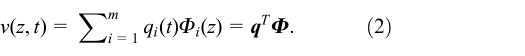
where the assumed modes, Φ _i (z)’s, consist of the natural modes of a free-free beam plus two rigid body modes, translation and rotation. p and q are the so-called generalized coordinates. m is the number of modes deemed necessary accuracy. It has been tested that m =6 (including rigid-body modes) is enough to converge the first natural frequency to the first decimal digit. The EOMs, via the Lagrange’s equation, are derived to be

$$\begin{array}{c}\left[\begin{array}{cc}\mathit{M}+\mathit{N}\hfill & 0\hfill \\ \multicolumn{1}{c}{0}& \mathit{M}+\mathit{N}\hfill \end{array}\right]\left\{\begin{array}{c}\stackrel{··}{\mathit{p}}\hfill \\ \multicolumn{1}{c}{\stackrel{··}{\mathit{q}}}\end{array}\right\}+\left[\begin{array}{cc}{\mathit{C}}_x\hfill & 2\mathrm{\Omega }\mathit{N}\hfill \\ \multicolumn{1}{c}{-2\mathrm{\Omega }\mathit{N}}& {\mathit{C}}_y\hfill \end{array}\right]\left\{\begin{array}{c}\stackrel{·}{\mathit{p}}\hfill \\ \multicolumn{1}{c}{\stackrel{·}{\mathit{q}}}\end{array}\right\}\hfill \\ +\left[\begin{array}{cc}{\mathit{K}}_x-{\mathrm{\Omega }}^2\mathit{N}\hfill & 0\hfill \\ \multicolumn{1}{c}{0}& {\mathit{K}}_y-{\mathrm{\Omega }}^2\mathit{N}\hfill \end{array}\right]\left\{\begin{array}{c}\mathit{p}\hfill \\ \multicolumn{1}{c}{\mathit{q}}\end{array}\right\}=\left\{\begin{array}{c}{\mathit{Q}}_x\hfill \\ \multicolumn{1}{c}{{\mathit{Q}}_y}\end{array}\right\}\hfill \end{array}$$

(3)

$$M_{\mathrm{ij}}={\int }_0^l\rho A{\Phi }_i(z){\Phi }_j(z)\mathrm{dz}+{\sum }_{r=1}^{n_d}{m}_r^d{\Phi }_i(z_r){\Phi }_j(z_r)$$

(4)

$$N_{\mathrm{ij}}={\int }_0^l\rho I_A{\Phi }_i\prime (z){\Phi }_j\prime (z)\mathrm{dz}+{\sum }_{r=1}^{n_d}{I}_r^d{\Phi }_i\prime (z_r){\Phi }_j\prime (z_r)$$

(5)

$$C_{x_{\mathrm{ij}}}={\sum }_{n=1}^{n_b}{C}_{\mathrm{xn}}{\Phi }_i(z_n){\Phi }_j(z_n)$$

(6)

$$C_{y_{\mathrm{ij}}}={\sum }_{n=1}^{n_b}{C}_{\mathrm{yn}}{\Phi }_i(z_n){\Phi }_j(z_n)$$

(7)

$$K_{x_{\mathrm{ij}}}={\int }_0^{l}E{I}_A{\Phi }_i\prime \prime (z){\Phi }_j\prime \prime (z)\mathrm{dz}+{\sum }_{n=1}^{n_b}{k}_{\mathrm{xn}}{\Phi }_i(z_n){\Phi }_j(z_n)$$

(8)

$$K_{y_{\mathrm{ij}}}={\int }_0^{l}E{I}_A{\Phi }_i\prime \prime (z){\Phi }_j\prime \prime (z)\mathrm{dz}+{\sum }_{n=1}^{n_b}{k}_{\mathrm{yn}}{\Phi }_i(z_n){\Phi }_j(z_n)$$

(9)

where $(\stackrel{·}{})=d/\mathrm{dt},(\prime )=d/\mathrm{dz}$ . M, N, C, and K, respectively, represent the mass, rotary inertia, damping, and stiffness matrix. n_d, m^d, I^d, n_b, and I_A denote the number of disks, disk’s mass, disk’s diametric inertia, number of bearings, and shaft’s area moment of inertia, respectively. From equations (8) and (9), it is seen the system’s total stiffness comprises the shaft and the fluid-film bearings, but the system’s damping is solely due to fluid-film bearings because the structure damping in shaft is neglected. Ω denotes the rotational speed in rad/s and Q_x,Q _y are the so-called generalized force vectors. Note that he measured vibration amplitudes at all sensors have been inspected and found that all readings are in a range of just a few micrometers. Based on these observations a linear model like equation (3) would be precise enough for the studied case.

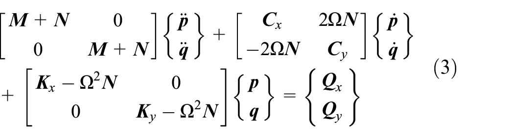
The unbalance forces/moments exerted on a running rotor, in nature, are distributed over the whole shaft length, but they can always be lumped together and located at specific points such as the mass center, balancing disks, or bearings’ locations. In the following, the derivation due to one single unbalance locating at the gravity center is demonstrated. For multi-point unbalances, the principle of superposition can be applied for the total response. The unbalanced (centrifugal) forces when decomposed into x and y components can be expressed as

$$F_x=U_g{\mathrm{\Omega }}^2\cos (\mathrm{\Omega }t+{\alpha }_g)\delta (z-z_g),$$

(10)

$$F_y=U_g{\mathrm{\Omega }}^2\sin (\mathrm{\Omega }t+{\alpha }_g)\delta (z-z_g)$$

(11)

where U_g=(me) is the customarily specified unbalance with a unit of gmm, α _g is the unbalance phase angle relative to the key phasor, and δz) is the Dirac delta function used to locate a concentrated force. Here, the subscript g denotes the gravity center. The generalized force vectors in equation (3) are accordingly calculated to be

$$\begin{array}{c}\multicolumn{1}{c}{{\mathit{Q}}_x=U_g{\mathrm{\Omega }}^2\cos {\alpha }_g\mathit{\Phi }(z_g)\cos (\mathrm{\Omega }t)-U_g{\mathrm{\Omega }}^2\sin {\alpha }_g\mathit{\Phi }(z_g)\sin (\mathrm{\Omega }t)}\\ ={\mathbf{F}}_c(z_g)\cos (\mathrm{\Omega }t)-{\mathit{F}}_s(z_g)\sin (\mathrm{\Omega }t)\hfill \end{array}$$

(12)

$$\begin{array}{c}\multicolumn{1}{c}{{\mathit{Q}}_y=U_g{\mathrm{\Omega }}^2\sin {\alpha }_g\mathit{\Phi }(z_g)\cos (\mathrm{\Omega }t)+U_g{\mathrm{\Omega }}^2\cos {\alpha }_g\mathit{\Phi }(z_g)\sin (\mathrm{\Omega }t)}\\ ={\mathbf{F}}_s(z_g)\cos (\mathrm{\Omega }t)+{\mathit{F}}_c(z_g)\sin (\mathrm{\Omega }t)\hfill \end{array}$$

(13)

where ${\mathit{F}}_c(z_g)=U_g{\mathrm{\Omega }}^2\cos {\alpha }_g\mathit{\Phi }(z_g)\mathrm{and}{\mathbf{F}}_s(z_g)=U_g{\mathrm{\Omega }}^2\sin {\alpha }_g\mathit{\Phi }(z_g)$ , denoted with self-explanatory subscripts, represent the cosine and sine component vector of the generalized force, respectively. Substituting equations (12) and (13) into equation (3), the cosine and sine components of the generalized coordinates, denoted p _c , q _c and p _s , q _s , respectively, can be solved from the following equations,

$$\begin{array}{c}\left[\begin{array}{cccc}{\mathit{K}}_x-{\mathrm{\Omega }}^2\mathit{M}-2{\mathrm{\Omega }}^2\mathit{N}\hfill & \mathrm{\Omega }{\mathit{C}}_x\hfill & 0\hfill & 2{\mathrm{\Omega }}^2\mathit{N}\hfill \\ \multicolumn{1}{c}{-\mathrm{\Omega }{\mathit{C}}_x}& {\mathit{K}}_x-{\mathrm{\Omega }}^2\mathit{M}-2{\mathrm{\Omega }}^2\mathit{N}\hfill & -2{\mathrm{\Omega }}^2\mathit{N}\hfill & 0\hfill \\ \multicolumn{1}{c}{0}& -2{\mathrm{\Omega }}^2\mathit{N}\hfill & {\mathit{K}}_y-{\mathrm{\Omega }}^2\mathit{M}-2{\mathrm{\Omega }}^2\mathit{N}\hfill & \mathrm{\Omega }{\mathit{C}}_y\hfill \\ \multicolumn{1}{c}{2{\mathrm{\Omega }}^2\mathit{N}}& 0\hfill & -\mathrm{\Omega }{\mathit{C}}_y\hfill & {\mathit{K}}_y-{\mathrm{\Omega }}^2\mathit{M}-2{\mathrm{\Omega }}^2\mathit{N}\hfill \end{array}\right]\left\{\begin{array}{c}{\mathit{p}}_c\hfill \\ \multicolumn{1}{c}{{\mathit{p}}_s}\\ \multicolumn{1}{c}{{\mathit{q}}_c}\\ \multicolumn{1}{c}{{\mathit{q}}_s}\end{array}\right\}\hfill \\ =\left\{\begin{array}{c}{\mathit{F}}_c\hfill \\ \multicolumn{1}{c}{-{\mathit{F}}_s}\\ \multicolumn{1}{c}{{\mathit{F}}_s}\\ \multicolumn{1}{c}{{\mathit{F}}_c}\end{array}\right\}\hfill \end{array}$$

(14)

Equation (14) gives us the complete solution to an unbalance excitation wherein the rotary inertia, bearing asymmetry and Coriolis forces have all been considered. If the rotary inertia N and subsequently the Coriolis terms have been neglected equation (14) would reduce to

$$\left[\begin{array}{cc}{\mathit{K}}_x-{\mathrm{\Omega }}^2\mathit{M}\hfill & \mathrm{\Omega }{\mathit{C}}_x\hfill \\ \multicolumn{1}{c}{-\mathrm{\Omega }{\mathit{C}}_x}& {\mathit{K}}_x-{\mathrm{\Omega }}^2\mathit{M}\hfill \end{array}\right]\left\{\begin{array}{c}{\mathit{p}}_c\hfill \\ \multicolumn{1}{c}{{\mathit{p}}_s}\end{array}\right\}=\left\{\begin{array}{c}{\mathit{F}}_c\hfill \\ \multicolumn{1}{c}{-{\mathit{F}}_s}\end{array}\right\}$$

(15)

$$\left[\begin{array}{cc}{\mathit{K}}_y-{\mathrm{\Omega }}^2\mathit{M}\hfill & \mathrm{\Omega }{\mathit{C}}_y\hfill \\ \multicolumn{1}{c}{-\mathrm{\Omega }{\mathit{C}}_y}& {\mathit{K}}_y-{\mathrm{\Omega }}^2\mathit{M}\hfill \end{array}\right]\left\{\begin{array}{c}{\mathit{q}}_c\hfill \\ \multicolumn{1}{c}{{\mathit{q}}_s}\end{array}\right\}=\left\{\begin{array}{c}{\mathit{F}}_s\hfill \\ \multicolumn{1}{c}{{\mathit{F}}_c}\end{array}\right\}$$

(16)

It is seen p and q are uncoupled and can be separately solved for. In addition, the left-hand sides of equations (15) and (16) will be identical such that p _c  =  q _s , p _s  = −q _c if the turbine-bearing rotor is symmetric in x-y direction. This attribute can be used for data-validity check as the rotor runs at low speed (transient), wherein the rotary inertia and Coriolis are negligible and equations (15) and (16) should be approximately satisfied. In steady operation, the rotor runs far above its first critical speed and equation (14) is suggested for more accurate solution. It is worth mentioning that a rotor may be intentionally designed symmetrical, but its real behavior is rarely symmetric because of weight distribution, inherent material inhomogeneity, geometric imperfection, bearing asymmetry, and loading condition etc.

The rotor’s unbalance responses in x and y directions, after solving equation (14), can be expressed as

$$\begin{array}{c}\multicolumn{1}{c}{u(z,t)={\mathit{p}}_c^{\mathrm{T}}\mathit{\Phi }(z)\cos (\mathrm{\Omega }t)+{\mathit{p}}_s^{\mathrm{T}}\mathit{\Phi }(z)\sin (\mathrm{\Omega }t)}\\ =u_c(z)\cos (\mathrm{\Omega }t)+u_s(z)\sin (\mathrm{\Omega }t)=A_x\cos (\mathrm{\Omega }t-{\varphi }_x)\hfill \end{array}$$

(17)

$$\begin{array}{c}\multicolumn{1}{c}{v(z,t)={\mathit{q}}_c^{\mathrm{T}}\mathit{\Phi }(z)\cos (\mathrm{\Omega }t)+{\mathit{q}}_s^{\mathrm{T}}\mathit{\Phi }(z)\sin (\mathrm{\Omega }t)}\\ =v_c(z)\cos (\mathrm{\Omega }t)+v_s(z)\sin (\mathrm{\Omega }t)=A_y\cos (\mathrm{\Omega }t-{\varphi }_y)\hfill \end{array}$$

(18)

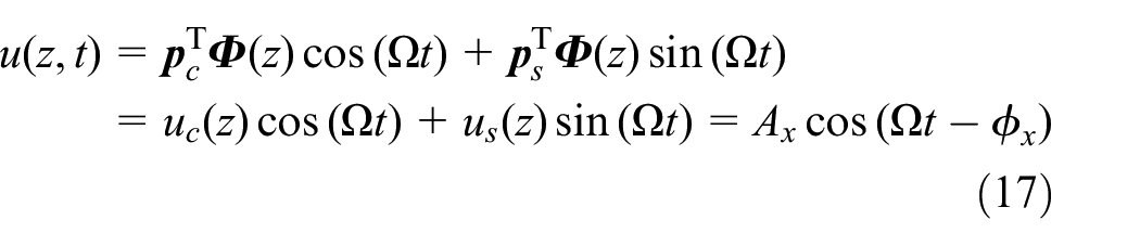
Equations (17) and (18) are the calculated unbalance vibration, and they play the key role in the following parameters identification. The 1x components out of sensors’ measured response will be extracted and compared against the calculations from equations (17) and (18) to generate the residual. Employing optimal schemes to minimize the residual will yield the most suitable model parameters, including bearing parameters and unbalances.

Mathematic model of hydrostatic bearing

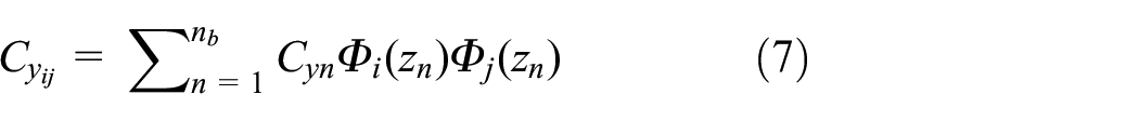
The turbine under investigation is supported by two 5 tilting-pad, fluid-film, hydrostatic bearings. Identification of fluid-film bearing parameters relying on theoretical calculations will be a risk because many factors controlling bearings dynamic behavior are involved. ³⁴  In contrast, identification methods based on experimental data from a real machine or a test rig provide more realistic dynamic characterization of bearings. It is well known in rotor dynamics ²³ that the dynamic properties of a fluid-film bearing can be characterized by a stiffness plus a damping matrix as

$$\mathit{k}=\left[\begin{array}{cc}{k}_{\mathrm{xx}}\hfill & k_{\mathrm{xy}}\hfill \\ \multicolumn{1}{c}{-k_{\mathrm{yx}}}& k_{\mathrm{yy}}\hfill \end{array}\right],$$

(19)

$$\mathit{C}=\left[\begin{array}{cc}{C}_{\mathrm{xx}}\hfill & C_{\mathrm{xy}}\hfill \\ \multicolumn{1}{c}{C_{\mathrm{yx}}}& C_{\mathrm{yy}}\hfill \end{array}\right],$$

(20)

where k_ii /C_ii and k_ij/C_ij are the direct and cross stiffness/damping coefficients provided by the squeezed film. These coefficients vary with many factors such as eccentric ratio, oil pressure, temperature, etc. For a hydrodynamic bearing, those factors vary in a relatively wider range so that bearing’s properties should be described as time-varying functions. As to a hydrostatic bearing, the bearing coefficients can be reasonably assumed constant. ³¹ In addition, the values of cross coefficients k_ij and C_ij in equations (19) and (20) are usually a small fraction of the direct ones because they are caused by circumferential flow effect generated by rotation. One way of evaluating their ratios is to examine the position angle (Ψ) of the rotor under operation. The position angle, shown in Figure 3(a), is defined as the angle between the direction of weight (static) and the system’s response under rotation. The averaged shaft center line (Avg ScL) of the two bearings right after machine shutdown were recorded and shown in Figure 3(b). The position angle also relates the cross and the direct stiffness coefficient by the following equation ²³ :

$$\mathrm{\Psi }={\tan }^{-1}\frac{k_{\mathrm{xy}}}{k_{\mathrm{xx}}}={\tan }^{-1}\frac{\lambda \mathrm{\Omega }C}{k}$$

(21)

where λ is the circumferential flow rate, 0 < λ < 1, where C and k denote the bearing’s direct stiffness and viscous damping. As shown in Figure 3(b), the measured position angles (blue dots) of both bearings are close to zero degree, and it implies, according to equation (21), the cross stiffness of both hydrostatic bearings is negligible in comparison with the direct one. Moreover, the attitude angles, that is, the angle between the applied load and the system’s response to the load, ²³ of two bearings are found almost zero degree as well. In view of this fact, the bearings’ cross coefficients of stiffness and damping are neglected hereafter to simplify identification process.

Figure 3.

(a) Definition of position angle Ψ and (b) the average shaft centerline positions of bearings #15 and #16 in rotor shutdown response.

Data acquisition and features selection

Measured data from machine operation are used for unbalance evaluation in the present study. To acquire orbit data, it requires a pair of orthogonal probes at each bearing. The two probes are conventionally installed 45°-left (marked y) and 45°-right (marked x) of the vertical axis. The y signal is 90° lagging the x one and this can serve as a partial check of the acquired data’s validity. The measured data are in general multi-frequency. The unbalance, however, affects only the vibration components at the rotational speed’s frequency (1x), therefore 1x vibration components need to be extracted from the total response for more in-detail analysis. The rotor’s 1x displacement response at the two bearing locations can be written from equations (17) and (18) as

$$\{\begin{array}{c}u(z_i,t)=u_c(z_i)\cos (\mathrm{\Omega }t)+u_s(z_i)\sin (\mathrm{\Omega }t)\hfill \\ \multicolumn{1}{c}{v(z_i,t)=v_c(z_i)\cos (\mathrm{\Omega }t)+v_s(z_i)\sin (\mathrm{\Omega }t)}\end{array}{z}_i=z_1\mathrm{or}{z}_2$$

(22)

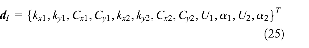
where subscripts 1 and 2 respectively denote the left (#15) and right (#16) bearing. The response components u_c, v_s, u_s, v_c at two bearings reflect the severity of rotor unbalance and are selected as the features in this approach. The feature vector is hence defined as

$$\mathit{f}=\{u_{c1},u_{s1},v_{c1},v_{s1},u_{c2},u_{s2},v_{c2},v_{s2}{\}}^T$$

(23)

In the following, $\mathit{f}\mathrm{and}\stackrel{-}{f}$ denote the theoretical (calculated) and measured (real) feature vector, respectively. The residual is defined as the sum of absolute errors of the eight feature variables, that is,

$$e={\sum }_{i=1}^8|f_i-{\stackrel{-}{f}}_i|$$

(24)

A smaller residual implies less difference in response between model calculations and real measurements under a specific unbalance configuration. Therefore, searching for the global minimum of residual will yield the most appropriate unbalance estimation in the specified domain. The optimization is two-phase and the parameters to be identified in phases I and II are respectively written as

$${\mathit{d}}_I=\{k_{x1},k_{y1},C_{x1},C_{y1},k_{x2},k_{y2},C_{x2},C_{y2},U_1,{\alpha }_1,U_2,{\alpha }_2{\}}^T$$

(25)

$${\mathit{d}}_{\mathrm{II}}=\{U_1,{\alpha }_1,U_2,{\alpha }_2{\}}^T$$

(26)

The parameters to be identified in phase I include the bearing constants and the initial unbalances, (U_1,α ₁ ) and (U_2,α ₂ ) quantified at the two bearing planes. It is known that balancing a flexible or quasi-flexible rotor requires multi-plane calculations (at least two planes). As shown in Figure 2(a), the first and third disk planes are adopted as the balancing planes at every overhaul. A rotor’s total unbalance is usually divided into two parts, the so-called static and dynamic unbalance. These two terms respectively denote the offset of gravity center and the angle of principal rotary inertia axis away off the rotation axis. The static and dynamic unbalances can be combined and configured into unbalances at any two arbitrary planes and vice versa. In the present identification process, the unbalances of two bearing planes instead of the two disk planes are selected for identification. The reason is that the unbalance phases at two bearing planes are much easier to be localized from the measured response with the aid of model calculations. It has been found that the specification of phase range for optimal solution search is crucial. The searched results were sometimes trapped in the local minimum rather than the global one if the unbalance phases were unenclosed.

The way of enclosing the unbalance phase is described below for the left bearing as an example. The response at the left bearing is due to left and right unbalance excitations. It has been numerically solved that the cross receptance, ³⁷ that is, the left harmonic response due to right harmonic excitation and vice versa, has a magnitude order about one-tenth of the direct receptance. In addition, no cross stiffness and damping coefficients are included in the bearing properties so that u and v can be treated as uncoupled. That means that the x-direction response of the left bearing can be approximated as just due to the left unbalance force. According to equations (10) and (11), the unbalance forces at the left bearing, in horizontal and vertical directions, are

$$F_{x1}=U_1{\mathrm{\Omega }}^2\cos (\mathrm{\Omega }t+{\alpha }_1)\delta (z-z_1),$$

(27)

$$F_{y1}=U_1{\mathrm{\Omega }}^2\sin (\mathrm{\Omega }t+{\alpha }_1)\delta (z-z_1)$$

(28)

where the initial unbalance amount and angle (U_1,α ₁ ) are unknowns. Meanwhile, the measured response in x and y directions, according to equations (17) and (18), can be expressed as

$$u(z_1,t)=A_{x1}\cos (\mathrm{\Omega }t-{\varphi }_{x1})$$

(29)

$$v(z_1,t)=A_{y1}\cos (\mathrm{\Omega }t-{\varphi }_{y1})$$

(30)

where A’s and ϕ’s are the measured response amplitudes and phases fitted from the acquired data. The x response (29) would have a phase lag, θ _x1 , relative to the excitation because of the existing damping and this phase lag can be assumed as

$${\theta }_{x1}={\varphi }_{x1}+{\alpha }_1$$

(31)

Similarly, the phase lag in y response can also be obtained and denoted as well,

$${\theta }_{y1}={\varphi }_{y1}+{\alpha }_1-\pi /2$$

(32)

Combining (31) and (32), the unbalance phase at the left bearing plane, based on the measured response, can be enclosed inside the following parentheses

$${\alpha }_1\in ({\theta }_{x1}-{\varphi }_{x1},{\theta }_{y1}-{\varphi }_{y1}+\pi /2)=({\alpha }_1^L,{\alpha }_1^H)$$

(33)

Nonetheless, the phase lags, θ_x1, θ _y1 , in equation (33) due to damping are still unknown. Since the system damping is relatively low, it is feasible to assume a large enough phase lag so that the unbalance angle will be bounded in a suitable range to facilitate solution search. This has been proven effective in saving computational time and assuring global minimum. An interesting case of equal phase lag in x and y response (θ _x1  = θ_y1) and measured phase ϕ _y1 being exactly 90° lag of ϕ_x1 will yield an exact single value instead of a region, that is, precise location of unbalance phase.

Parameter identification

Parameter identification/estimation is the most crucial step in a model-based fault diagnosis approach. Some model parameters derived from physical theories can closely represent the real system such as shaft mass and stiffness. Some others are yet not so certain even if they can be obtained from theoretical calculations. These include bearing stiffness and damping. To assure the derived model well represent the real machine, applying measured data to tune the model parameters in an optimal sense is a necessary and important step. This process can be categorized as parameter identification or model-updating.

Parameter identification process in the present approach is divided into two phases, both via optimization schemes. In phase I, eight bearing parameters plus four initial unbalance variables right after an overhaul are evaluated. As the bearing parameters are determined, the progression of unbalances at two bearing planes is evaluated in Phase II. The reason of not using the residual unbalances at overhaul in phase I is that the original unbalances, obtained under the class of 2G, ³⁸ are mostly related to rigid unbalance. The present rotor’s response, however, comprises the shaft’s flexible deformation. Thus, the initial unbalances, characterized by two components at the left and right bearing planes, are treated as undetermined parameters in the beginning of identification process, so are the bearing parameters.

Optimization algorithms

In phase I identification, the first three sets of data, one set per day, under steady-state condition right after an overhaul are selected. Five different optimization algorithms were tested in both phases, which are generic algorithm (GA), ³⁹ grey wolf optimizer (GWO), ⁴⁰ grey wolf optimizer with cuckoo search (GWOCS), ⁴¹ whale optimization algorithm (WOA), ⁴² and Particle Swam Optimization (PSO) algorithm.^43–45 The results yielded by these five algorithms are slightly different from one another and at last, the PSO algorithm provided by MatLab toolbox is selected for solution search because it has the advantages of less parameters tuning, easy constraint, robust and fast for objective optimization.

The optimization problem in phase I can be summarized as the following,

$$\{\begin{array}{c}mine={\sum }_{i=1}^8|f_i({\mathit{d}}_I)-{\stackrel{-}{f}}_i({\mathit{d}}_I)|\hfill \\ \multicolumn{1}{c}{\mathrm{subject}\mathrm{to}}\\ \multicolumn{1}{c}{U_1,U_2\le 1000\mathrm{g}·\mathrm{mm}}\\ \multicolumn{1}{c}{150\le k_i\le 350\mathrm{MN}/\mathrm{m}}\\ \multicolumn{1}{c}{\begin{array}{c}2\le C_i\le 200\mathrm{kN}·\mathrm{s}/\mathrm{m}\hfill \\ \multicolumn{1}{c}{{\alpha }_1\in [{\alpha }_1^L,{\alpha }_1^R]}\\ \multicolumn{1}{c}{{\alpha }_2\in [{\alpha }_2^L,{\alpha }_2^R]}\end{array}}\end{array}$$

(34)

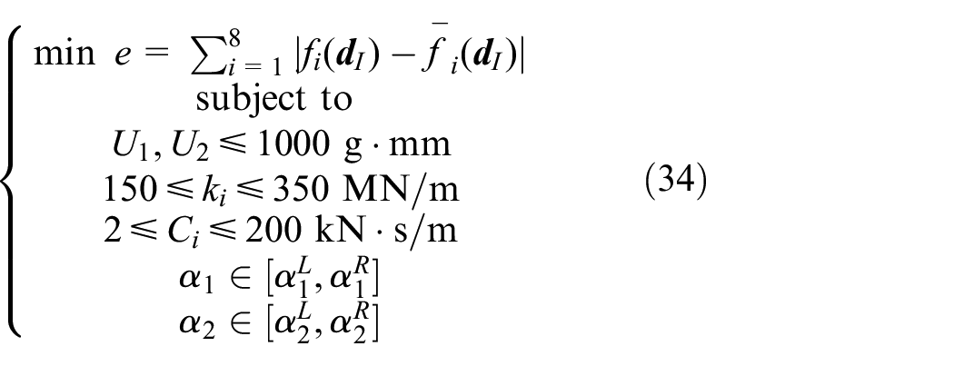
The searching ranges for bearing stiffness and damping coefficients are determined based on theoretical calculations and references of hydrostatic bearings.^31,46 The 12 parameters obtained in phase I for the three sets of data are listed in Table 1. The residuals, equation (24), of these three sets are respectively 2.73, 2.21, and 2.70 μm. As seen, the second set yielded the smallest error and is chosen as the model parameters to proceed to phase II.

Table 1.

Estimated parameters using the first three sets of steady-state operational data.

Bearing parameters C (kNs m−1), k (MN m−1)								Unbalance U (g mm) and α (degree)
Cx1	Cx2	Cy1	Cy2	kx1	kx2	ky1	ky2	U1	α1	U2	α2
100.0	200.0	48.0	2.0	347.7	153.3	287.8	311.0	668.	38.1	306.	−96.9
160.3	182.2	55.1	2.0	335.5	129.2	328.2	288.0	747.	38.1	279.	−96.9
142.3	200.0	36.6	2.0	347.8	130.2	321.2	305.7	746	33.6	344.	−85.6

In the process of phase II, one set of data per day is retrieved and used to continuously estimate the progression of unbalances, where the optimization problem can be described as

$$\{\begin{array}{c}mine={\sum }_{i=1}^8|f_i({\mathit{d}}_{\mathrm{II}})-{\stackrel{-}{f}}_i({\mathit{d}}_{\mathrm{II}})|\hfill \\ \multicolumn{1}{c}{\mathrm{subject}\mathrm{to}}\\ \multicolumn{1}{c}{U_1\le 1.2U_1(\mathrm{latest}\mathrm{one})}\\ \multicolumn{1}{c}{\begin{array}{c}{U}_2\le 1.2U_2(\mathrm{latest}\mathrm{one})\hfill \\ \multicolumn{1}{c}{\begin{array}{c}{\alpha }_1\in [{\alpha }_1^L,{\alpha }_1^R]\hfill \\ \multicolumn{1}{c}{{\alpha }_2\in [{\alpha }_2^L,{\alpha }_2^R]}\end{array}}\end{array}}\end{array}$$

(35)

The constraint of unbalance quantities U₁ and U₂ less than 20% increment of the latest ones is deliberately set up for computational efficiency, because unbalance deterioration hardly exceeds 20% over 1-day operation unless a sudden broken down occurs. and the identified results confirmed this assumption.

Model validation

The rotor’s model has been validated with FEM results. Now, the rotor-bearing combination with the identified bearing parameters obtained in Phase I is examined prior to unbalance evaluation in phase II. The manufacturer provides very little information except the first two critical speeds being near 5000 and 19,900 rpm. Since the rotor is of trans-critical operation the rotor’s transient response during shutdown will provide us the information of the actual first critical speed. By inspecting the machine’s shutdown transient, it is found the first critical speed occurs near 4655 rpm (77.6 Hz). Table 2 lists the calculated critical speeds using the sets of parameters given in Table 1. The results show that all the calculated first critical speeds are very close to 4655 rpm with errors less than 1.5%. This consistency enhances the appropriateness of identified parameters in Phase I. As to the second critical speed, since there is no operational data for validation, the calculation can only be compared against the manufacturer’s data and the difference falls within the range of $\pm 6\%$ . From Table 2, it is also seen that the critical speeds in x and y direction are slightly different due to asymmetry of bearing parameters. The critical speed in y direction appears slightly higher than that in x, and it is usually true because the rotor weight squeezes the oil-film more in y direction and increases the bearing stiffness. The critical speeds at operational speed are also shown in Table 2. As expected, critical speeds shift about 1% down because rotation softens the stiffness matrix as seen in equation (3).

Table 2.

Calculated critical speeds (rpm) of the turbine-bearing system.

Critical speeds (rpm)	Set 1		Set 2		Set 3
	Ωcr		Ωcr		Ωcr
at Ω = 0	x	y	x	y	x	y
1st	4593	4628	4568	4633	4583	4637
2nd	18,690	21,149	18,746	22,797	18,741	21,022
at Ω = 11,000	x	y	x	y	x	y
1st	4511	4578	4497	4574	4512	4577
2nd	18,106	20,703	18,198	21,182	18,201	21,053

Unbalance monitoring and prognosis

A rotor’s balance would deteriorate with time and loading under long-term operation. This deterioration is reflected through the increase of vibration response. Conventional monitoring approach can detect the difference of vibration at each sensing point but is unable to provide quantitative contrast between vibration increment and unbalance deterioration. The aim of this step is to integrate all sensors’ data and evaluate the unbalance deterioration based on the derived approach.

Unbalance evaluation and monitoring

The operational data used to validate the developed algorithm were acquired over a time interval of 16 months provided by a local plastic company. A pilot run was first launched in which one data set per 10 days is adopted in running phase II. Figure 4 illustrates the evaluated unbalances (amounts and phases) evolve with time at two bearing planes, where the unit of ordinate is $g·\mathrm{mm}$ for unbalance amount and that of abscissa is the running days (x10). The results show that both unbalance phases vary gradually within a small range, which is a positive indication of the approach’s convergence because the unbalance phase hardly change abruptly unless a sudden fault occurs. The phase fluctuation is anticipated and can be attributed to the torsional vibration of shaft. The shaft’s torsional vibration, which has not been considered, will affect key phasor timing and cause the fluctuation of sensing reference.

Figure 4.

The evaluated unbalances varying with time at two bearing planes.

Figure 4 also shows, over a 16-month period of time, U₁ maintains about the same level while U₂ and α₂ experience a sudden change around the 130th day. After consulting with company’s engineers, it is noticed the factory disclosed a labyrinth-ring broken event inside turbine during that specific time interval. After repair, the vibration at bearing #16 significantly increases for unknown causes. Meanwhile, the phase α₂ drifts about 40°. This outcome is not surprising at all because labyrinth-ring replacement will certainly change the rotor’s balance status, both in amount and phase angle. The present approach truly reflects this event by showing the sudden unbalance change.

Figure 5 illustrates the unbalance deterioration in terms of commonly described in rotor industry the static and dynamic unbalance, which are directly configured from the unbalances of two bearing planes. To comprehend the unbalance deterioration, two ordinates are labeled on the magnitude plots, one for the absolute amounts (left) in a unit of ( $g·\mathrm{mm}$ )and the other for the ratios (right) compared to the initial unbalance. To the authors’ opinion, the ratios provide more clear indication than the absolute amounts because the rotor response contains the shaft’s flexible deflection, which was not included in the balancing at a low speed. The blue curves shown in the plots are the smoothened ones. The evaluation indicates that static unbalance worsens at a ratio of 2 and the dynamic one is about 1.2 times of the initial during 16-month operation. That means the mass center eccentricity is more seriously than the orientation changes of rotary inertia’s principal axis. The results were confirmed by the collaborated company at the next overhaul wherein the static unbalance degradation was found much worse than that of dynamic one. The identified deterioration trend is also consistent with the real situations found at overhaul. This comparison partially proves the feasibility of this approach as implemented in the in-situ rotor monitoring system.

Figure 5.

The evaluated static and dynamic unbalance of the turbine-bearing system.

The robustness of the derived approach is another issue of concern. To answer this concern, the static and dynamic unbalance curves are solved for by five different optimization algorithms as previously depicted. The five algorithms yield very consistent results, as shown in Figure 6, and this result proves the robustness of the derived approach. The variations of resultant residuals, equation (24), through the whole time period obtained by these five algorithms are also compared in Figure 7(a). It is seen that these curves surprisingly coincide with one another. In summary, the residual is below 3.5 μm before the labyrinth rings replacement, but it increases to around 5.5 μm in average after the major repair. The coincidence of residual curves infers that all of these algorithms are equally accurate. Nonetheless, PSO algorithm provided by MatLab toolbox was chosen after comparing the computational efficiency of these five algorithms. Figure 7(b) shows the differences between the curves of feature-sum (in absolute value) and the residual by PSO. It is observed that the residual curve closely resembles that of feature-sum.

Figure 6.

Static and dynamic unbalance obtained via five algorithms.

Figure 7.

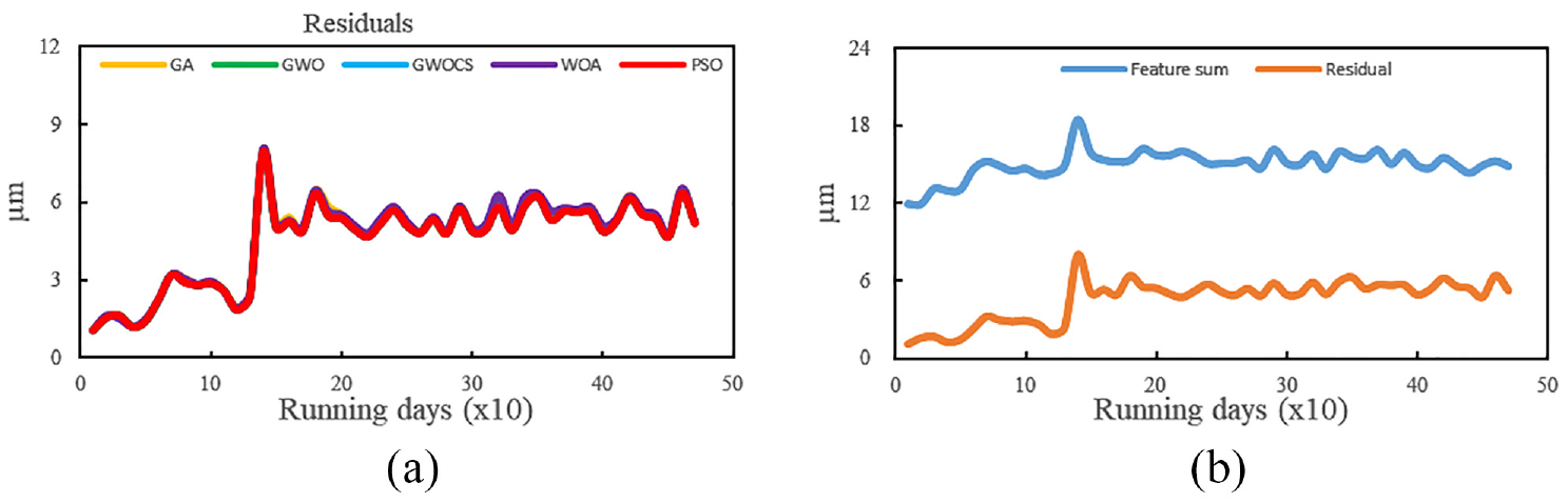
(a) The resultant residuals of five different algorithms and (b) the difference between feature-sum and residual by PSO.

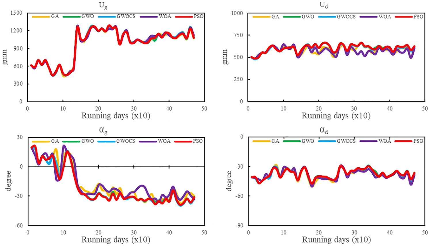
Figure 8 illustrates the developing unbalances on a daily base, that is, one dataset per day, during the 16-month operation. The results are consistent with those presented in Figure 6 but have more fluctuations in both static and dynamic unbalance curves. The sudden change of phase angle α _g around 130th day truly reflects the fact of labyrinth rings change event. This result proves the effectiveness of model. After the major repair, the static and dynamic unbalance phase angles approaching constant values also imply the stability and convergence of the searching algorithm.

Figure 8.

Developing static and dynamic unbalance monitoring on a daily base.

Unbalance prognosis/forecasting

Finally, the unbalance prognosis/forecasting capability of the approach is discussed. The forecasting scheme is using a certain time period of identified unbalances and extrapolating the curve for the forthcoming future prediction. The present model adopts simple autoregressive (AR) model^47,48 as a demonstration, that is, using a linear combination of past values of unbalance indexes (variables) to forecast the future unbalance indexes. The term of AR indicates that the output variable depends linearly on its own previous values. Thus, the AR of order $p$ can be formulated as:

$$y_t={\theta }_1{y}_{t-1}+{\theta }_2{y}_{t-2}+\dots +{\theta }_p{y}_{t-p}+{\epsilon }_t$$

(36)

where ${\epsilon }_t$ is white noise and following an $\mathrm{N}(0,{\sigma }^2)$ $·{\sigma }^2$ and ${\theta }_1,..{\theta }_p$ are unknown model parameters. These parameters can be estimated on the basis of observation on y using maximum likelihood.^48,49

The demonstrated example shown in Figure 9 is using the most recent 3 months’ unbalance data to forecast the forthcoming month using the AR model of order four. The forecast function continuously collected the past 3 months’ data then launched the prediction of the next month’s unbalances. The curves of real happening (in blue) and forecasted (in orange), progressive with time, are superimposed in Figure 9 for comparison. These two curves well match each other except there is a time delay in the region of unusual sudden rise. In spite of that, the forecasted unbalance closely resembles the developed one. The forecasted section (1 month in advance) can work as a prognostic function for rotor unbalance and provides valuable information for CBM strategy making. The capability of unbalance prognosis in the derived algorithm, to the authors’ understandings, is the first one demonstrated in the literature. Figure 9 only demonstrated a feasible way of unbalance prognosis using simple regression algorithm as AR model. It is conceivable that longer past historical data and more sophisticated regression model may lead to more reliable and longer forecasting.

Figure 9.

Comparison of developed and forecasted unbalance with time.

Conclusions

A novel model-based approach for real-time, online, unbalance monitoring and prognosis of rotor-bearing system is developed in the present research. The rotor alone was first validated with an FEM result and the rotor-bearing model was next validated with the machine’s operational data. Both results show excellent consistency. Through the investigation, the authors have arrived at the following conclusions in the aspects of methodology and analytical results.

Regarding the methodology: (1) Two-phase parameter identification works well for the rotor-bearing identification, in which the initial unbalances and bearing parameters are simultaneously identified in Phase I and the progression of unbalances is evaluated in Phase II. (2) The robustness of method is proven via five different optimization algorithms. As to the analytical results, over 16 months’ data analyses reveal that: (1) The deterioration ratios of static and dynamic unbalance with respect to their initial counterparts are, respectively, 2.0 and 1.2, and the trends consist with the factory’s balancing data at two consecutive overhauls. (2) Using the past 3-month data to forecast the forthcoming month is a feasible way for unbalance prognosis. (3) Unbalance curves of the real happening and predicted one show excellent consistency. Discrepancy between them, however, happens at the place where abrupt change of unbalance occurs due to fault event, like the case of ring repair, which suddenly changes the rotor’s balance status. The demonstrated results have proven the effectiveness and robustness of the developed approach for online, real-time monitoring and prognosis of rotor’s unbalance. Thus, it is implanted into a local industrial rotor system as a part of CBM maintenance system.