
Abstract
This article presents a design procedure for structural health monitoring systems based on bulk wave ultrasonic sensors for structures fabricated from polycrystalline materials. When designing a monitoring system, maximum coverage per transducer is a general requirement in order for the system to be economic. For coarse-grained polycrystalline materials, monitoring is often made challenging by low signal-to-noise ratios caused by grain scattering. Therefore, when designing a monitoring system for these materials, in addition to the economic requirement, it needs to be ensured that an adequate signal-to-noise ratio can be obtained throughout the monitoring volume. This typically introduces a trade-off between volume coverage per transducer and sensitivity that must be investigated. In this article, this trade-off is studied and a methodology using signal-to-noise maps is presented to design the system, that is, choose the optimal transducer parameters and placement. First, a combined analytical and numerical approach is used to generate a signal-to-noise map. Then, the influence of various factors on signal-to-noise ratio is investigated. Finally, two representative examples, with different criteria, are given to illustrate the methodology. In one example, the full surface area of the testpiece is covered with transducers and the optimum gives the deepest coverage. The other one aims to achieve the minimum fractional surface area that has to be covered with transducers to monitor a narrow depth range far from the surface, which has a potential application in weld monitoring. Results show that the optimum is likely to be at much lower frequency than typically used in inspection, as tracking signals with time gives sensitivity gains. Experiments were carried out to illustrate that higher volume coverage can be obtained at lower frequencies.
Keywords
Introduction
Grain scattering, due to the acoustic impedance contrast caused by different alignments of principal axes of the grains/colonies, 1 often results in a low signal-to-noise ratio (SNR) in ultrasonic inspection of coarse-grained polycrystalline materials. In order to enhance the SNR, many techniques have been researched, including inspection techniques, aiming at achieving good SNRs in raw signals in the procedure of inspection, and processing techniques, which enhance the SNR by processing raw signals with low SNRs. Multizone2–4 is a widely used inspection technique, which uses multiple focused transducers focusing at different depths to scan a sample. This enables most of the material to be covered in the focal zone, so that good SNRs can be achieved throughout the sample. Split spectrum processing (SSP)5–7 and wavelet transform de-noising methods8–10 are widely researched signal processing techniques, which suppress the grain noise in raw signals to enhance the SNR but show limited improvement.
A structural health monitoring (SHM) approach in which a baseline reading is subtracted from a current reading can remove temporally coherent signals, provided adequate compensation for environmental changes is applied.11,12 Therefore, if it is assumed that the ultrasonic properties of the grains are unaffected by ageing, 13 grain noise is coherent and this baseline subtraction technique is feasible.
Generally, there are two means to conduct SHM, repeat scanning 14 and permanently installed monitoring.15,16 To compare a current inspection result to a past test, repeat scanning requires the scans to be precisely registered so that the signals from the same point can be compared. A recent study showed that with repeat scanning, baseline subtraction, along with compensation methods for environmental changes, gives a relatively modest improvement in SNR. 14 Permanently installed monitoring is free of the registration problem as transducers are permanently installed at fixed positions. However, fixed transducers make scanning impractical. Therefore, a set of fixed transducers needs to cover the whole required inspection volume and in order for the system to be economic, it is desirable for each transducer to cover as large a volume as possible; this typically introduces a trade-off between volume coverage per transducer and sensitivity that must be investigated. This is studied in this article.
Focused transducers are often used to improve SNRs, for example, when using the multizone scanning technique. However, as they can only improve the SNR near the fixed focal zones, leaving low SNRs outside of the focal areas, they are less desirable than unfocused ones in a permanently installed monitoring system, where relatively uniform sensitivity is required through the whole volume of the testpiece. Therefore, unfocused transducers are considered in this article.
An unfocused transducer with a large beam spread is desirable for coverage, but low amplitude at the edge of the beam causes poor SNRs. To investigate the trade-off between volume coverage per transducer and sensitivity, good understanding of different determining factors is required. Many studies have been carried out to understand the behaviour of defect reflection,17–19 grain noise20–22 and scattering-induced attenuation,23–26 which affect the sensitivity of the transducer, as a function of frequency. The beam spread of a transducer is determined by the transducer diameter-to-wavelength ratio. 27 Therefore, using transducers with different frequency, diameter and placement for the monitoring system significantly influences the volume coverage and detection sensitivity.
The goal of this article is to design an optimised monitoring system. This will be defined as a system requiring minimum number of transducers (and hence lowest cost) to cover a given volume of structure at a given required minimum SNR for a given type and size of defect. An analytical and numerical approach is proposed to produce SNR maps generated by different transducers, which show their volume coverage and sensitivity. Then, according to a given criterion and requirements, the optimal transducer parameters and placement can be found.
This article begins by introducing the optimisation problem to be solved, including the criteria and requirements often imposed. Then, an approach to produce an SNR map is presented. The signals from a flat-bottom hole, representing a calibration defect, at one position are computed using the Thompson–Gray model. 19 The grain noise is predicted using the theoretical solution given by Liu et al., 21 which is also based on the Thompson–Gray model. The scattering-induced attenuation is obtained using POGO, a highly efficient GPU-based solver, 28 enabling overall SNR maps to be produced. The article then investigates how various factors affect the SNR value and its distribution. Two possible optimisation criteria are given and two representative examples showing how to find the optimum transducer parameters and placement under each criterion are discussed, with experiments illustrating a key conclusion.
Optimisation problem
As discussed above, the goal of this article is to design an optimal system to monitor a given volume of structure at a given required minimum SNR for a given type and size of defect with the lowest cost. This leads to an optimisation problem which usually gives a criterion related to the cost of the system as the target and some requirements related to the SNR value and distribution in the given volume to be monitored. In this section, possible criteria and requirements of the optimisation problem are given and they will be used later in section ‘Case studies’.
As shown in Figure 1, a monitoring system designed to cover a given region of structure is considered. It comprises multiple identical transducers of diameter, D, and uniform spacing, S. As discussed in section ‘Introduction’, unfocused transducers are used, therefore, due to beam spread, each transducer can cover a conical volume. In this example, the system is to monitor the whole volume of the structure beyond a depth, d, so each transducer needs to monitor a cylindrical volume which is referred to as the inspection cylinder here.
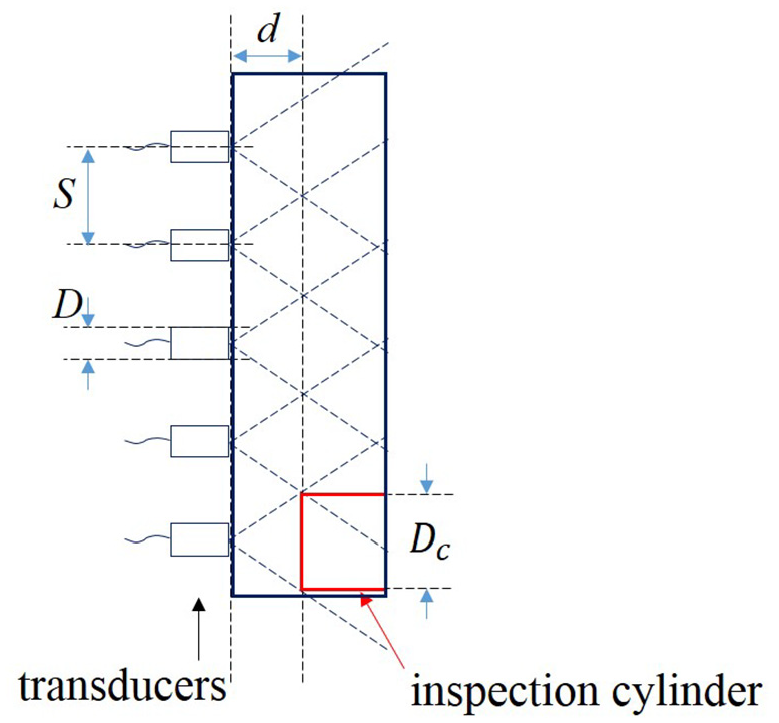
Schematic diagram of permanently installed monitoring system.
In the limit, if the minimum depth from which the inspection volume starts is small, then the cylinder becomes narrow and in the limit approaches the diameter of the transducer, implying that the full surface area of the structure is covered with transducers, so the spacing, S, becomes equal to the transducer diameter, D. Therefore, the fractional surface area covered with transducers, which is defined as the ratio of the squared transducer diameter to the squared inspection cylinder diameter (
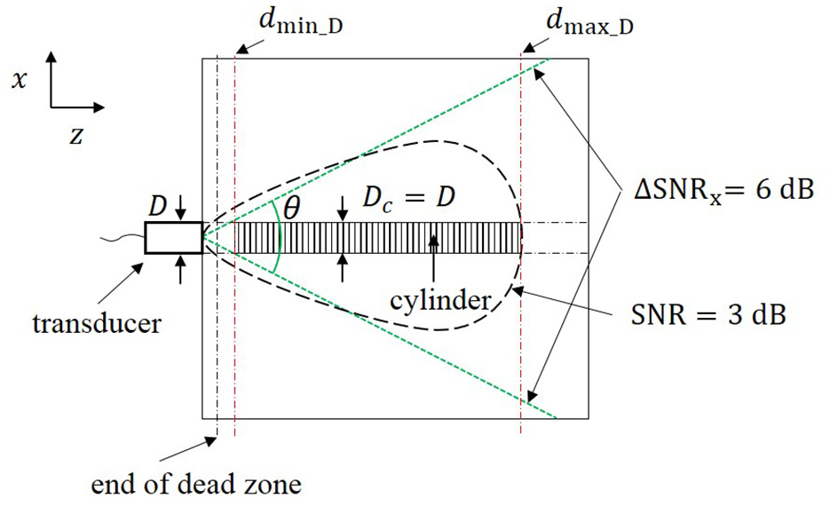
As the minimum depth that must be covered increases, a relatively large spacing can be used, at the cost of losing detection ability at the shallow part of the structure. An example of this is the need to monitor a weld for defects on the fusion face as shown schematically in Figure 2. Assuming that the transducers are lined up parallel to the weld, the transmit–receive distances are similar over the whole fusion face, so it is equivalent to monitoring over a narrow depth range relatively far away from the transducer. As indicated in Figure 2, the practical weld application requires an angle beam with a skip off the back wall, but in the simplified examples considered in this article, coverage over a narrow range of depths at normal incidence is investigated to show the principles of the optimisation. In this case, a small transducer being able to cover a large area relative to the transducer surface in the given depth range is desirable. Therefore, the criterion of the optimisation problem is that the optimal transducer gives the smallest fractional surface area that has to be covered with transducers to monitor the required depth range over the whole testpiece.
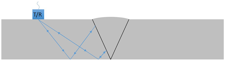
Weld monitoring geometry.
To obtain satisfactory coverage and detection sensitivity within the required inspection cylinder and also for practical reasons, the optimisation problem often requires
A minimum SNR value in the inspection cylinder;
A maximum radial variation of SNR in the inspection cylinder to ensure a given sized defect at any radial location at a given depth gives a similar reflection amplitude, which is required for defect sizing; since the noise is constant in the radial direction, this condition is equivalent to a requirement on the maximum variation in signal across the inspection cylinder at a given depth. There is no equivalent requirement for constant amplitude with depth, as signals from different depths appear at different times and so can be compensated by standard distance–amplitude correction (DAC); 29
A minimum transducer diameter to ensure that it is practical to construct and deploy with the appropriate cables;
A minimum transducer diameter-to-wavelength ratio to provide efficient generation of a normal incidence longitudinal wave; 30
The inspection cylinder to be beyond the dead zone (
The inspection cylinder diameter to be greater than or equal to the transducer diameter to avoid the need to overlap transducers to obtain full coverage.
Schematic diagrams of SNR maps under the two criteria (referred to as Criterion 1 and 2, respectively) are shown in Figure 3, where the minimum SNR is set to be 3 dB and the maximum radial variation of SNR is set to be 6 dB as example requirements. In this article, a flat-bottom hole is used as a calibration defect, as normal incidence is considered. However, the same methodology can be used for different types and orientations of defects.
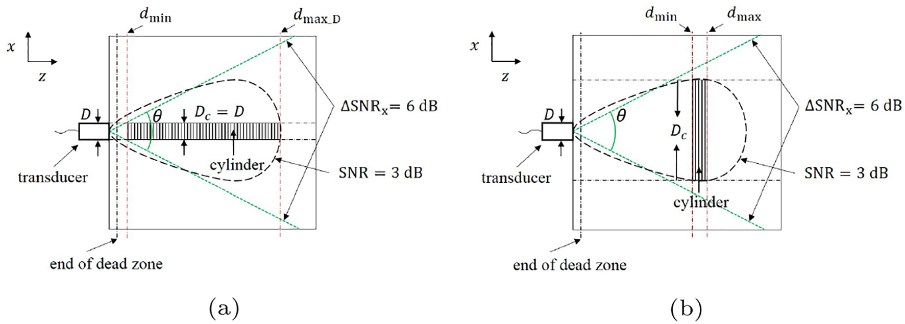
Schematic diagrams of SNR maps under (a) Criterion 1 and (b) Criterion 2. D and
SNR map generation
To solve the optimisation problem, it is essential to have a good knowledge of the SNR map produced by a single transducer, which, in this article, is a bonded piezoelectric transducer (PZT). Each point in the SNR map shows the ratio of the peak amplitude of the reflection from a defect at that position to the root mean square (RMS) grain noise level received at the same time. A theoretical solution of SNR has been developed by Margetan et al., 31 where the SNR is independent of attenuation, as it is assumed that the effective attenuation coefficients are identical for the signal and backscattering noise. However, it has been found that the scattering-induced attenuation has a more significant influence on the coherent waves than the grain noise, which means that the SNR is dependent on the attenuation.31–33 Furthermore, it has been pointed out that it is reasonable to ignore the influence of the scattering-induced attenuation on the grain noise. 21 Thus, in the procedure of SNR map generation in this article, the attenuation, deduced using the coherent waves, is ignored in the noise calculation but considered in the signal prediction, which is different from the model given by Margetan et al. 31
In this section, a combined analytical and numerical approach to generate a three-dimensional (3D) SNR map is introduced. First, the particle velocity field in a homogeneous isotropic material, of which the material properties are the Voigt averages of the polycrystalline material to be investigated, is predicted using ABAQUS. Then, based on the Thompson–Gray model, the reflection from a defect and the RMS grain noise are calculated theoretically using the particle velocity field where no scattering-induced attenuation is considered. Finally, by adding an attenuation term, which is obtained with the polycrystalline material using POGO, an overall SNR map is produced.
Particle velocity field and Gaussian beam fitting
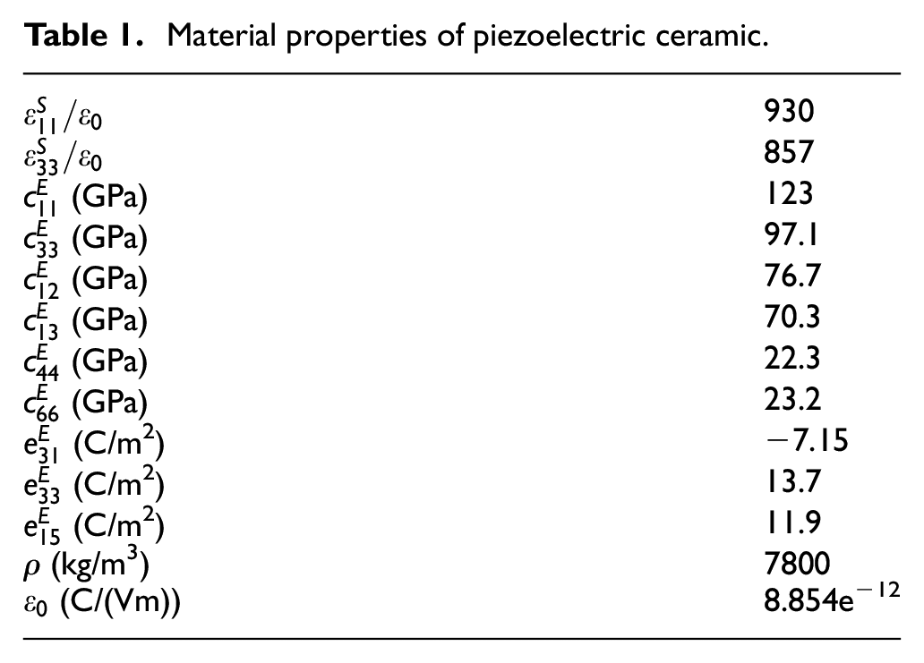
To obtain an SNR map, it is essential to know the particle velocity field generated by the transducer, which determines the received defect reflection and grain noise. The velocity field is predicted using implicit dynamic analysis in the commercial finite element (FE) software ABAQUS, in which, unlike the current version of POGO, piezoelectric elements are enabled. A three-cycle toneburst voltage with a peak amplitude of 1 V is applied between the opposite faces of the PZT element. The initial aim was to investigate the effect of excitation frequency on SNR. The amplitude and beam pattern generated by a piezoelectric disc is a significant function of the disc thickness; this was fixed at 4 mm in the initial study in order to give satisfactory response across the frequency range of interest that included frequencies as low as 100 kHz where the response from thinner discs is very low. A bond line with a thickness of 0.05 mm is modelled between the PZT and the testpiece. The material of the bond line is epoxy, of which Young’s modulus, density and Poisson’s ratio are 2.8 GPa, 1200 kg/m3 and 0.345, respectively. The material properties of the PZT are given in Table 1.
Material properties of piezoelectric ceramic.
Because the transducer is axisymmetric, the velocity field produced by it can be predicted with the two-dimensional (2D) axisymmetric model shown in Figure 4, where the blue long-dash line at the top edge shows the axis of symmetry and the PZT is bonded to the left edge of the testpiece. The receivers are uniformly distributed in the model to give the displacement signals, and by taking the derivative with respect to time, the velocity signals can be obtained. The velocity field is then generated by taking the peak amplitudes of the velocity signals.
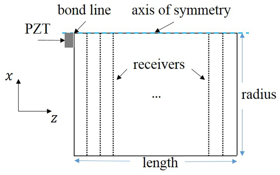
Schematic diagram of an ABAQUS 2D axisymmetric model with uniformly distributed point receivers used to predict velocity field.
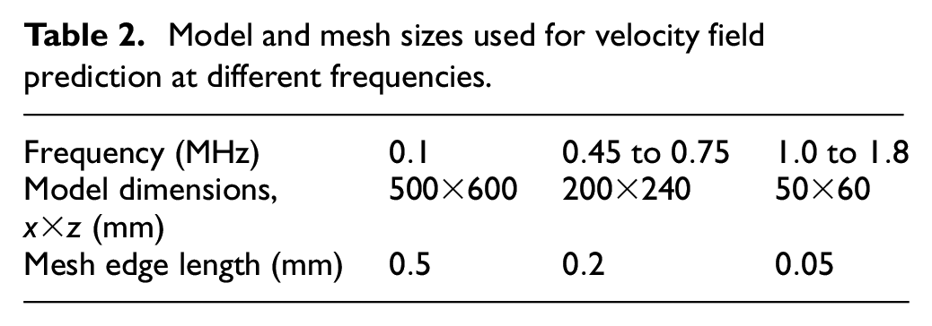
Relatively large models are used to minimise the boundary effect on the velocity field; as the insonified area is larger with a lower frequency, larger models are used in the lower frequency cases. Details of the model and mesh sizes (structured quadrilateral element) used for velocity field prediction are given in Table 2.
Model and mesh sizes used for velocity field prediction at different frequencies.
A 3D velocity field with uniformly distributed data points can then be generated using a 3D Gaussian beam model which gives the best fit to the 2D field; this is easier to implement than interpolating the FE results for all the points on interest, and the model also allows extrapolation. In the following calculation of defect reflection and RMS grain noise level, the fitted Gaussian beam model will be used to describe the particle velocity field.
Defect reflection prediction and noise calculation
In this section, the peak amplitude of the defect reflection and the RMS grain noise level received at the same time as the defect reflection peak arrives are calculated; these are used to generate the SNR map later.
A flat-bottom hole is used as a calibration defect and the reflection from it is predicted using the Thompson–Gray model 19
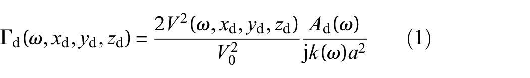
where
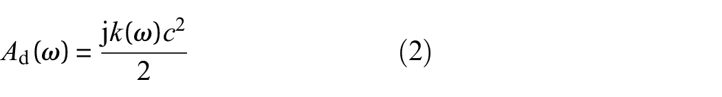
where c is the radius of the defect.
Assuming the transducer is excited by a toneburst

the peak amplitude of

In the time domain, if all the constants and functions which are slowly varying with

where
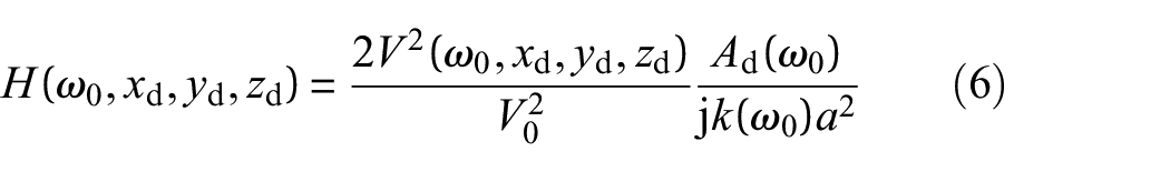
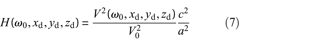
Comparing equations (5) and (3), it can be seen that the reflection from a defect is a time-shifted copy of the excitation signal modified by the factor of H. If it is assumed that the envelope function
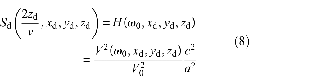
Based on the independent scatterer model, 22 the RMS grain noise level received at time t is calculated using the theoretical solution given by Liu et al. 21
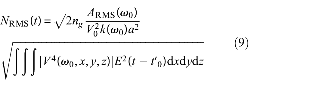
where
According to equation (9), the RMS grain noise level received at time
Equations (8) and (10) are used later for SNR calculation.
Scattering-induced attenuation
So far, attenuation has not been accounted for in the calculation. In this study, only the attenuation induced by scattering, which has a significant impact on coherent signals, is considered.
A 3D grain model, shown in Figure 5, is used to predict the coherent attenuation coefficient. The model with dimensions of
Schematic diagram of the 3D grained model used for attenuation prediction.
Cubic single-crystal symmetry is considered for the grains in this study. The cubic material whose Voigt averages are used in the velocity field and defect reflection calculations is assigned to the model, with different orientations to different grains. Symmetry boundary conditions are used on the model surfaces parallel to the z-axis, making the model equivalent to being infinitely wide with repeating grain structures. All the nodes on one of the model surfaces in the
The attenuation coefficient is then used to estimate an attenuated reflection amplitude received by a finite transducer. If it is assumed that the modelled transducer is centred at the origin, the attenuated reflection amplitude from a defect at
SNR map generation
Based on the previous three sections, with a defect located at
An SNR map can then be generated for a certain volume, with each point in the map showing an SNR value assuming that there is a flat-bottom hole located at that location. It should be noted that due to the assumptions of the theoretical solution of the defect reflection, the map generated with the proposed procedure is a first estimate and is liable to be less accurate when the defect size-to-wavelength ratio increases beyond unity. The information of the SNR value and its distribution produced by a bonded PZT element can then be obtained with this SNR map, from which the optimal transducer can be found. Before two examples are introduced to show how to solve the optimisation problem using SNR maps, in the next section, the effects of different determining factors of SNR are discussed, which is essential to obtain a good understanding of the result of the optimisation problem.
Factors influencing the SNR
The SNR is determined by a combination of factors, including defect characteristics, material properties, excitation, and transducer parameters. More specifically, defect type and size strongly affect the signal amplitude; grain size and anisotropy factor significantly influence the noise and attenuation; excitation type and duration determine the grains and their weights contributing to the noise at a given time instant; transducer frequency and diameter both have a substantial impact on the signal and noise, and transducer frequency also affects the attenuation. As the SNR is a function of so many variables, it is difficult to understand the result of the optimisation problem without a good understanding of how these factors affect the SNR.
In this section, taking a flat-bottom hole as a calibration defect, the SNR dependence at different locations on the various factors (except the defect type) is investigated.
Effects of excitation parameters
In this article, it is assumed that the inspection frequency is centred at the resonance frequency of the transducer, therefore, it is considered as a transducer parameter to be optimised and the influence of the transducer frequency on SNR will be investigated later. Here, the influence of the shape and duration of the excitation is discussed. The noise can be regarded as a weighted sum of the reflections from grains,
31
of which the number and weights are determined by the envelope function of the excitation (
Effects of grain size
Compared to the excitation parameters, the effects of grain size on SNR is more complicated, as it affects not only the noise but also the scattering-induced attenuation. It can be seen in equation (10) that in the calculation of the grain noise, only
where
From equation (12), one can see that if kb is sufficiently small (
The relationships between FOM and b at frequencies 1, 2 and 5 MHz are shown in Figure 6. It can be seen that at all the frequencies, the FOM increases when b is below 0.15 mm. After that, the FOM at 5 MHz starts to decrease, while the FOM curves at 1 and 2 MHz still increase but at slower rates, which shows that the transition region happens at a smaller b with a higher f (larger k), as expected.
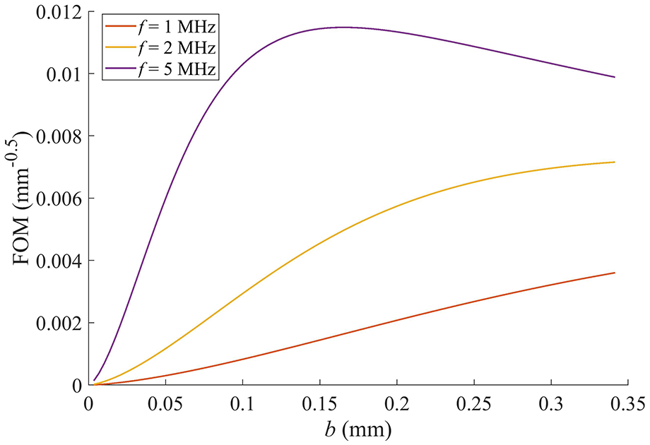
Typical FOM against half of grain size curves, plotted using equation (12) at frequencies 1, 2 and 5 MHz.
Grain size also has a significant impact on the attenuation. The grain size dependence of the attenuation has been discussed by Stanke and Kino.
36
It has been demonstrated that the attenuation coefficient is proportional to
Effect of defect size
In the following sections, examples are given for discussion. SNR maps of the examples are generated using the procedure introduced in section ‘SNR map generation’. As the inspection cylinder of a single transducer is always the target for an optimisation problem, the dependence of the cylinder parameters on various factors is of great interest and is discussed here.
Figure 7 shows a schematic diagram of an SNR map with an inspection cylinder of the same diameter as the transducer.
Schematic diagram of an SNR map.
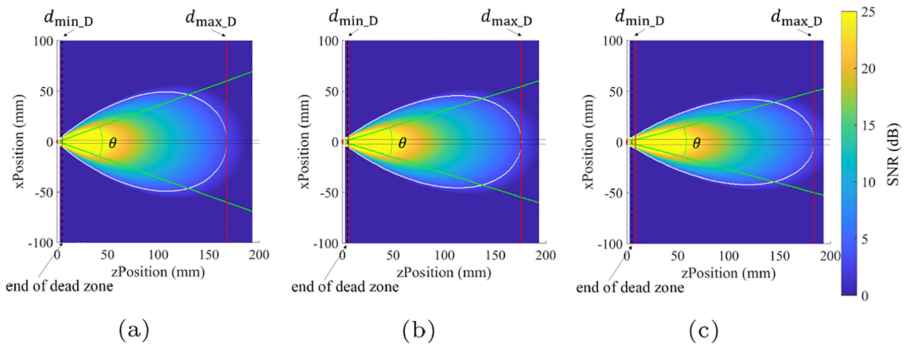
Next, how the divergence angle
Three defect diameters, 1, 2 and 5 mm, are considered for comparison. The anisotropy factor (Zener anisotropy factor
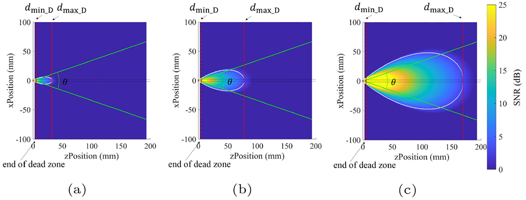
SNR maps (in dB) with defect diameters of (a) 1 mm, (b) 2 mm and (c) 5 mm.
It can be seen that the divergence angle
Effects of anisotropy factor
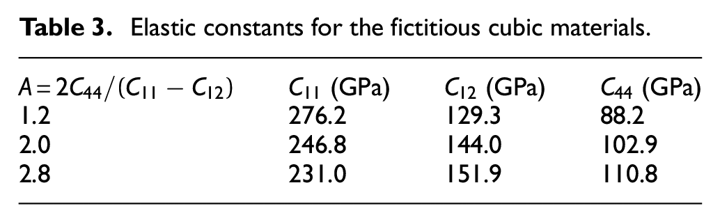
Next, the effect of anisotropy factor on the SNR is discussed. Three fictitious materials, which have the same Voigt velocity, Poisson’s ratio and density but have different anisotropy factors of 1.2, 2.0 and 2.8, are discussed here and their elastic constants are listed in Table 3. The defect diameter, transducer centre frequency and diameter are 5 mm, 1.8 MHz and 3.4 mm, respectively. The SNR maps are shown in Figure 9.
Elastic constants for the fictitious cubic materials.
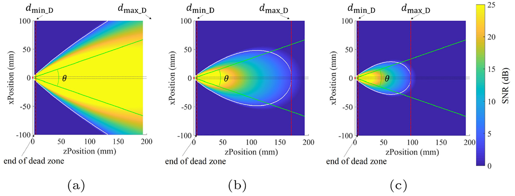
SNR maps (in dB) with anisotropy factors of (a) 1.2, (b) 2.0 and (c) 2.8.
It can be seen from Figure 9 that
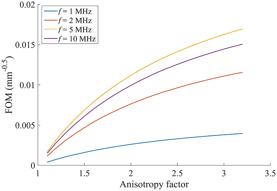
FOM versus anisotropy factor at frequencies 1, 2, 5 and 10 MHz obtained using equation (12). Each point shows the FOM calculated with the elastic constants which are obtained with the corresponding anisotropy factor.
Effects of transducer parameters
As the transducer frequency and diameter-to-wavelength ratio are usually the variables that can be modified to optimise the setup, it is of great importance to have a good understanding of their influence on SNR. Compared to the factors discussed in the previous sections, the transducer parameters have more complicated influence on SNR, as they affect the backscattering noise, the scattering amplitude of the defect, the scattering-induced attenuation and beam divergence. Therefore, the SNR maps are used to show their influence. This section begins with investigating the effects of the transducer frequency on SNR and then discusses those of the transducer diameter-to-wavelength ratio.
Three frequencies, 1, 1.4 and 1.8 MHz, are considered here. To keep
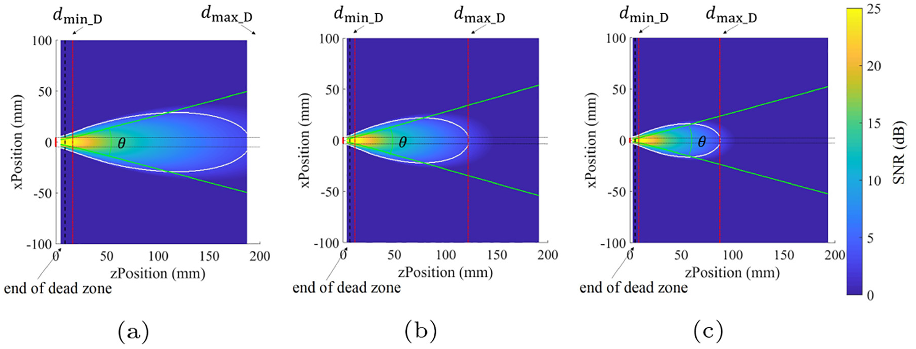
SNR maps (in dB) with transducer frequencies of (a) 1 MHz, (b) 1.4 MHz and (c) 1.8 MHz with a constant
It can be seen that the divergence angle
SNR maps (in dB) with transducer frequencies of (a) 1 MHz, (b) 1.4 MHz and (c) 1.8 MHz with a constant
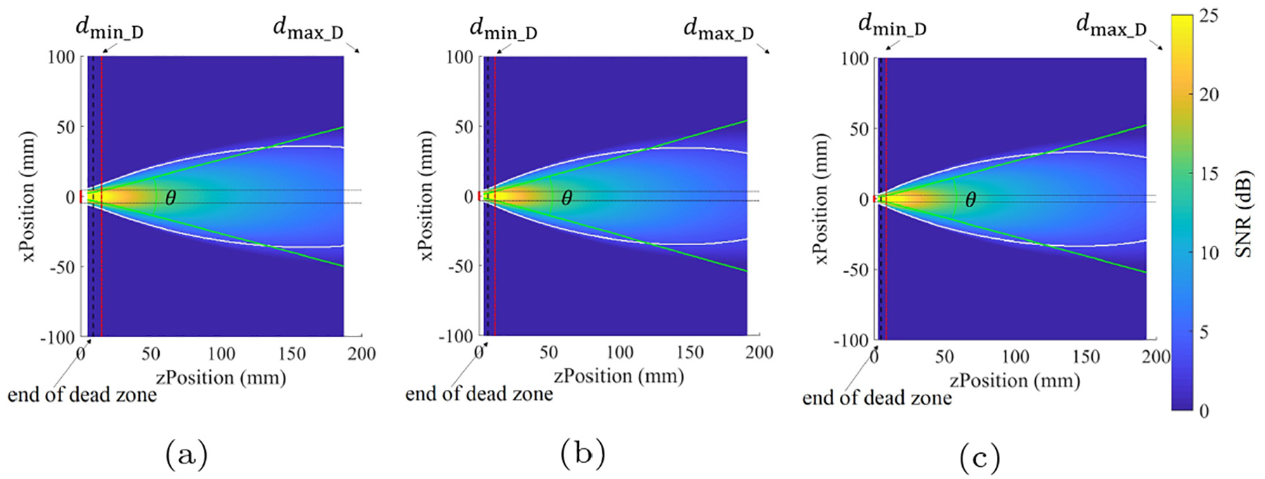
Next, the effects of the transducer diameter-to-wavelength ratio on SNR is investigated. Three ratios, 0.9, 1.2 and 1.5, are used here for discussion. The defect diameter, anisotropy factor and transducer centre frequency are 5 mm, 2.0 and 1.8 MHz, respectively. The SNR maps are shown in Figure 13.
SNR maps (in dB) with transducer diameters of (a) 3 mm, (b) 4 mm and (c) 5 mm. With a constant frequency of 1.8 MHz, the transducer diameter-to-wavelength ratios are 0.9, 1.2 and 1.5, respectively.
Figure 13 shows that with the increasing transducer diameter-to-wavelength ratio, the divergence angle
Summary
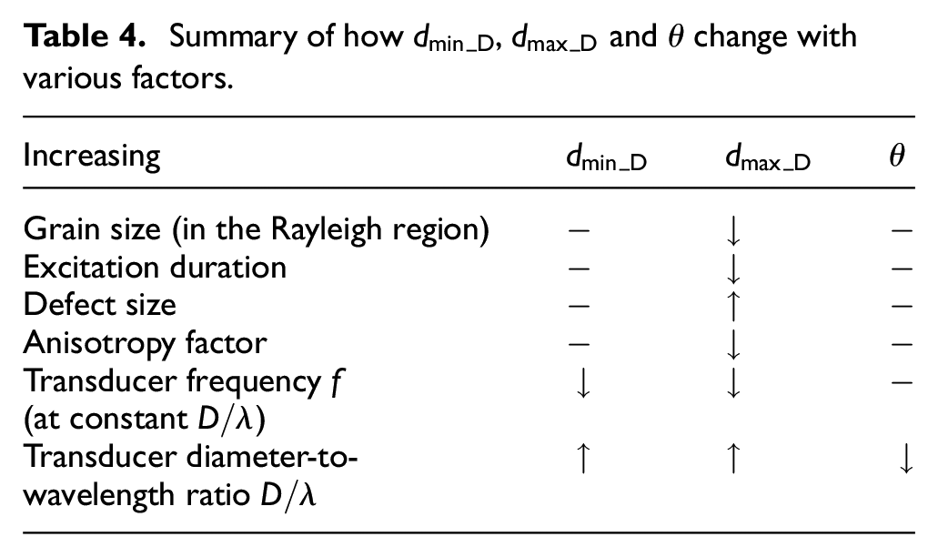
In this section, the influence of various factors on SNR has been investigated. It was shown that increasing the grain size (in the Rayleigh region), anisotropy factor, excitation duration or decreasing the defect size reduces the SNR. The SNR also decreases with increasing frequency (at constant transducer diameter-to-wavelength ratio), dominated by the scattering-induced attenuation. With an increasing transducer diameter-to-wavelength ratio (at constant frequency), the divergence angle decreases, which results in an increase in the SNR close to the centre line of the beam due to energy concentration.
The dependencies of the divergence angle
Summary of how
Case studies
All the requirements mentioned in section ‘Optimisation problem’ are considered in this section, the details of which are listed below:
The minimum SNR in the inspection cylinder is 3 dB;
The maximum radial SNR variation in the inspection cylinder is 6 dB;
The minimum transducer diameter
The minimum transducer diameter-to-wavelength ratio
The inspection cylinder diameter
The inspection cylinder is beyond the dead zone.
In this study, the optimal transducer parameters and placement are determined via comparing the SNR maps generated with multiple transducer frequency and diameter (
Next, two representative example optimisation problems, under each criterion respectively, are discussed and the results of the examples are illustrated with the trends obtained in section ‘Factors influencing the SNR’. Both of the examples consider a flat-bottom hole with a diameter of 2 mm in a fictitious cubic material of which the elastic constants (
Example 1
This section shows how to find the optimal
First, the minimum frequency and diameter–to-wavelength ratio are determined by the requirements. As the inspection cylinder should be able to cover the minimum depth of interest
Figure 14 shows the maximum depths of the inspection cylinders (in mm) obtained with different
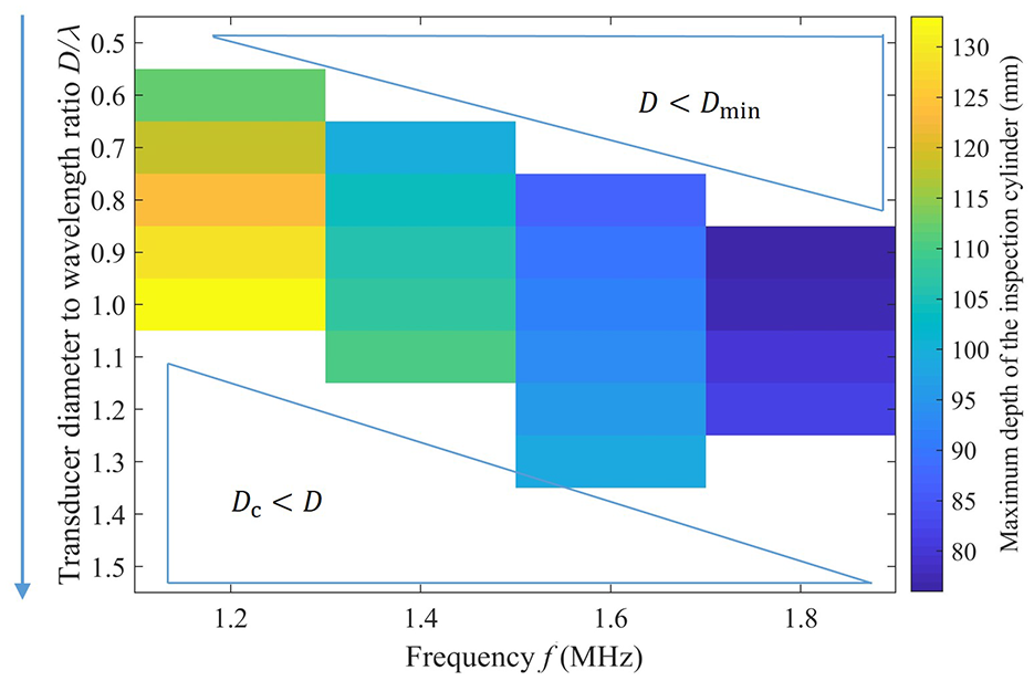
Maximum depths of the inspection cylinders (in mm) at different
From Figure 14, it can be seen that the optimal frequency and diameter-to-wavelength ratio are 1.2 MHz and 1, respectively, with which the maximum depth is 133 mm. The optimum is at a defect diameter-to-wavelength ratio of 0.4, so the approximation used in the calculation of the defect reflection is reasonable. From the parametric studies in the previous sections, it is known that the maximum depth of an inspection cylinder decreases with frequency, dominated by the scattering-induced attenuation, and increases with
Example 2
Next, another optimisation problem based on Criterion 2 with a depth range of interest from 95 to 105 mm is discussed.
With the same procedure described in Example 1, the SNR maps with multiple
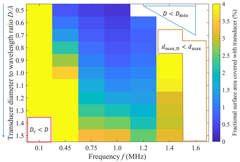
Fractional surface areas covered with transducers (
From Figure 15, it can be seen that the optimal frequency is 1 MHz and the optimal diameter-to-wavelength ratio is 0.5, with which
Experimental illustration
Example 2 shows how to obtain the optimal transducer parameters in the trade-off between volume coverage per transducer and sensitivity with a combined analytical and numerical method. In this section, a copper sample is monitored to illustrate this example experimentally.
The setup is shown in Figure 16. The dimensions of the sample are
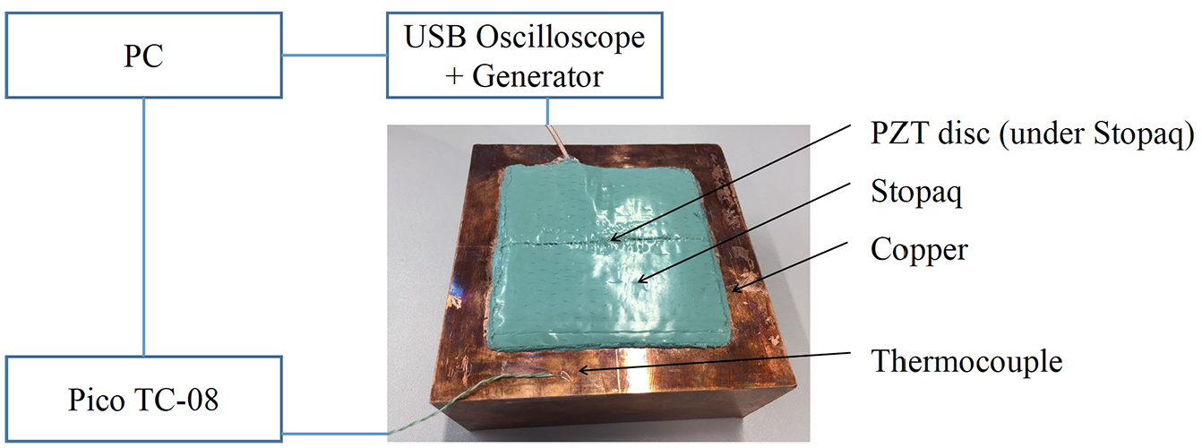
Experimental setup
As the transducer diameter is fixed, excitations of different centre frequencies were used to achieve different volume coverage and sensitivity. As the sensitivity is determined by various frequency-related factors, such as grain noise, defect reflection and attenuation, the relationship between frequency and sensitivity is relatively complicated. Here, as an illustration, the experiments are only used to investigate the relationship between frequency and volume coverage per transducer.
It is worth noting that the purpose of this section is to illustrate a key conclusion that the lower frequency transducer achieves wider beam spreading angles, rather than to demonstrate the whole method. The noise in the measured signals is largely due to the reverberation in the transducer assembly, though there is also noise coming from the scattering of copper sample. Therefore, the SNR is not further investigated using the proposed method, which considers the noise to be scattering-induced only.
Wave field measurement
In this section, the beam spread produced by the transducer is investigated. This can be achieved by measuring the signal amplitudes arriving at the bottom surface of the sample. The bonded PZT disc was used to transmit excitations and a contact transducer, with centre frequency 7.5 MHz and diameter 6 mm, was coupled to the sample surface opposite the PZT disc with a water-based gel to receive the signals. Eight measurements in which the receiver was recoupled to the surface were taken at each of eight locations uniformly distributed on the bottom surface between 0 and 35 mm from the centre line of the PZT disc; the multiple measurements ensured that coupling differences were minimised in the average results.
All the excitation frequencies were significantly below the disc resonance at around 8 MHz, so the response was centred close to the excitation frequency, and the received signals were first filtered around the corresponding excitation frequencies. The excitation used was a three-cycle Hann-windowed toneburst centred at 1, 2 and 3 MHz. With the 2- and 3-MHz excitation, the received signal had a similar centre frequency to the excitation and it was bandpass filtered at this frequency; since the 1-MHz excitation was far from the disc resonance, the response was centred at around 1.6 MHz and it was filtered at this frequency. The signal amplitudes are then plotted in Figure 17, where the points joined with straight lines show the mean and the errorbars show the standard deviation of the eight measurements at different locations. The measurements were collected within a short time period, therefore, the influence of temperature change is neglected.
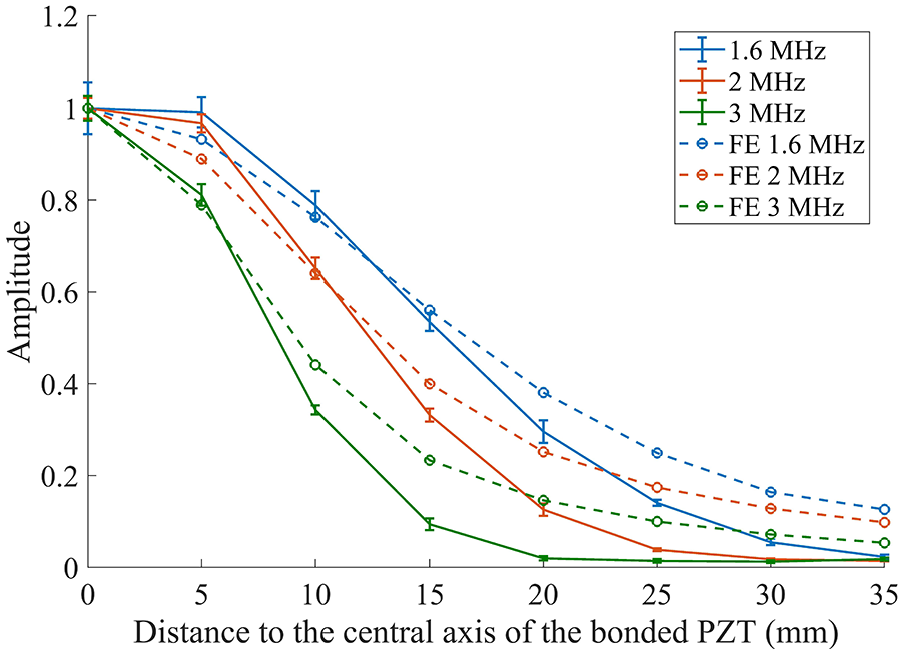
Normalised amplitudes of signals arriving at the bottom surface of the sample. FE results are shown with circle markers joined with dotted lines. The points joined with straight lines show the averaged experimental data of eight measurements at each location and the errorbars show their standard deviation.
FE simulations were carried out for validation. A 2D axisymmetric model was built in a similar way to that used in section ‘SNR map generation’, while the input parameters were set in accordance with the experiment. The materials of the PZT and bond line were the same as those used in section ‘SNR map generation’ and the copper was modelled as an isotropic material of which Young’s modulus, Poisson’s ratio and density were taken as 144 GPa, 0.324 and 9120 kg/m3, respectively. After filtering the signal in the same way as in the experiment, the FE results are shown with circle markers in Figure 17.
It can be seen from Figure 17 that the FE and experiment results show a similar trend. With lower frequency excitation, a wider beam can be obtained, which allows a larger volume coverage.
Defect reflection measurement
In this section, a pulse-echo configuration with the bonded PZT disc was used to measure defect reflections. Two flat-bottom holes, with the sizes and locations shown in Figure 18, were introduced to the copper sample, starting with the on-axis hole and then the off-axis one. Signals were collected every 10 min for 2 days before introducing the first hole and after the introduction of each of the two holes. This enabled baseline subtraction to be used to reveal the reflection from each defect.
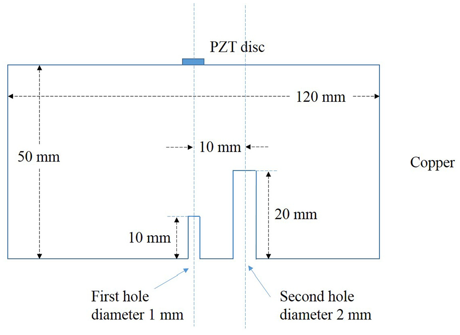
Schematic diagram of defect locations in the copper block with dimensions of
To remove the influence of the temperature change, only the signals collected at the same temperature 23.9°C are used in the following discussion. In practice, to compare signals collected at different temperatures, temperature compensation methods would be applied before baseline subtraction.11,38–40 The signals were first filtered in the same way as described in section ‘Wave field measurement’. Then the filtered signals collected with the undrilled sample, the sample with the on-axis hole and the sample with the two holes were averaged. Subtracting the averaged signal collected with the undrilled sample from that with the on-axis hole, the reflection from the on-axis hole can be obtained. Similarly, subtracting the averaged signal collected with the on-axis hole from that with the two holes, the reflection from the off-axis hole can be obtained.
Residuals containing the reflections from the on-axis and off-axis holes can be obtained at different frequencies, as shown in Figure 19. Reflections from the two holes can be seen in Figure 19(a) and (b) with relatively low frequencies and the amplitude ratio of the reflections from the off-axis hole to the on-axis hole decreases with increasing frequency. In Figure 19(c), only the reflection from the on-axis hole is visible, while that from the off-axis hole cannot be seen. This is consistent with the conclusion obtained in the wave field measurement, which is that with lower frequency excitation, a larger volume coverage can be obtained.
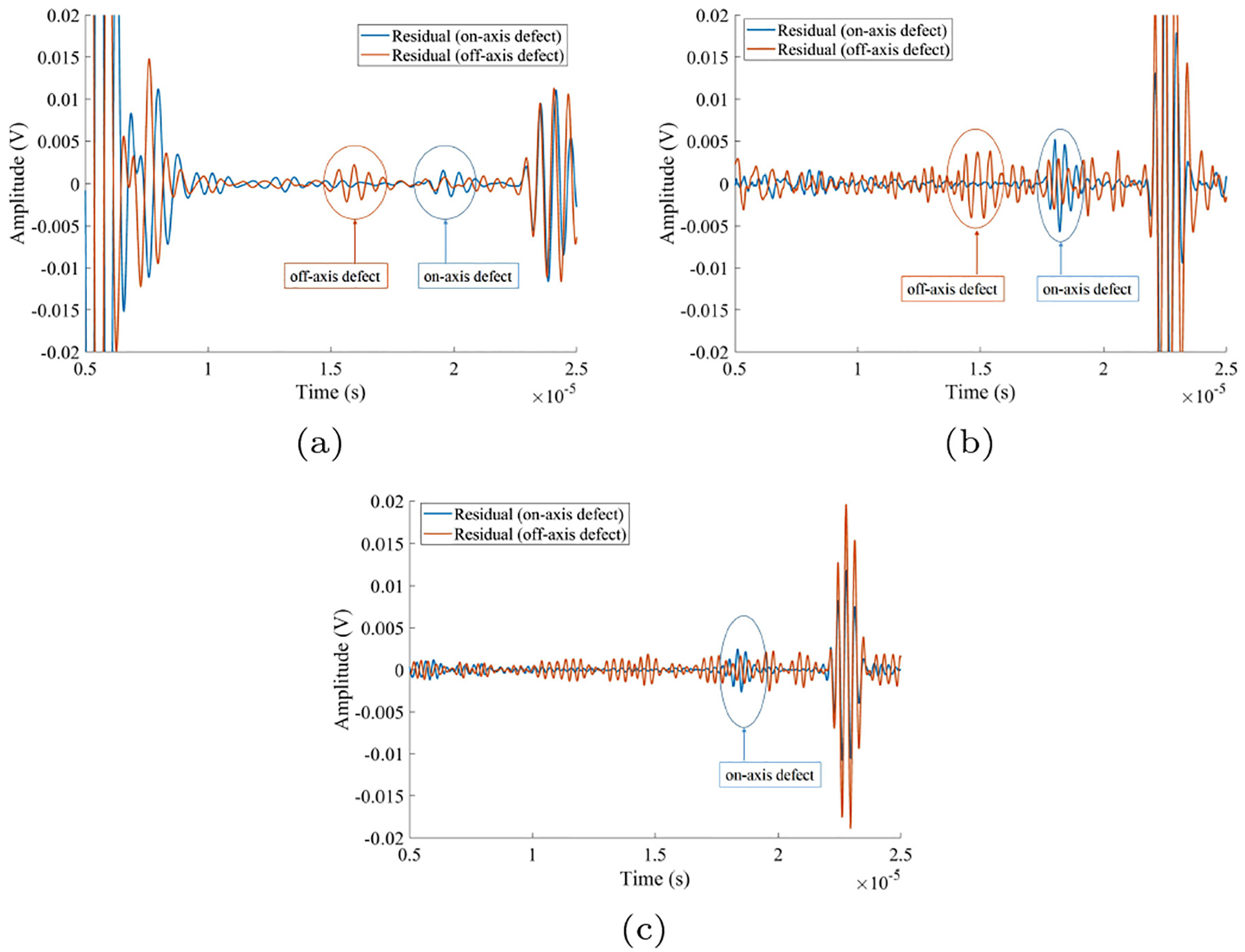
Residuals containing reflections from the on-axis and off-axis defects: (a) 1.6 MHz, (b) 2 MHz and (c) 3 MHz.
Conclusion
This article presented a design procedure for SHM systems based on bulk wave ultrasonic sensors for structures fabricated from polycrystalline materials. A challenge of monitoring coarse-grained polycrystalline materials is low SNRs caused by grain scattering. Therefore, when designing an ultrasonic monitoring system for structures fabricated from these materials, in addition to a general requirement of maximum coverage per transducer, sufficient sensitivity throughout the monitoring volume is an important requirement. The trade-off between volume coverage per transducer and sensitivity has been introduced and investigated, and a methodology using signal-to-noise maps has been presented to determine the optimal frequency, diameter and placement of the transducers.
A combined analytical and numerical approach has been used to generate a signal-to-noise map and the influence of various factors on SNR has been discussed. It is found that the SNR decreases with increasing grain size (in the Rayleigh region), anisotropy factor, excitation duration and decreasing defect size. Increasing the frequency (at constant transducer diameter-to-wavelength ratio) reduces the SNR, dominated by the scattering-induced attenuation. Increasing the transducer diameter-to-wavelength ratio (at constant frequency) decreases the divergence angle, which results in an increase in the SNR close to the centre line of the beam due to energy concentration.
Two representative examples, with different criteria, have been given to illustrate the methodology. One example aims to achieve the deepest range with the full surface area of the testpiece covered with transducers and the other one aims to achieve the minimum fractional surface area that has to be covered with transducers to monitor a narrow depth range far from the surface, which has a potential application in weld monitoring. It is found that if regions close to the top surface are to be monitored, a relatively high frequency is needed to limit the dead zone. If a large depth needs to be covered, a low frequency, to reduce the attenuation, and large transducer diameter-to-wavelength ratio, to concentrate the energy, should be used. For modest scattering, a narrow depth range far from the surface can be monitored with a small surface area covered with transducers, which has potential application in weld monitoring. For highly scattering materials and large inspection depths, a low frequency is required to reduce the attenuation and the depth range can be increased by increasing
Only the pulse-echo configuration is discussed in this article, but the methodology of the optimisation has the potential to be generalised to a pitch–catch problem with the theoretical model given by Thompson and Gray. 19 It is worth noting that the pitch–catch mode of operation would require that the transmitter and receiver beams overlap each other, therefore the optimisation would be not only more complex but also would target a very different optimum between coverage and SNR. In addition, for a pitch–catch system, it is required that the transmitters and receivers must be synchronised; this is easy to achieve if they are wired together, but much more difficult if they are independent wireless units.
Footnotes
Declaration of conflicting interests
The author(s) declared no potential conflicts of interest with respect to the research, authorship and/or publication of this article.
Funding
The author(s) disclosed receipt of the following financial support for the research, authorship and/or publication of this article: This work was supported by the Engineering and Physical Sciences Research Council via the UK Research Centre in NDE (grant no. EP/L022125/1).