
Abstract
Many approaches at the forefront of structural health monitoring rely on cutting-edge techniques from the field of machine learning. Recently, much interest has been directed towards the study of so-called adversarial examples; deliberate input perturbations that deceive machine learning models while remaining semantically identical. This article demonstrates that data-driven approaches to structural health monitoring are vulnerable to attacks of this kind. In the perfect information or ‘white-box’ scenario, a transformation is found that maps every example in the Los Alamos National Laboratory three-storey structure dataset to an adversarial example. Also presented is an adversarial threat model specific to structural health monitoring. The threat model is proposed with a view to motivate discussion into ways in which structural health monitoring approaches might be made more robust to the threat of adversarial attack.
Background
Data-driven modelling in structural health monitoring
Monitoring the health of engineering structures is of critical importance to countless engineering disciplines and applications. Since it is very difficult for most sensors to measure damage, 1 the practising engineer must instead rely on a range of indirect tools and techniques in order to identify, locate and manage damage in structures.
Much interest in the field of structural health monitoring (SHM) has been in data-driven approaches that leverage techniques from machine learning and statistical pattern recognition. 2 Several authors have extolled the virtues of casting SHM problems in this way.3,4 The modern engineer is fortunate to have at their disposal a litany of tools that are able to perform pattern recognition, and the literature reflects this. To date, authors have employed outlier analysis, 5 neural networks, 6 support vector machines 7 and decision trees 8 among many other approaches. The reader is directed to Farrar and Worden 9 for a comprehensive reference text.
Despite the wealth of progress made in the last two decades, the large-scale deployment of SHM methodologies is still in its infancy. There are many well cited reasons for this, with the scarce availability of damaged training data and issues surrounding environmental variation emerging as key themes. However, innovative solutions to these problems are steadily being found.
In the face of these challenges, there are several large-scale systems that are currently in deployment. Perhaps most famous is the OnStar navigation and diagnostics system available in some commercial vehicles. There is also the integrated condition assessment system (ICAS) 10 deployed by the US navy for the monitoring of hardware, as well as a number of techniques developed for monitoring rotor-craft under the umbrella term of health and usage monitoring systems (HUMS). 11 These systems are all implemented in potential life-safety applications and are therefore potential targets for malicious attack.
It is the opinion of the authors that if SHM frameworks are to be adopted in life-safety or economically critical projects, then it is of utmost importance that the security and robustness of the underlying models are rigorously examined.
Adversarial attacks on pattern recognition models
It is important here to distinguish between the similar but distinct topics of adversarial attack and adversarial machine learning. The latter refers to machine learning methods whereby two learning models are pitted against each other in order to produce generative models 12 that are able to sample from the underlying input distributions.
Adversarial attack, however, refers to the construction of adversarial examples for classification models. These are deliberately perturbed inputs for which the classifier assigns an incorrect label despite small or imperceptible semantic alteration from the true state. Mathematically, for a classification model

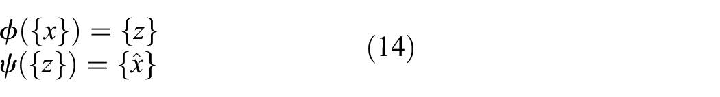
An adversarial example

The adverse label is assigned despite semantic similarity to a human observer

The vulnerability of neural-network models to adversarial attack was first presented by Szegedy et al. 13 It was later shown that the vulnerability of such models was not limited to the area of neural networks. 14 In fact, a wide array of classification algorithms are susceptible to this type of attack. Subsequently, Carlini and Wagner 15 produced a general approach for the construction of adversarial examples that were difficult to detect and were able to bypass several of the recently proposed adversarial defence strategies.
Since this revelation, the literature has grown rich with contributions exploring adversarial attacks and the generation of adversarial examples. A recent review can be found in Yuan et al. 16 By far, the majority of the case studies and the application papers thus far published on adversarial attack have been concerned with image classification and machine vision. It is in these areas that the majority of the taxonomy has been developed. In this article, the authors hope to demonstrate that adversarial attack is also a real threat to SHM models.
Data-driven approaches to SHM rely at their core on machine learning models that are susceptible to adversarial attack. While some of these rely directly on neural networks,6,17–19 Papernot et al. 14 demonstrated extensively the vulnerability of techniques beyond neural networks, including support vector machines, decision trees, logistic regressors and others in their highly cited paper. With this in mind, it is clear that the adversarial attack is a threat to a great deal of data-driven SHM.
While no direct consideration of adversarial vulnerability for SHM has yet been presented in the literature, the susceptibility of data-driven approaches has already been demonstrated for the related field of process monitoring. 20 In their paper, the authors demonstrate the adversarial fragility of a deep neural network trained to detect system failures and offer an adversarial training method similar to Madry et al. 21 for hardening the classifier.
With the rapid pace of adversarial attack research in mind, it is the aim of this article to motivate serious discussion into the vulnerability of the learning models proposed for SHM. Presented here are two contributions. The following section envisages an adversarial attack threat model for SHM. The threat model is accompanied by a taxonomy specific to threats arising in SHM frameworks. The third and the fourth sections provide demonstration of adversarial attack on a damage detection model trained on an SHM-benchmarking dataset. It is shown that simple transformations can be constructed that map every true input to an adversarial example, even when the inputs have not been used to train the classification model. The final section outlines the directions for further investigation into ways in which SHM might be made more robust to adversarial attack.
An adversarial attack threat model for data-driven SHM
The foundation for this threat model will be the vibration-based damage identification framework presented in Farrar et al. 22 The approach can be summarised by four steps:
Operational evaluation
Data acquisition
Feature extraction or pre-processing
Label discrimination
This framework is expanded in Figure 1 to produce a physics-to-label representation of the SHM framework. For convenience, the following definitions are presented:
A SHM framework (the system, Figure 1) that utilises a statistical pattern recognition model (the model,
A malicious entity (the attacker) is attempting to influence or compromise the accuracy of the model by leveraging adversarial examples ({x′}) to induce false or misleading results.
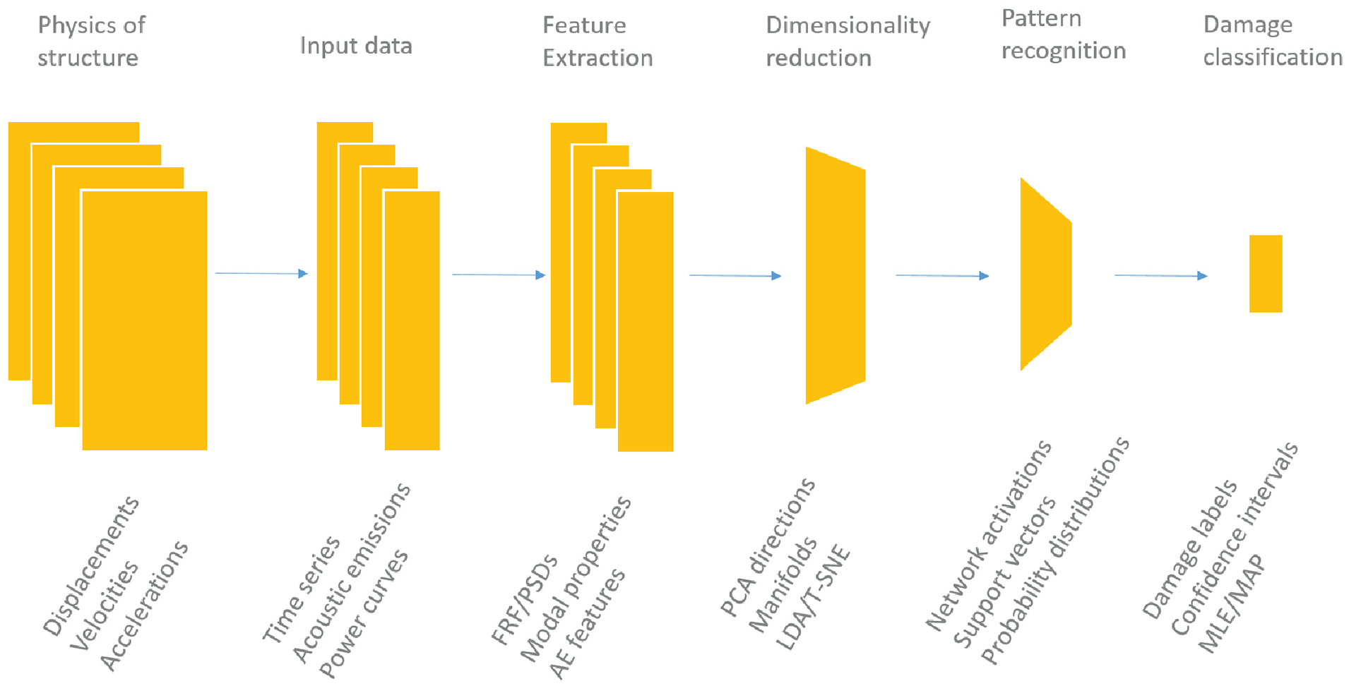
An example overview of a data-driven SHM methodology.
The principal threats in this scenario are thus defined as follows:
The false labelling of the damaged state as undamaged (false negative,
The false labelling of the undamaged state as damaged (false positive,
Semantic similarity between real and adverse inputs to the model
Thus, we may define a general objective function for the production of semantically convincing adversarial examples as

where
The consequences of a false-positive classification may seem minor compared to that of the false-negative classification and in the extreme this is certainly the case. However, unnecessary maintenance and inspection may bear a financial toll and repeated miss-classifications may erode confidence in the monitoring system. Unaddressed, either of these eventualities are likely to render the system completely useless in the long term. Furthermore, if the adversarial examples have high semantic similarity to measured healthy data, it would be very difficult for a human to recognise the occurrence of the adversarial examples and troubleshooting the problem may be difficult.
The SHM analogue of semantic similarity from image recognition is not immediately intuitive. It is unlikely that a human would be able to identify damage by observing measured signals from a structure alone. However, there are domains that do present semantic information to the trained eye. For intuition, consider the frequency response functions (FRFs) of a vibrating structure. FRFs are frequently used as damage and condition-sensitive features in SHM as they encode physical dynamic properties and can be efficiently computed. To a trained engineer, the natural frequencies and damping properties of a structure are approximately tractable visually and it would certainly be possible to identify significant deviation from the expected structure of the signal. FRFs, as well as other features such as coherence and acoustic emission signals, contain semantic structure and are all potential targets for adversarial attack.
Threat model
In order to arrive at a coherent adversarial attack threat model for SHM, it is important to first consider the vectors for attack that are present in the system. Figure 2 presents a breakdown of the principal attack vectors into three domains.
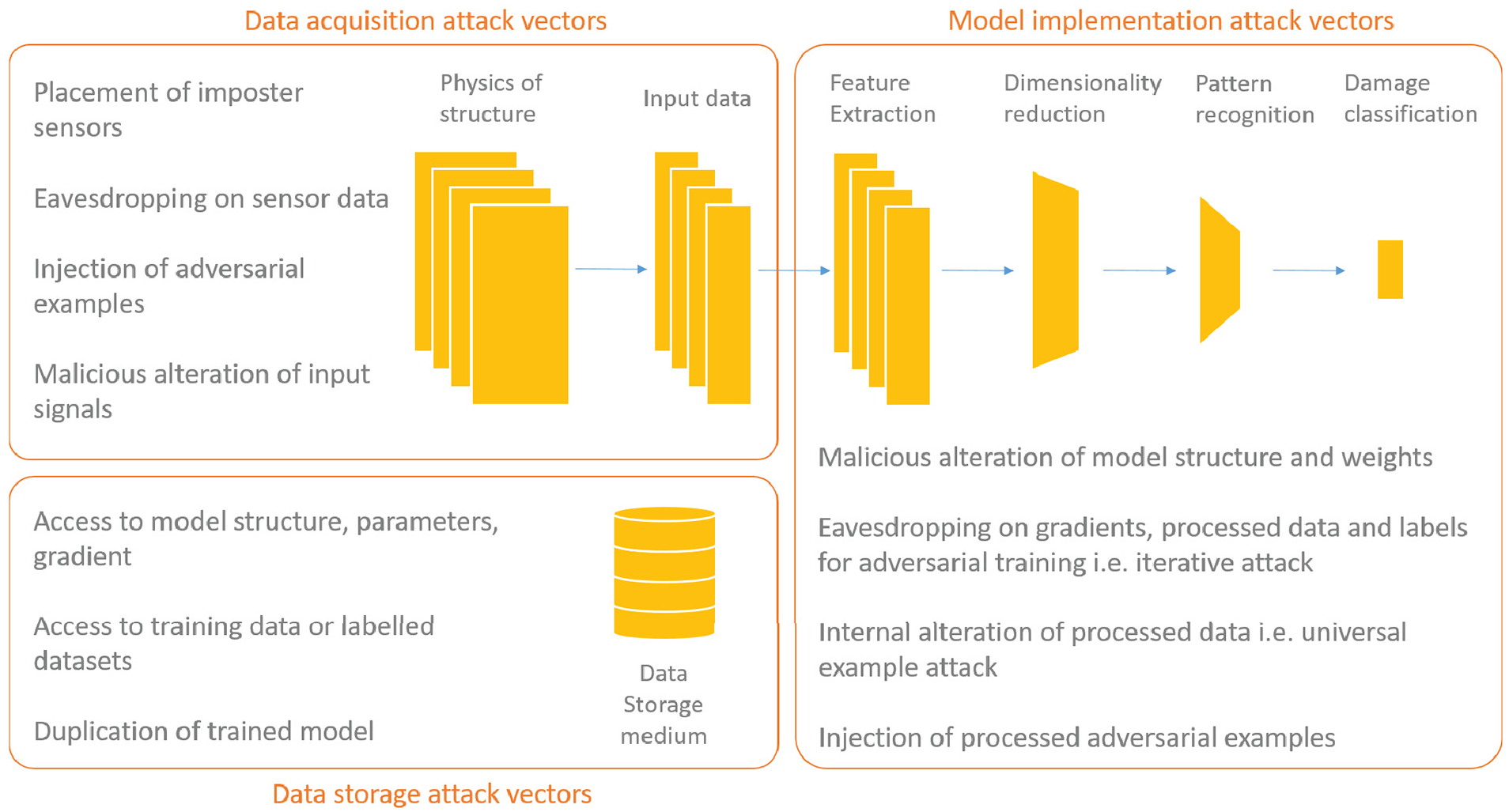
Categorisation of attack vectors.
The first of these is the data-acquisition domain and is largely concerned with the physical security of sensing equipment. Given access, the attacker is able to adversely influence or gain access to structural measurement data. This includes both online data collection and training data collection. Vectors for attack include the placement of impostor sensing equipment, ‘spoofing’ sensors with adversarial inputs and eavesdropping on sensor data.
The second domain is related to data storage security. Threat models for generic data storage security have been previously explored in Hasan et al. 23 In the context of SHM, the principal threat is that training and model data might be maliciously accessed with the intent to construct adversarial examples. A data breach could arise as the result of either a physical or cyber intrusion and so hardening the system to these vectors is especially difficult.
The third domain is concerned with the implementation of the model. The principal threat is that knowledge of the structure and parameterisation of the model might become available to the attacker. Risks in this domain are largely concerned with insider threats, whereby a person with trusted access to the implementation and acquisition components of the system is able to act maliciously. However, other means of access, such as social engineering and espionage, are also vectors by which access to model implementation might be acquired. With total access to the system, an attacker would be trivially able to bypass safeguards and affect their machinations.
Threat taxonomy
In light of the earlier discussion, the principal distinction between adversarial attack types is the level of access that is afforded to the attacker. This is certainly the case in the machine learning literature where attacks are characterised as either white- or black-box.
In a white-box attack, it is assumed that the attacker has complete access to the system. This could include model structure, parameters and gradient information, as well as access to the training data, inputs and outputs. This corresponds to access in all three domains of Figure 2. The white-box attack is primarily a simulation of the insider threat. The scenario can also apply to systems whereby the implementation has been made publicly available, for example, if the model had been published in the academic literature.
In a black-box attack, it is assumed that the attacker has query access to the model only, with no knowledge of the model structure, training procedure or access to a training dataset. There is some variation in exactly what is available to the attacker in the literature. Papernot et al. 24 assumed that a very small set (less than 10 per class) of examples from the input domain (but not necessarily the training data) are available. In an SHM context, we include scenarios whereby the attacker is able to query the model and has access to incoming data as black-box attacks.
The black-box attack is indicative of an outsider threat whereby an attacker is able to query the classifier either remotely via a cyber attack or by gaining access to models and data during a physical attack. In order for the black-box attack to be realistic, the number of queries to the classifier must be kept to a minimum. Guo et al. 25 argued that any black-box attack that makes use of many thousands of queries can easily be defeated by query limitation.
Consideration of both the white- and black-box scenarios is important for SHM applications. One question the SHM community is going to have to deal with is how to certify SHM systems for monitoring publicly owned critical infrastructure for life-safety applications. The importance of this issue will increase as SHM research has begun to mature and SHM systems begin to be sold commercially. The complexity of SHM systems is high enough that the community itself will need to provide public authorities guidance to guard against commercial entities selling malicious or sub-standard SHM systems. One way to guard against the use of sub-standard SHM systems is to mandate that the design of these systems be transparent. However, transparency is often not in the interest of commercial entities, and it does make white-box attacks more easy to execute. This tradeoff between security and ensuring the performance of SHM systems must be considered. Furthermore, as 5G networks become more prevalent, they will increasingly be used to implement SHM systems. A number of security risks have been identified with 5G networks (e.g. supply chain, interdependencies and increased overall attack surface) that make white-box attacks more plausible. 26 As a result, both white- and black-box scenarios should be considered by the SHM community.
Based on the original work on adversarial examples, 13 a great number of approaches have been developed for the construction of adversarial examples. The recent review by Yuan et al. 16 does an excellent job in recording and categorising the approaches that have thus far been proposed. A brief outline of the key definitions is included here.
Attack scope
An example search is a style of attack that performs optimisation in the input space of the SHM model to specify single or multiple adversarial examples ({x′}) that are optimised independently. This type of attack is most likely to be enacted as a one-time attack.
A training attack (also referred to as data poisoning) is conducted during the training phase of the SHM framework, before the system has been fully implemented. During a training attack, the training data are augmented or appended with adversarial examples with a view to maximise erroneous classification within the model itself.
A universal example search is an altogether different type of attack. Instead of optimising individual examples, the attack is a search for a function


This is often a more challenging task (as the mapping must span the input space) and is more dangerous to the operation of an SHM system as the adversarial examples can be delivered continuously in an online fashion.
Adversarial specificity
In a targeted attack, the adverse class labels are specifically chosen such that, for example, a damaged structure is selectively labelled as undamaged
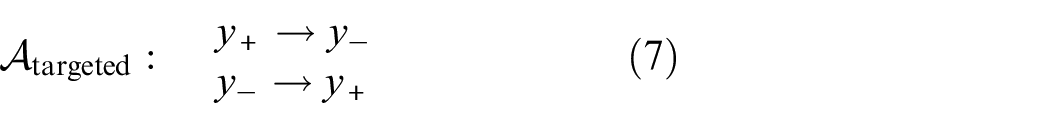
In an untargeted attack, there is no specific attention paid to which label is assigned to the adverse example as long as it is not the true class. In the binary classification case, this is equivalent to the targeted attack

Attack frequency
A one-time attack involves the specification and injection of adversarial examples without querying the classifier. Such attacks might be appropriate for attack motives that require only temporary falsification of the SHM system.
An iterative attack makes multiple queries to the classifier to assess the effectiveness of the adverse examples, improving their potency iteratively. This attack style tends to result in more semantically convincing examples but comes at the cost of increased computational effort and risk of exposure.
Dataset and classification results
This section details the specification and training of a classification algorithm for the Los Alamos National Laboratory (LANL) three-storey structure dataset (Figure 3). 27 The primary objective of the classifier will be to accurately predict damage labels despite the presence of simulated environmental variation.

Schematic view of the three-storey structure (all dimensions are in cm).
There are essentially two classes of algorithm available for performing this task. Generative models aim to construct the full joint probability of the labels and the data. The advantage is that the algorithm is able to return predictive probability distributions and so uncertainty in the predictions is handled graciously.
By comparison, discriminative models aim to reconstruct only the class conditional probabilities and so only the labels themselves can be returned. For this work, only discriminative models are considered.
LANL three-storey structure dataset
The three-storey structure was conceived as a test-bed for SHM algorithms. Many published approaches to SHM demonstrate their effectiveness on this dataset. This prominence in the literature makes the three-storey dataset ideal for demonstrating the vulnerability to adversarial attack. Another objective of the original report on the dataset is to assess robustness in the face of environmental and operational variation. As such, there are 17 structure configurations (detailed in Table 1) representing either a damaged or undamaged state.
The 17 structural states recorded in the LANL three-storey dataset.
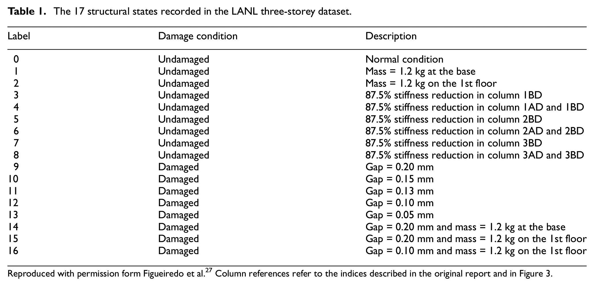
Damage is simulated in the structure by the inclusion of a bumper that acts between the second and third storeys of the structure. The impacting bumper adds significant nonlinearity to the dynamics of the structure. The gap, measured from the equilibrium point to the bumper, is varied to simulate the progression of damage. The bumper engages once the inter-storey displacement exceeds the gap distance. This means that smaller gap distances simulate increased levels of damage. A full account of the configuration of the structure in each of the 17 states is recorded in Table 1.
The dataset consists of the input force and acceleration responses measured at each storey of the structure. The structure is excited with a band-limited (20–150 Hz) Gaussian forcing signal by an electrodynamic shaker attached to the base. The data are recorded with 50 tests per state where each test consists of 8192 points recorded at a sampling frequency of 320 Hz. In order to increase the number of examples available for training the classifier, each of the tests are divided in half, resulting in 100 tests per state of 4096 points (1700 examples in total).
Classification approach
As state labels are available for the dataset, the classifier will be trained in a supervised manner. The extracted features will be the accelerance FRFs estimated by the Welch method (resulting in a real-valued spectral density) with no overlap, the Hanning window and five-fold averages. FRFs are computed for the base of the structure and each for of the three-storeys.
The FRF for the ith storey
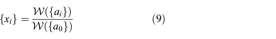
where
The use of FRFs as features is motivated by the observation that variations in the normal condition (masses, stiffnesses) exhibit more variance in the natural frequencies of the spectra, whereas the damage progression is most evident in the variance of the higher frequencies. The FRF is therefore a suitable feature as it is independently expressive in both of these directions.
For further motivation and in order to aid visualisation, Figure 4(a) and (b) depict the first two principal components of the dataset for the time series and the FRFs, respectively. The individual classes are clearly more separable in the FRF basis. In addition, variations in normal condition seems to be approximately orthogonal to the progression of damage. Figure 5 shows the first two principal components of the FRFs recoloured to depict damage labels only.
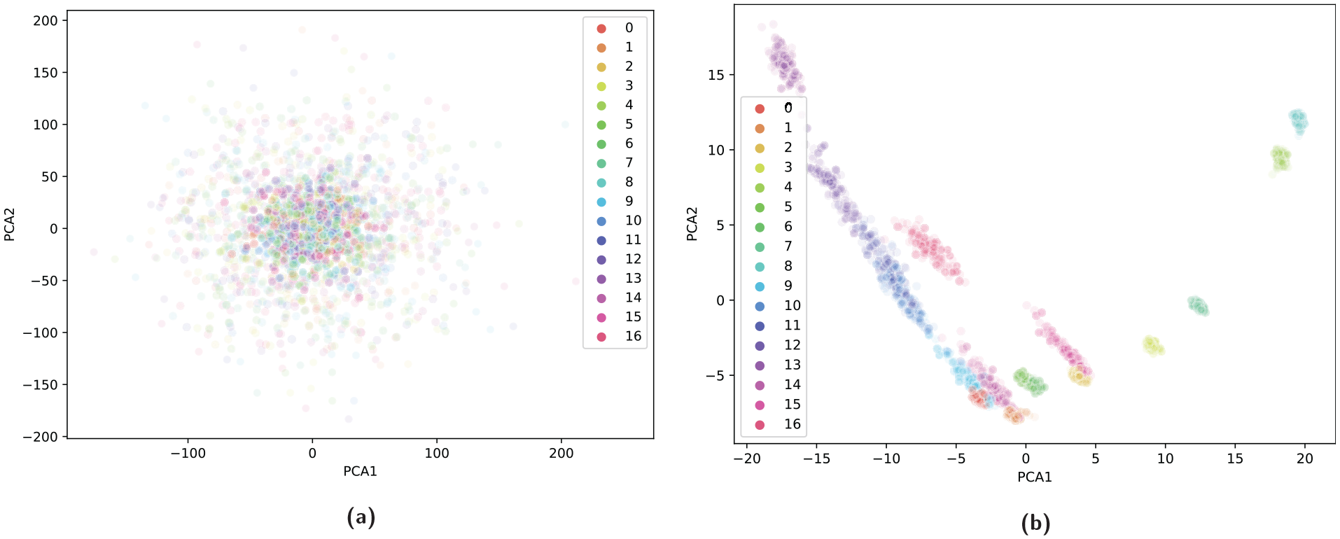
Comparison of label-sensitive features: the first two principal component directions plotted and coloured by label. Label clusters are visually far more separable in the FRF domain: (a) time series data and (b) FRF data.
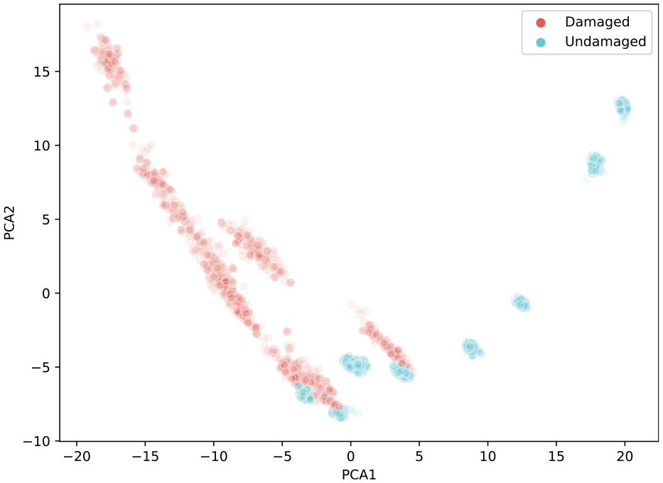
First two PCA components of the FRF data, recoloured to reflect damage labels.
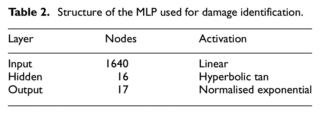
For the task of damage identification, a multi-layer perceptron (MLP) is trained with a single hidden layer. The structure of the classification model is detailed in Table 2. The dataset is divided into training and validation sets with 500 examples separately reserved for the evaluation of performance on unseen examples.
Structure of the MLP used for damage identification.
The network is initialised with random weights uniformly distributed on the interval [–1, 1] and then trained for up to 100 epochs using a cross-entropy loss function and the Adam optimiser. The hyperparameters for the optimiser are set to the default values provided in the original study. 28
The training process is repeated for hidden node numbers in the range [1, 100]. Figure 6 depicts the training curves for training and validation sets. The figure clearly depicts a stable training regime with excellent validation performance on networks with greater than around 15 hidden nodes. Although many network structures give optimal performance, in order to ensure our demonstration is as realistic as possible, the simplest model with the best validation accuracy is selected. This is a network that achieves a validation accuracy of 99.58% with 16 hidden nodes trained over 79 epochs. The structure of the classification model is detailed in Table 2.
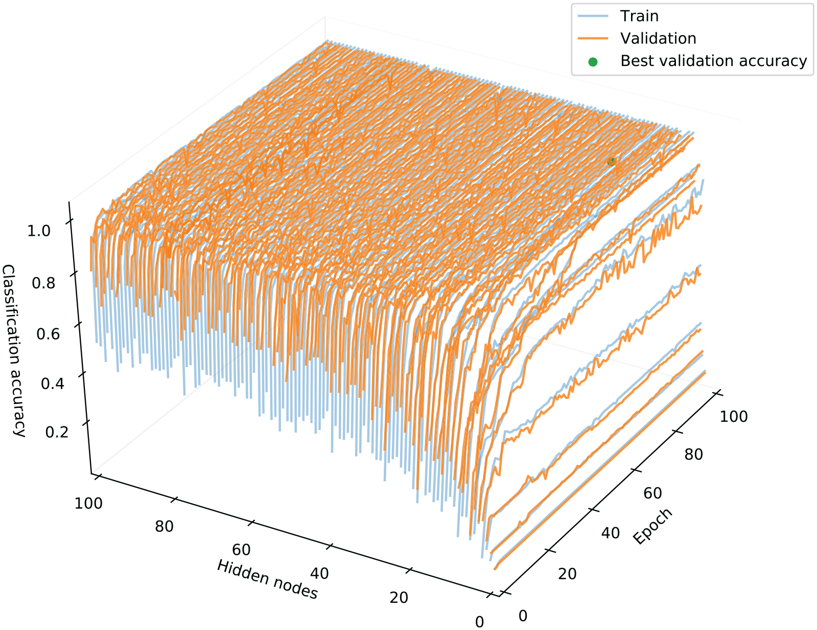
Training curves for the classifier, varying the number of hidden nodes.
Classification results
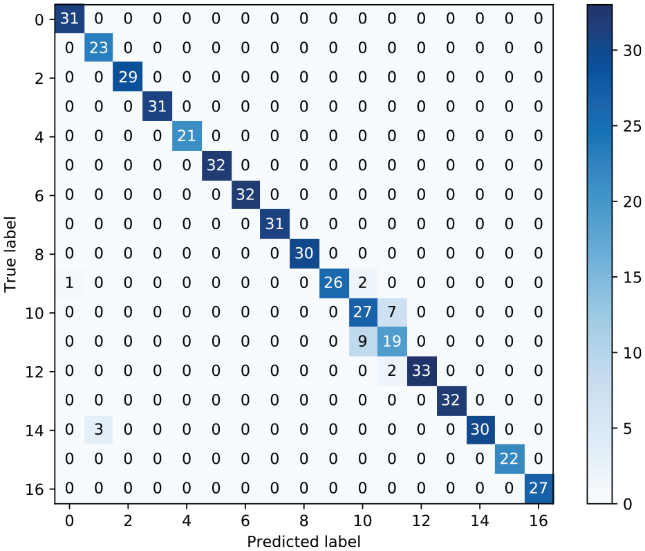
Figure 7 depicts the classification confusion matrix on the 500 unseen testing examples that were not used during training. The classifier achieves a multi-class prediction accuracy of 98.60% on the testing data, with only two (0.40%) false-positive and zero false-negative classifications. The remaining miss-classifications (1.00%) are between the three damage classes that have the smallest geometric differences in gap size.
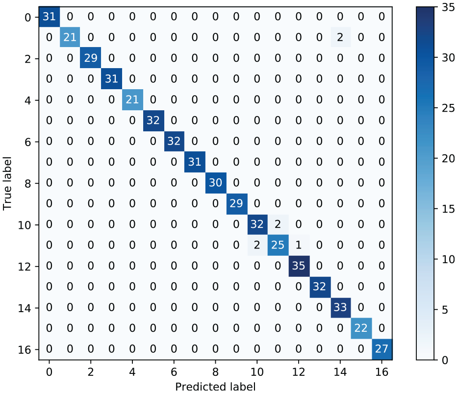
Confusion matrix of the classifier on unseen testing data.
Conventional analysis of the capacity of classification models such as the Vapnik–Chervonenkis (VC) dimension 29 places lower bounds on the number of training examples required to ensure generalisation. However, empirical evidence and recent studies 30 show that neural networks and deep learning models routinely outperform the theoretical limits placed on them. Such models are often shown to achieve strong empirical generalisation despite enormous VC-dimensions and limited training data.
The dataset used here is small (1700 examples) compared to the number of examples in modern deep learning benchmark problems (typically on the order of 100,000 examples) and indeed the VC-dimension of the model (a simplified estimate would be
Demonstration of adversarial vulnerability
The objective of this article is to motivate serious discussion into the vulnerability of data-driven SHM models by demonstrating the most threatening attacks in both the white-box and black-box threat scenarios. For brevity, we consider only the more challenging task of performing a universal example search. The goal is to identify an adversarial transformation

where
For maximum impact, the demonstration is conducted as a targeted attack. The approach here is the more challenging task of aiming for perfect miss-classification with every label representing either a specific false-positive or false-negative result. Adverse training labels are constructed by the following targeted scheme
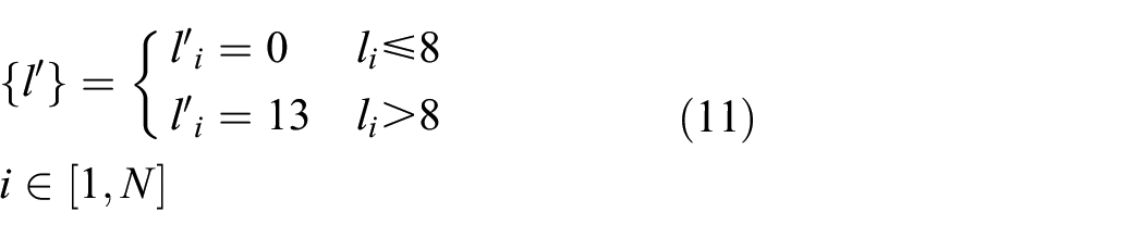
where N is the number of training examples. A class label of zero corresponds to the normal condition, whereas a class label of 13 relates to the maximally damaged state. Constructing the adversarial target labels in this way ensures that
Demonstration of white-box attack
The first demonstration of adversarial attack on an SHM implementation is conducted in a white-box manner. Since gradient information is available in this context, the parameters of the adversarial transformation
For the white-box demonstration, the adversarial transformation
The second phase is the learning phase during which the network learns a perturbing transformation that maps true inputs to adversarial examples. The exact procedure is as follows. During the listening phase, an MLP (Table 3) with parameter set
where
Parameters of the MLP used for adversarial perturbation.
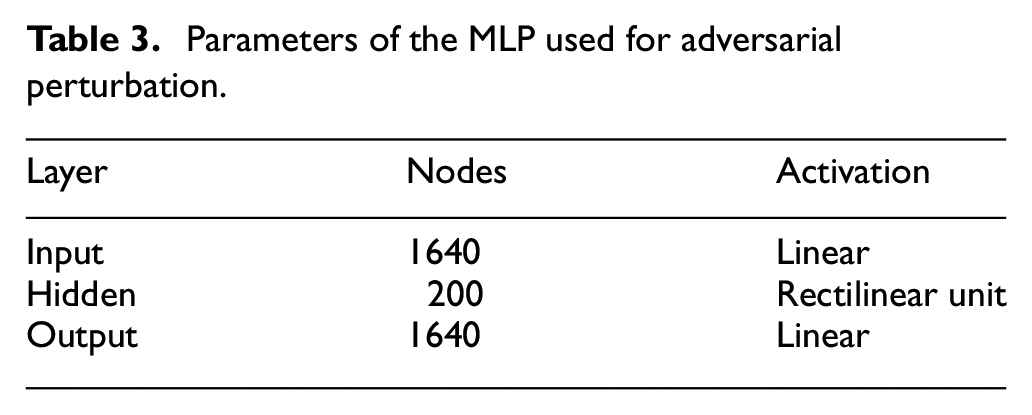
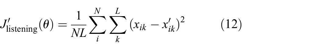
During the learning phase, training is conducted as a multi-objective problem with constraints placed on both the cross-entropy loss between the predicted and adversarial labels and the mean-squared error between the adversarial example and the true output
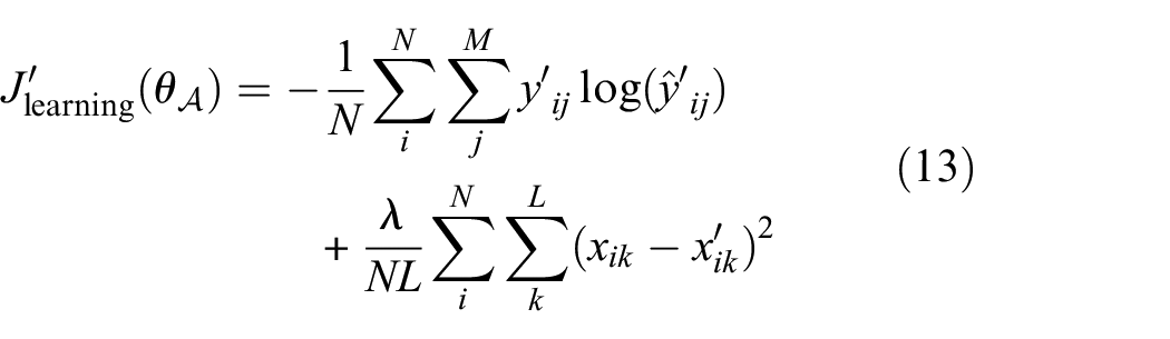
where M is the number of classes in the dataset and L is the dimension of the input. The parameter
In order to verify that the attack has been successful, the testing set of examples not used during adversarial training is fed through the perturbing network and classified. Figure 8 depicts the confusion matrix of the classifier on the adversarially perturbed validation examples. The confusion matrix represents 99.58% and 100% as false-negative and false-positive classification rates, respectively. In fact, only a single example was correctly assigned a damage label by the classifier. The adversarial transformation has rendered the SHM classifier useless.
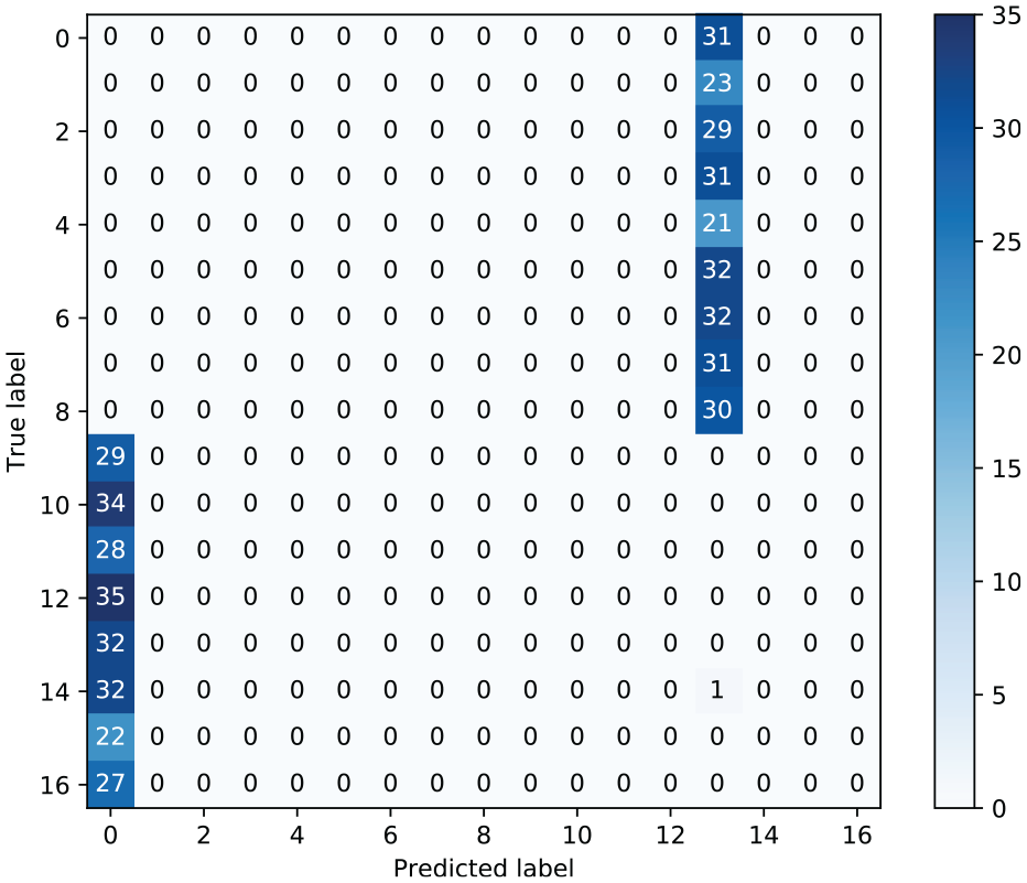
Confusion matrix of the classifier during a white-box attack.
Figure 9 plots the resulting adversarial examples from the false-positive and false-negative cases, respectively. Looking at the adversarial examples, it can be seen that there is a high level of semantic similarity between the adversarial and true signals. This is especially pronounced in the false-positive examples which are almost indistinguishable from the unperturbed input. It seems that the largest semantic differences are present in the variance of the false-negative adversarial examples.
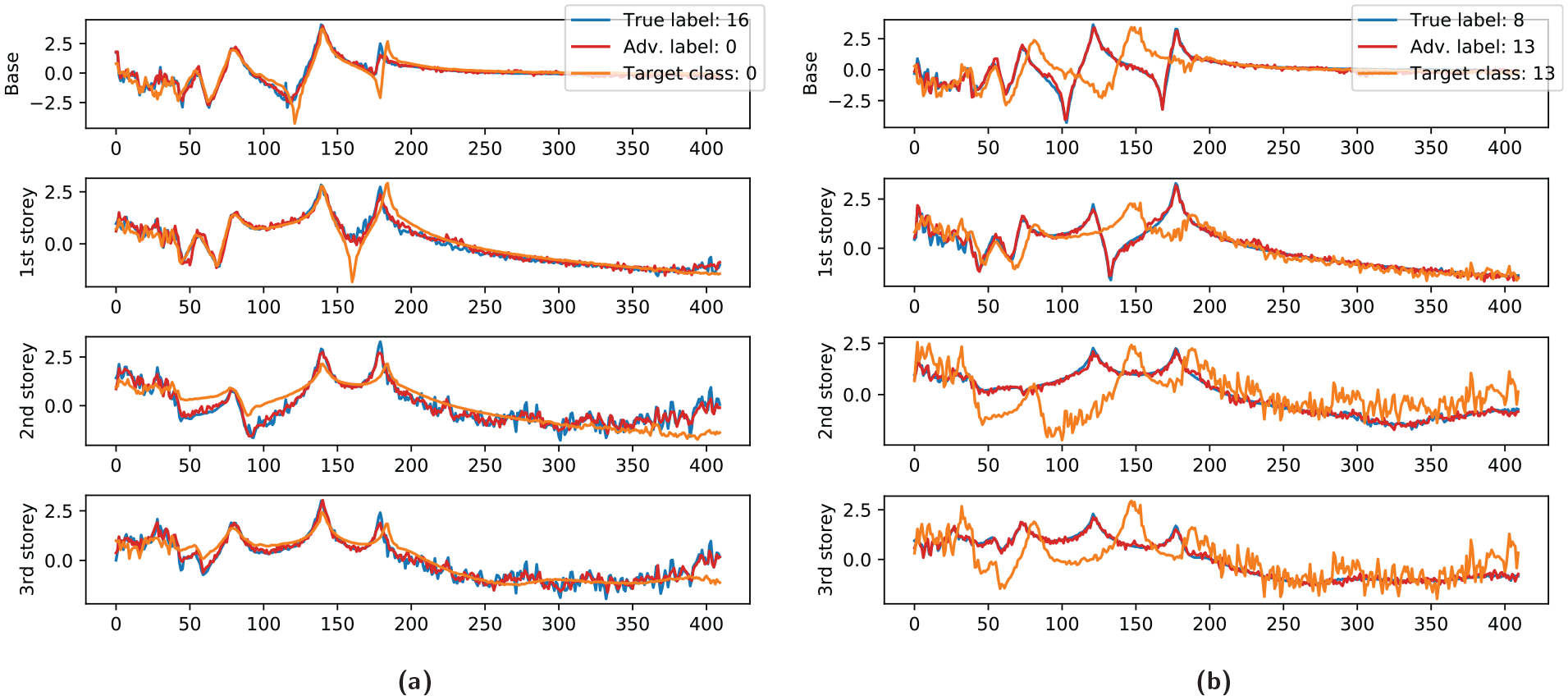
Adversarial examples arising from the white-box attack. The adversarial input is semantically similar and follows the overall structure of the true inputs more closely than the adversarial target signal. There is however a notable difference in the variance of the signal in the false-negative case: (a) false-negative example and (b) false-positive example.
For intuition as to how the semantic structure of the signals remains intact during the perturbation, the first two principal component analysis (PCA) directions of the FRF data are plotted in Figure 10. Overlayed on the figure are 10 of the transformations from true inputs (dots) to adverse examples (crosses) coloured by damage label. In the figure, it can be seen that the perturbation is small in the PCA basis suggesting that the majority of the structure has been maintained.
First two PCA directions of training and validation data (coloured by damage label) as well as latent representation of adversarial perturbation. Arrows show mapping from true examples (dots) to adversarial examples (crosses).
Demonstration of black-box attack
For the black-box attack demonstration, it is assumed that the attacker only has access to the classifier on an input–output basis and has no knowledge of the inner workings of the algorithm. We permit the attacker access to a set of training examples and corresponding target labels, but crucially not the gradient information. While many black-box approaches to adversarial attack rely on the construction of a surrogate model in order to generate a synthetic classifier that can be attacked as a white-box, the approach utilised here is deliberately more naive. It is the reasoning of the authors that vulnerability to such naive attacks lowers the bar for adversarial attack and further motivates investigation into the ways in which SHM algorithms might be made more robust.
The aforementioned approach consists of two phases. During the listening phase a 1024-512-n deep auto-encoder (DAE)
33
is trained to learn a reduced-order representation of the inputs. While other more sophisticated reduced-order models (such as hierarchical models or modal analysis–based approaches) are clearly appropriate, the objective here is to demonstrate a naive approach that makes little to no assumptions about the structure of the input. The DAE consists of two components, the encoding transformation
where
Several authors have studied adversarial attacks on DAEs and other latent space models.34,35 The approach shown here is most similar to that of Creswell et al.
36
in that the latent space is perturbed directly. However, while the authors specify an additive transformation for
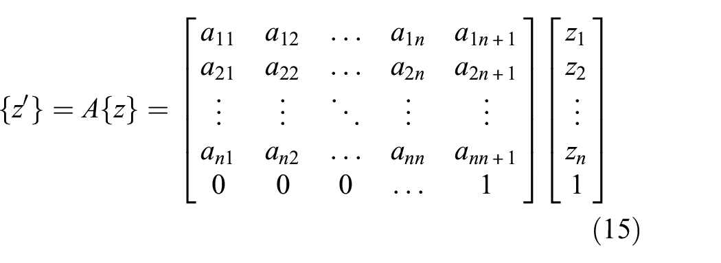
During the learning phase, the DAE is prepended to the classifier and the perturbing transformation is inserted between the encoder and the decoder. The forward adversarial transformation is now given by

As before, this is a multi-objective optimisation problem that seeks to maximise both semantic similarity and miss-classification. The learning phase objective function is now given by
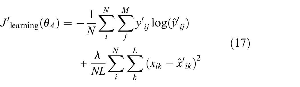
where
The size of the latent encoding represents a trade-off between accurate reconstruction of the inputs and the complexity (number of parameters) of the affine transformation. More parameters in the latent encoding will result in higher fidelity representations of the inputs, but will require more parameters to be optimised in order to find the adversarial transformation. The number of parameters in
In order to select a value for n, the explained variance of the first 50 PCA components are plotted alongside the classification accuracy of the reconstructed signal in Figure 11. Although not directly related, the PCA explained variance plot affords intuition into the number of parameters that are required to provide an accurate representation of the input. It can be seen from the figure that only a small number of parameters are responsible for the majority of the variance in the inputs (this is expected from highly structured data such as FRFs). The classification accuracy does not seem to be affected above values of 5. With this in mind, a conservative value of
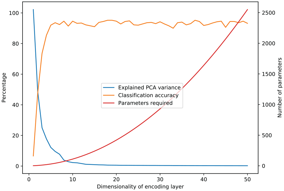
Explained variance of PCA representation, plotted alongside the reconstructed classification accuracy and parameters in the affine transformation for differing values ofn (based on the figure, the value
Figure 12 depicts the input and reconstruction for the trained DAE. It can be seen in the figure that the DAE has done a good job of representing the overall structure of the data but struggles to emulate the variance seen in the higher frequencies of the damaged examples. Nevertheless, this representation is clearly able to capture the damage-sensitive nature of the FRFs as the classification confusion matrix in Figure 13 is largely unchanged.
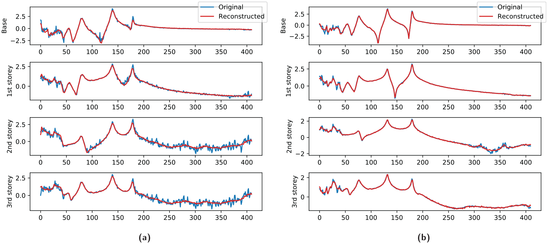
Original inputs and DAE reconstructions after the learning phase. The DAE has learned to represent the structureof the data well but is struggling to reproduce the increased variance in the higher frequencies found in the damaged signals:(a) damaged case and (b) undamaged case.
Confusion matrix of the classifier predictions on the DAE reconstructed signal before adversarial perturbation.
The parameters of the adversarial transformation
Hyperparameters of SADE optimiser.
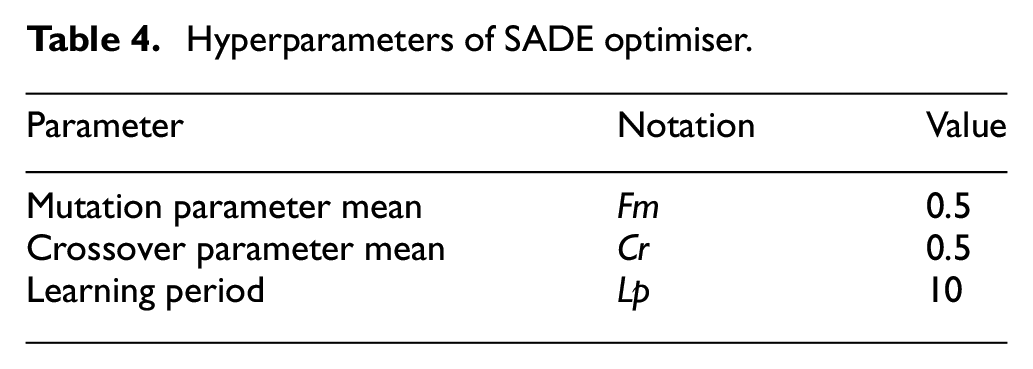
The parameters of 100 trial transformations are optimised over 10 runs from an initial uniform distribution on the interval
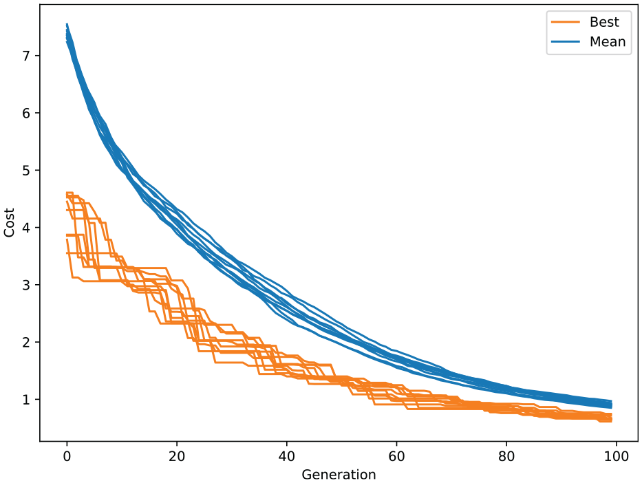
Convergence history of the SADE optimiser over 10 runs.
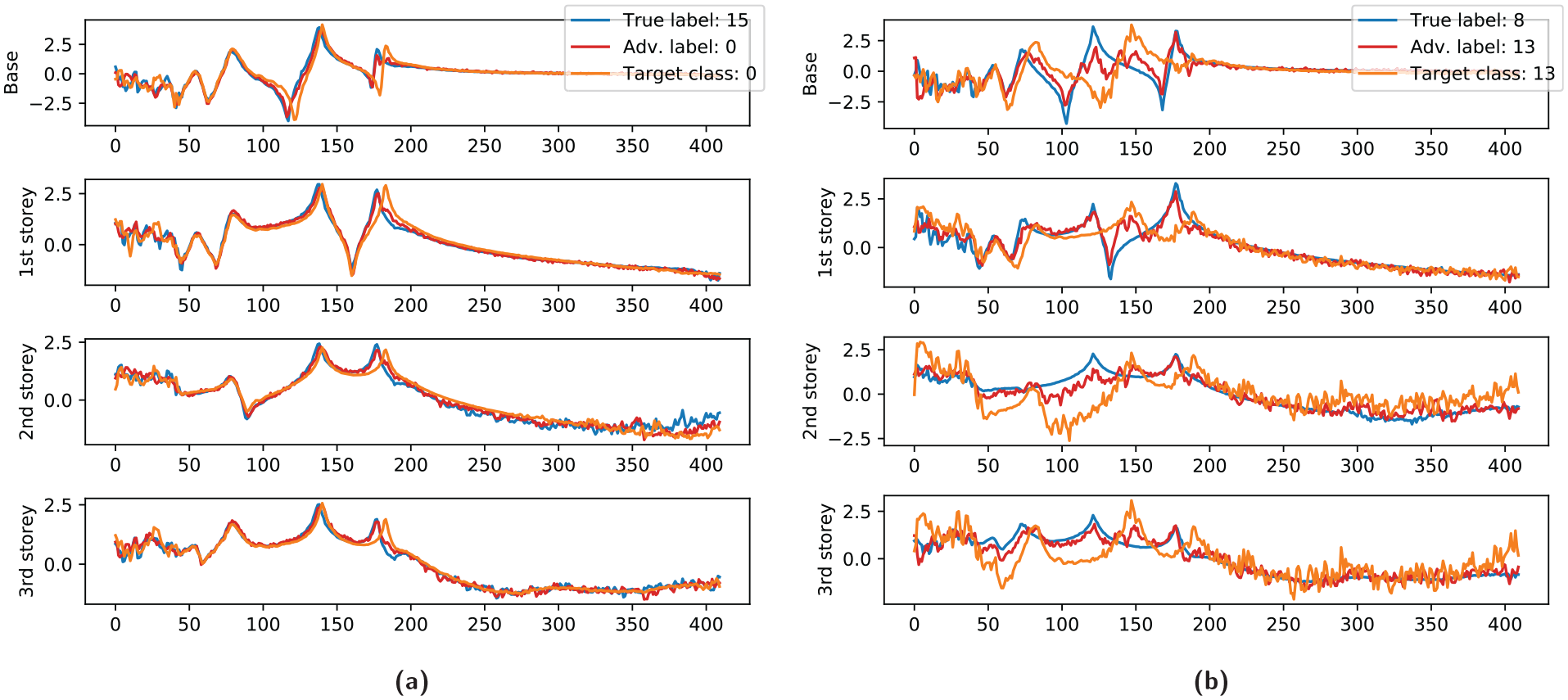
Figure 15 depicts the classification confusion matrix on the unseen data. Although not as successful as the white-box attack, the latent space perturbation has still managed to induce false-positive and false-negative classifications in almost every case. Figure 16 depicts the adversarial examples generated in the black-box attack from the same unperturbed inputs used to generate the examples in Figure 9. However, it is immediately obvious that the black-box attack has failed to produce adversarial examples that maintain semantic similarity to the true inputs. The overall structure of the input has been conserved during the attack and the signals still clearly resemble FRFs. However, the adversarial examples more closely resemble members of the target class, meaning that the chances of such examples fooling a human observer is low.
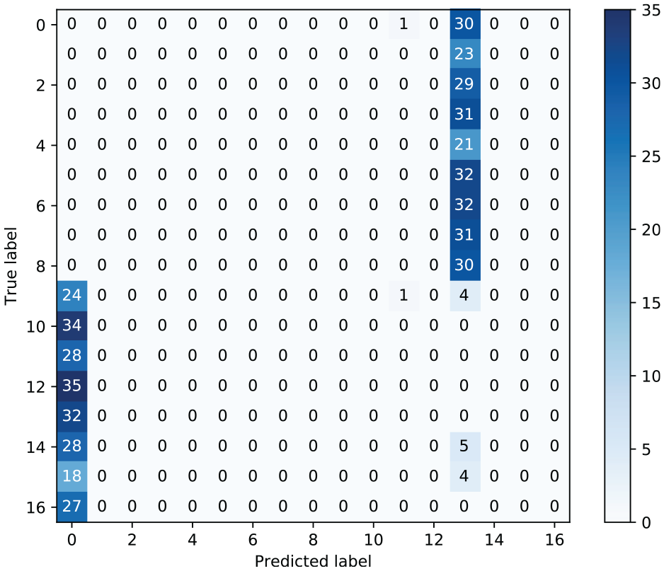
Classification confusion matrix resulting from the black-box attack.
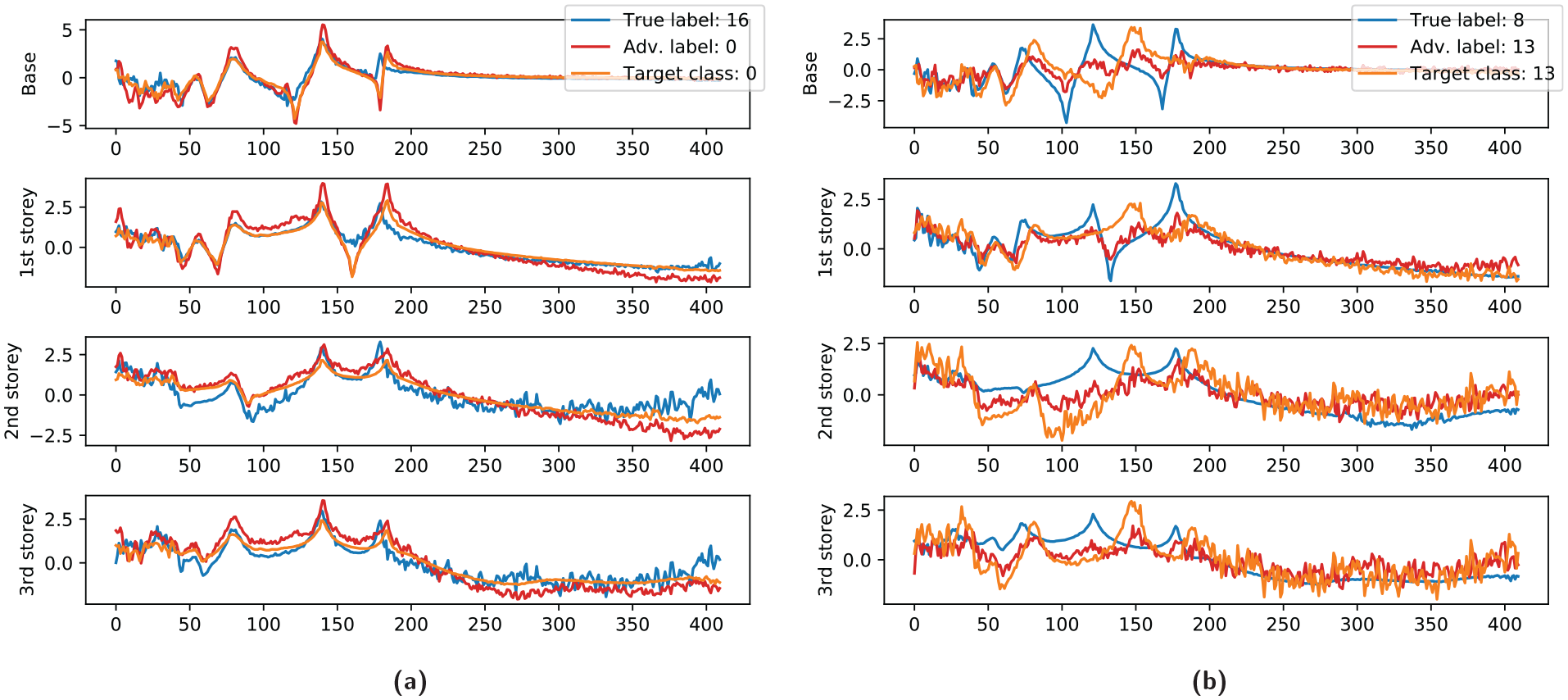
Adversarial examples results arising from a black-box attack. The adversarial examples (red) are semantically more similar to the target class (orange) than the true input (blue): (a) false-negative example and (b) false-positive example.
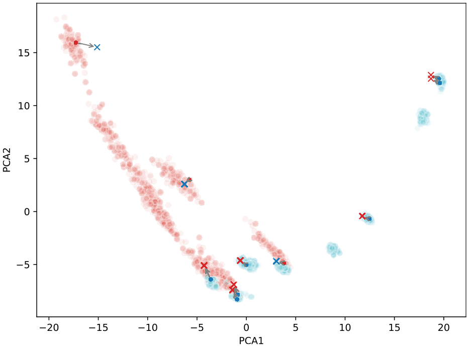
Figure 17 depicts the PCA directions of the dataset for the first 10 adversarial transformations as in Figure 10. In this figure, the reason for the loss of semantic similarity might be explained. The perturbations in the latent space have translated to large shifts in the PCA projection, suggesting that the adversarial examples are structurally quite dissimilar to the true inputs from which they were constructed. Another possible explanation is a poor correlation between latent and classification spaces. The nonlinearity introduced by the decoding layer of the DAE has the effect of exaggerating small changes made in the latent space into large changes in the adversarial examples. Such an effect would make optimisation on the parameters of
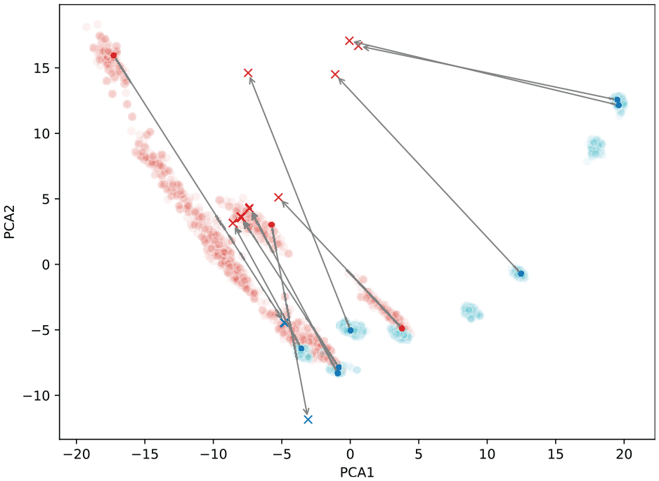
First two PCA directions of training and validation data (coloured by damage label) as well as latent representation of adversarial perturbation (arrow from true to adversarial).
Despite these results, some semantically convincing examples can still be constructed by a variant of the latent attack method described earlier. By optimising the parameters of
Adversarial examples results arising from the second black-box attack, selected for presentation based on a visual assessment of semantic similarity. The adversarial input is semantically similar and follows the overall structure of the true inputs more closely than the adversarial target signal: (a) false-negative example with λ = 80 and (b) false-positive example with λ = 40.
Although these examples were cherry-picked from a large group of potential examples as visually more threatening, the authors would point out that an attacker would also be free to make such a selection. In fact, query limitation would be the only thing preventing an attacker from generating many thousands of trial examples and selecting only the most potent for malicious deployment. In an SHM context, whereby even a small number of false positives (and an even smaller number of false negatives) are enough to render a framework useless, an approach of this type represents a serious threat.
Adversarial defence strategies for SHM
Several adversarial defence strategies have already been presented in the machine learning literature and the development of new approaches is a very active area of research. The development of the techniques has thus far been centred largely around image classification tasks and have often been presented in an ad hoc manner, whereby any one strategy is only effective against a subset of attack types and vise versa.
Of the defences thus far presented, two prominent themes are distillation 38 and adversarial training21,39 type defences. While distillation has been shown to be effective against some common attacks, it has also been shown to be insecure against attacks deliberately designed to circumvent the method. 40 Adversarial training defences generate adversarial examples during the model training process, with the hope that the trained model will develop robustly. While promising progress has been made, the application of this technique in an SHM context is likely to be limited by the availability of damaged training data.
Recently, Ilyas et al. 41 have presented a new approach related to adversarial training based on the theory that adversarial examples arise due to ‘non-robust features’ that are present in the dataset. Their approach utilises a penalty term in the objective function that punishes models that rely on the non-robust features.
Another promising direction is the investigation into generative models. Li et al. 42 have recently suggested that generative models may be more robust to adversarial attacks. They present adversarial defence strategies that are able to make use of the full joint distribution in order to detect adverse examples. This is a promising result for SHM, as many modern approaches utilise models of this type, for example, Bayesian networks. 43 However, Gilmer et al. 44 have shown that the presence of adversarial examples in high-dimensional datasets is (at least in a simplified spherical case) independent of the model used for classification.
Conclusion
In this work, it has been possible to demonstrate the serious vulnerability of an SHM classifier to adversarial attack. A universal example search, has been shown to construct semantically convincing adversarial examples that are able to fool an SHM classifier with almost perfect testing accuracy. This was achieved in the white-box threat scenario, which is the more realistic for SHM applications. Although failing to replicate this feat, a naive black-box attack has also been able to construct individual adversarial examples.
Clearly, robustness to adversarial attack is an open problem that presents a real challenge to the robustness of machine learning applications. This work demonstrates that data-driven SHM methods are not exempted. In order to facilitate further investigation, an adversarial attack threat model for SHM has been proposed. It is hoped that this will serve as a platform for future discussion surrounding the security implications of data-driven SHM approaches. The authors believe that adversarial attack robustness will emerge as a key challenge in the widespread deployment of SHM frameworks.
Footnotes
Funding
The author(s) disclosed receipt of the following financial support for the research, authorship and/or publication of this article: M.D.C. would like to recognise support from EPSRC (grant no. EP/L016257/1). The research presented in this paper was partially supported by the Laboratory Directed Research and Development Programme of Los Alamos National Laboratory under the Information Science and Technology Institute as part of the 2019 Adversarial Machine Learning Challenge.This work was supported in part by the US Department of Energy through the Los Alamos National Laboratory. Los Alamos National Laboratory is operated by Triad National Security, LLC, for the National Nuclear Security Administration of US Department of Energy (contract no. 89233218CNA000001). This study was also financed in part by the Coordenacao de Aperfeicoamento de Pessoal de Nivel Superior – Brasil (CAPES; Finance code 88881. 190499/2018-01).