Sage Journals: Discover world-class research

Abstract

In recent years, the Internet of Things has been widely used in modern life. Advanced persistent threats are long-term network attacks on specific targets with attackers using advanced attack methods. The Internet of Things targets have also been threatened by advanced persistent threats with the widespread application of Internet of Things. The Internet of Things device such as sensors is weaker than host in security. In the field of advanced persistent threat detection, most works used machine learning methods whether host-based detection or network-based detection. However, models using machine learning methods lack robustness because it can be attacked easily by adversarial examples. In this article, we summarize the characteristics of advanced persistent threats traffic and propose the algorithm to make adversarial examples for the advanced persistent threat detection model. We first train advanced persistent threat detection models using different machine learning methods, among which the highest F1-score is 0.9791. Then, we use the algorithm proposed to grey-box attack one of models and the detection success rate of the model drop from 98.52% to 1.47%. We prove that advanced persistent threats adversarial examples are transitive and we successfully black-box attack other models according to this. The detection success rate of the attacked model with the best attacked effect dropped from 98.66% to 0.13%.

Keywords

Internet of Things advanced persistent threats machine learning adversarial examples adversarial attacks

Introduction

Advanced persistent threats (APTs) are long-term network attacks on specific targets with attackers using advanced attack methods. APTs are more advanced than other forms of attacks. APT is advanced because it uses advanced attack tools and methods. Before an APT attack, the attacker will collect as accurately as possible the business process and target system of the attacked object. In addition, APT attacks are far more difficult to detect than traditional non-targeted attacks because APT attacks are targeted, highly concealed, exploit vulnerabilities and do not aim at directly obtaining economic benefits.¹ At first, APT attackers mainly attacked the state and government departments. In recent years, they have begun to attack the private and corporate sectors.² APT attackers also have turned their attack targets from traditional targets to Internet of Things (IoT) targets. IoT threats continued at a rapid pace and APT attackers successfully used timeworn strategies to gain access to vulnerable connected devices.³ As exposed by Drovorub, APT28 hacked IoT devices such as the video decoder and the printer.⁴ Therefore, how to detect and respond to APT attacks has become increasingly important for the cyber security and the IoT security.

The existing APT detection methods are divided into host-based detection methods and network-based detection methods. The host-based detection methods are mainly to detect whether there are malicious behaviours on independent hosts such as the execution of malicious software, the behaviour of applications trying to modify certain files. Bian et al.⁵ extracted graph-based features from authentication logs of the target host during the APT lateral movement stage and then used these features to train the machine learning model to detect APT. Bai et al.⁶ used machine learning methods to detect abnormal behaviours of Remote Desktop Protocol (RDP) event logs during the APT lateral movement stage to detect APT. Yan et al. proposed an AUID framework, which extracts three major categories of features: host-based features, domain-based features and time-based features. Then it uses the K-means algorithm to detect APT.⁷ Ghafir et al.⁸ proposed an APT detection system based on learning, MLAPT, which mainly uses threat detection module, alert correlation module and attack prediction module to detect APT. The network-based detection methods usually take network flow data as input and aim to find abnormal network packets and abnormal network interactions through statistical analysis, data mining or machine learning.⁹ Zhao et al.¹⁰ deployed at the network exit point to extract domain name system (DNS)-related features, then performed APT detection based on signature, abnormal behaviour and the features extracted. Niu et al.¹¹ extracted DNS-related features from the phone’s DNS logs to detect APT. Schindler¹² used the graph method and mapped the time series to the kill chain model through a multi-layer structure, then used machine learning methods to detect abnormal behaviours by learning normal behaviours.

Both host-based detection methods and network-based detection methods have adopted machine learning methods mostly. However, machine learning lacks robustness because it is easily attacked by adversarial examples. The adversarial example is to add some small but intentional perturbations to the input sample, but it can cause the machine learning model to output a wrong classification with high confidence. Previous studies believed that adversarial examples work because of the high non-linearity and over-fitting of the machine learning model; Goodfellow et al. first proposed that the appearance of adversarial examples work precisely due to the machine learning model’s high latitude and high linearization. Relying on this assumption, Goodfellow et al.¹³ proposed the fast gradient sign method (FGSM) to generate adversarial examples and obtained a panda image with a 99.3% confidence of ‘gibbons’. Kurakin et al.¹⁴ used the FGSM and the iterative FGSM (I-FGSM) to generate adversarial examples of images, then use the printed adversarial examples as the input sample and found that it can also mislead the machine learning model. The algorithms mentioned in the previous articles are all white-box attacks, that is, the attacker needs to know the structure and parameters of the attacked model. The following articles are all black-box attacks. Zhou et al.¹⁵ trained an alternative model of the attacked model and then generated adversarial examples against the alternative model to achieve adversarial attacks against the model. Xia et al. used the generative adversarial network (GAN) to alternatively train two neural networks, the generator and the discriminator, the discriminator is used for image classification and the generator is used to generate adversarial examples. Finally, a neural network that can generate adversarial examples is obtained.¹⁶ In the field of detecting malware, Grosse et al.¹⁷ successfully misled the malware detection model by modifying the adversarial examples crafting algorithm for image classification. Hu and Tan¹⁸ used GAN to carry out the black-box attack on the malware detection system and successfully bypassed the system.

It is popular to use machine learning methods to detect APT, but machine learning has proven to be vulnerable to adversarial attacks in many fields. Although it has not been proven that APT detection systems based on machine learning are vulnerable to be attacked by adversarial example, we believe that adversarial attacks against the APT detection model would have occurred or will occur in the future because the nature of machine learning methods are vulnerable to adversarial attacks. And because APT attacks are more advanced in attack tools and methods than other network attacks, APT attackers are likely to use the characteristics of machine learning models to mislead or even paralyse our APT detection models based on machine learning methods.

To verify that machine learning methods used in the APT field are also vulnerable to attacks from adversarial examples, this article first extracts network-based features from the acquired network flow data and trains APT detection models through these features to detect APT attacks by detecting abnormal networks. Then we use the algorithm proposed to grey-box attack and black-box attack APT detection models.

In summary, we make the following contributions.

We train APT detection models based on network traffic features and prove that the model can detect APT attacks effectively.

We summarize the characteristics of APT traffic and propose the adversarial examples generation algorithm in the field of APT based on these characteristics. Then, we use this algorithm to grey-box attack APT detection models.

We prove that the emergence of APT adversarial examples is due to the high linearity of machine learning model. In addition, we also prove that APT adversarial examples are transitive and use this characteristic to black-box attack APT detection models.

Related work

APT

The life cycle of APT can be divided into the following stages: reconnaissance, delivery, initial intrusion, command and control (C&C), lateral movement, data exfiltration.¹⁹ In the reconnaissance and delivery stage, attackers mainly collect information about the target, such as exploits, personnel information and host information. Then attackers use collected information to attack the target in the initial intrusion stage. In the C&C stage, attackers use the C&C server to control compromised hosts. In the lateral movement stage, attackers go through compromised hosts to move inside network and expand control. In this stage, attackers can control new compromised hosts and these hosts can also be used to infect more hosts of inside network. Finally, attackers can steal sensitive data from the target. Compared with traditional cyber intrusions, APT has the following characteristics: (a) advanced – attackers use advanced attack tools and methods, 0 day vulnerabilities are often used in APT attacks, but traditional attacks are rarely used; (b) targeted – attackers have clear targets and collect information about the target from the beginning, but traditional cyber-attacks often have no clear targets; (c) highly concealed – attackers will stay as concealed as possible in the host to obtain confidential information for a long time,¹ APT attackers often stay in the host for hundreds of days. Due to these characteristics, APTs are difficult to be detected by traditional detection techniques, such as intrusion detection technology, vulnerability detection technology and malicious code detection technology.²⁰

IoT have been widely used in modern life. IoT refer to the system composed of interconnected and interrelated devices, objects and sensors.²¹ IoT targets have also been threatened by APTs with the widespread application of IoT because the IoT device such as the sensors is weaker than host in security. How to detect and respond to APT attacks has become increasingly important for the IoT security since IoT devices are inherently risky and easy to exploit while being heavily exposed to the Internet.²²

As exposed by Drovorub, APT28 hacked at least 500,000 IoT devices, such as routers, video decoders and printers.⁴ APT28 attackers usually use phishing emails to carry out attacks and then use botnets to control IoT devices. In an intrusion activity, APT28 attackers invaded three IoT devices: video decoders, VOIP phones and printers. In the initial intrusion stage and the C&C stage, attackers took control of the printer by exploiting the vulnerability and controlled the video decoder and the VOIP phone by using the default password. In the lateral movement stage, attackers used compromised IoT devices to perform intranet penetration. In addition, attackers can steal sensitive data from the target in the end.

Adversarial attacks

Machine learning has a wide range of applications in many fields. Akinyelu and Adewumi²³ used the random forest method to propose a content-based phishing detection model, which can detect extremely harmful phishing emails from normal emails. Girshick et al. combined the region proposal with convolutional neural networks (CNNs) to propose R-CNN, which achieved target detection. This method first extracted about 2000 bottom-up regional suggestions from the input image, then used CNN to calculate the feature value of each suggestion. Finally, the support vector machine (SVM) method used the extracted feature values to classify each region.²⁴ As the number of layers of a neural network increases, its error rate will also increase. To solve this problem, He et al.²⁵ proposed a residual learning framework based on deep convolutional neural networks and improved the classification accuracy on the ImageNet dataset. Simonyan and Zisserman²⁶ proposed that a convolutional neural network with deep layers can be used to classify images with a large classification range. Machine learning classifiers have also been widely used to detect malware. The effectiveness of malware detectors will decrease as malware evolves, Nataraj et al.²⁷ innovatively mapped the malware binary byte file into a gray-scale image and then detected the malware through image classification methods. Raff et al.²⁸ proposed a malware detection model based on convolutional neural networks, which mainly used neural networks to test the binary code of the entire file. Alsulami et al. proposed a neural network model based on convolution and long short-term memory (LSTM) to detect the behaviour of software. This model extracted features from Windows pre-reading files to realize malware detection.²⁹

With the widespread application of machine learning in various fields, the security issues of machine learning cannot be underestimated. The methods of attacking machine learning are mainly divided into attacks in the training phase and attacks in the inference phase. Poison attacks are mainly polluting the training set in the training phase of the machine learning model. Shike Mei and Zhu³⁰ successfully poison attacked the logistic regression model, the linear regression model and SVMs through the optimized training set attack. Adversarial attacks are mainly constructing adversarial examples in the inference stage of the machine learning model. Adversarial examples are generated by performing small disturbances on the input samples according to a specific algorithm. However, the machine learning model’s classification of the original input example and the adversarial example are different, it can be formulized as Equation (1)

F (x) \neq F (\bar{x})

(1)

where $F$ represents our APT detection models, $x$ represents the original input example, $\bar{x}$ represents the adversarial example obtained by modifying $x$ .

The process of misleading the model by generating adversarial examples is called an adversarial attack. The main problem of adversarial attacks is how to modify the original example to obtain the adversarial example. Adversarial attacks can be divided into white-box attacks and black-box attacks according to the attacker’s knowledge of the machine learning model. The attacker of white-box attacks not only knows the structure adopted by the attacked model, but also knows parameters of the model.^13,14,17 The FGSM is a typical white-box attack algorithm. FGSM obtains the gradient of the current input example for the model and then modifies the input example according to the gradient to obtain the adversarial example. Goodfellow et al.¹³ used FGSM to generate adversarial examples for image classification. Grosse et al. used FGSM to generate adversarial examples against malware classification.¹⁷ Kurakin et al.¹⁴ proposed I-FGSM, an iterative version of FGSM based on FGSM. The attacker of black-box attacks only knows the classification of the current input example for the attacked model.^15,16,18,31 Zhou et al. adversarial attacked the machine learning model without using real data, which obtained uniformly distributed synthetic data through the generative model. Zhou et al.¹⁵ trained an alternative model through the classification result of the attacked model on synthetic data and then white-box attacked the alternative model to complete adversarial black-box attacks. GAN can also be used to generate adversarial examples. GAN used the generative model to generate adversarial examples and used the discriminative model to classify adversarial examples and benign input examples. Xia and Liu¹⁶ used GAN for adversarial attack on the image classification model. Hu and Tan¹⁸ used GAN for adversarial attack on the malware detection model. Su et al.³¹ achieved adversarial attacks by randomly modifying a pixel of the input image based on differential evolution.

Methodology

Dataset

The APT detection model generated in this article based on network and the model detects abnormal network-related information through statistical analysis of network data streams to detect APT.

The benign traffic used for training the APT detection model comes from TcprePlay, which is real network traffic captured on busy private network access points. The size of normal traffic is 368 MB including 40,686 network stream data and 791,615 data packets generated by 132 applications.³²

The APT traffic used for APT detection model is the real APT example that comes from Contagio malware database, which contains 5732 data packets.³³ The same APT traffic is used by many related works.^34,35 The APT traffic includes 36 datasets consisting of 29 APT samples. In our dataset, the APT traffic accounts for about 1% of the normal traffic, which is consistent with that in real life. The low proportion makes it difficult to detect APT.

Training the APT detection model

There are six steps in the process of training the APT detection model, which is shown in Figure 1. In the following sections, we will introduce every step on how to test the model.

Figure 1.

The process of training the APT detection model. This process consists of six steps. APT: advanced persistent threat.

Raw data analysis

In the raw data analysis stage, we first used Wireshark to analyse the pcap file of the original raw data. The pcap file in the data set is the network packet and Wireshark are very popular network analysis software. Wireshark can intercept many kinds of network packets and it can also display the detailed information of the network packet obtained, such as source IP address, destination IP address, length and the protocol. In this section, we use Wireshark to obtain detailed information of the original data, which can make preparation for subsequent statistics and feature extraction.

Statistics and feature extraction

At the step of statistics and feature extraction, we use the scapy program to perform statistics and feature extraction on the original data based on the results of the previous analysis. The scapy program is a very powerful network data packet processing tool. It can forge data packets, decode data packets, capture data packets and send data packets through the network.

The selection of extracted features is not only based on the previous analysis of the original data, but also based on the analysis of the existing network-based APT detection literature.^10,28,34,36 Features we propose are divided into data stream-level features and packet-level features. The features extracted in this article for detecting APT are as follows.

Source port and destination port: To pass the firewall, APT attackers will use the C&C communication protocol and port allowed by the firewall.¹⁰ By analysing the traffic, we found that destination ports used by APT traffic are mostly popular port such as 80, while ports used by normal traffic are mostly dynamic.

Protocol: There may be a mismatch between the port and the protocol, because the protocol used by APT attackers is implemented at the encoding stage and the port is configured when locating the C&C server.¹⁰

The duration of stream: By comparing and analysing normal traffic and APT traffic, we found that the network flow duration of APT traffic is almost all greater than 0.1 s (99.3%), while the network flow duration of normal traffic is mostly less than 0.1 s (64.9%). The reason why the flow duration of APT traffic is greater than normal traffic is because APT traffic needs to take time to evade the defence system.

The number of data packets and traffic bits: To hide themselves, APT attackers will generate fewer packets and bits than normal traffic.²⁸

The number of bits in a data packet: The average packet size of APT traffic is much smaller than normal traffic,³⁴ because the goal of normal traffic is to transmit information and other normal behaviours, while APT traffic is to invade the system.

The number of data packets per unit time: To remain concealed and maintain interaction with the attacked system, APT attackers will generate a small amount of data packets for a long time.³⁶ However, normal traffic will transmit a large number of data packets in a short period of time.

The time interval of upstream data packets: There is almost no time interval between upstream data packets in normal traffic, while there is time interval between upstream data packets of APT traffic.³⁴

The time interval of downstream data packets: Due to the time interval between the upstream data packets in APT traffic, there is also a time interval between the downstream data packets. It also will be slightly larger than the time interval of the upstream data packets in APT traffic.³⁴

The ratio of upstream to downstream: In normal traffic, the host upload traffic to the network is greater than the download traffic from the network. In APT traffic, the infected host will send host information to the attacker for further attacks instructions, so the upstream traffic will be larger than the downstream traffic.¹⁰

The ratio of upstream data packets to downstream data packets: In APT traffic, the upstream data packet will be significantly larger than the downstream data packet.³⁴

Stream bits per unit time: The APT attacker will keep low traffic through the firewall, so the stream bit per unit time of the APT traffic will be less than the normal traffic.³⁴ Comparing and analysing the normal traffic and the APT traffic can also prove it.

Split dataset

Before splitting the dataset, we need to perform one-hot encoding on the protocol, because it is a categorical variable. We also add the feature of label because the training process of the APT detection model belongs to supervised learning. We mark the APT traffic (positive examples) as 1 and mark the normal traffic (negative examples) as 0. In this step, we divide the dataset into the training set and the testing set. Then we randomly divided the data set into the training set and the test set according to the ratio of 80% and 20%.

Standardization

The effect of model will be affected by different value ranges and dimensions in different features and the existence of singular examples. Therefore, extracted features must be standardized before training the APT detection model. The standardized data will be in the same order of magnitude, that is, have the same value range. The standardized process is as shown in Equation (2)

x^{*} = \frac{x - μ}{σ}

(2)

where $x$ represents the data before standardization and $x^{*}$ means the standardized data, $μ$ and $σ$ are the average and standard deviation of the training set of the current feature, respectively. After standardization, the average value of feature is 0 and the standard deviation is 1. It is worth noting that before using the test set, it should also be standardized with same parameters.

Training the classifier model

After standardization, we train four different APT detection models based on different machine learning algorithms. The data set used to train our models is the training set previously divided in the split dataset step. These models can successfully detect APT traffic from normal traffic. We select the k-nearest neighbour (KNN) algorithm, the random forest algorithm, the logistic regression algorithm and the SVM as the algorithm for training our models. The model we selected includes linear models and non-linear models, which can measure the adversarial example generation algorithm comprehensively. The algorithms we choose to train our model are based on related works.^34,37 According to our evaluation in the section ‘Experimental results and discussion’, these models are able to detect APT very effectively.

Testing the APT detection model

This step is used to test whether our model can detect the APT traffic. The data set used to test our models is the testing set previously divided in the split dataset step. The training set occupies 80% of the data set and the test set occupies 20% of the data set. To train our model and reach a better training effect, the training set is greater than the testing set. Before we test the model, we should standardize the testing set. When the training set is standardized, the training set does not need to recalculate its own $μ$ and $σ$ value. It should be standardized with same parameters, which the training set used. Although we randomly divide the data set, we use the same divided test set for different models when testing the model and the same training set is used when training the model. Test indexes and test results are shown in the section ‘Experimental results and discussion’.

Crafting adversarial examples

In this section, we will focus on the adversarial example generation algorithm in the field of APT attack detection. According to the adversarial sample generation algorithm, attackers can fool the APT detection model through simple calculations. The process of using adversarial example generation algorithm to generate adversarial examples is called adversarial attacks. Adversarial attacks are mainly divided into white-box attacks and black-box attacks. In addition, the algorithm we proposed are grey-box attacks. This means that even if attackers have limited information about the target, they can also have adversarial attacks on the target model.

Both white-box attacks and black-box attacks are designed to mislead the APT detection model so that it cannot detect the APT traffic from the normal traffic. White- box attack means that the attacker fully understands the internal structure and the training parameters of the model.^13,14,17 Black-box attack means that the attacker only knows the model’s corresponding classification results for input examples.^15,16,18,31 In real life, the attacker can neither fully understand the model nor be ignorant of the model. Moreover, the adversarial attack in this article is the grey-box attack, between the black-box attack and the white-box attack. Grey-box attack means that the attacker can understand part of the information of the model. In this article, we assume that the attacker knows the output probability of the model for the input example.

Current adversarial attacks are most aimed at the field of computer vision image classification and malware detection. Next, this article will analyse the characteristic of existing adversarial attacks and combine the characteristic of APT traffic to propose the adversarial example generation algorithm in the APT detection field. The Modified National Institute of Standards and Technology (MNIST) dataset is mostly used in the field of image classification.^13,16,38Each picture in MNIST is a gray-scale image composed of 28 times by 8 pixels. The grey value of each pixel is 0–255. In addition, the CIFAR-10 data set is also used.³¹ Each picture in CIFAR-10 is a colour image composed of 32 times 32 pixels. Each pixel in a colour image has three components, R, G and B, and each component ranges from 0 to 255. In the field of image classification, a pixel of the image is a feature. In the field of malware detection, each feature represents a function of the software.¹⁷ Grosse et al. extracted 545,333 features in malware detection. Features extracted are all binary and discrete variables, where 1 means that the software has this function and 0 means that it does not. In addition, the function of a single malware is very limited compared to the entire feature, so the input feature vector of a single malware is very sparse. Grosse only added functions when making adversarial examples because the deletion of functions may affect the offensiveness of malware. In addition, the malware’s adversarial example generation algorithm imposed an L1-norm limit on the number of functions modified, which is limited to less than 20.

We can find that features of input examples are all discrete values whether in the field of image classification or in the field of malware detection. The range of every feature is also consistent. The range of features in the field of image classification are all 0 to 255 and the range in the field of malware detection are all 0 or 1. By comparing and analysing the characteristics of APT input samples and other fields, we can find that APT traffic has the following characteristics:

Attributes of features are different: Features we extract have discrete values such as port, the number of data packets and also have continuous values such as the duration of stream.

Features’ orders of magnitude are different: the order of magnitude between features is different. The duration of stream has −3 orders of magnitude and stream bits per unit time has 3 orders of magnitude, the difference between two features is 6 orders of magnitude. The order of magnitude between different examples in the same feature is also different. These determine that there is no fixed range of modification when generating adversarial examples.

The number of features is small: There are at least 784 features in the field of image classification and 545,333 in the field of malware detection. However, we extracted only 13 features and this determines that the degree of modification when we generate adversarial examples will be slightly greater than the other two fields.

Before proposing the algorithm for generating adversarial examples, we first explain its principle. The training process of the machine learning model is to find an optimal model parameter $θ$ , where $θ$ is satisfied to minimize the loss function of the input example. The process can be formulized as shown in Equation (3)

θ = argmin \frac{1}{2 m} \sum_{i = 1}^{m} {(h_{θ} (x^{(i)}) - y^{(i)})}^{2}

(3)

where $m$ represents the number of input examples, $h_{θ} (x^{(i)})$ represents the probability that the model predicts of the ith input example is positive, $y^{(i)}$ represents the actual label value of the input example.

In short, the training process of the machine learning model is to continuously adjust the model parameters $θ$ without changing the input example to find a solution that can minimize the loss function of the input example. The algorithm for generating adversarial examples is just the opposite. The algorithm is based on the model that has been trained, that is, the model parameters $θ$ are determined. The algorithm increases the loss function by appropriately modifying the input examples. It is as shown in Equation (4)

\bar{x} = argmax {(h_{θ} (\bar{x}) - y)}^{2}

(4)

where $\bar{x}$ represents the adversarial example obtained after the adversarial example generation algorithm is performed on the current input sample $x$ , $h_{θ} (\bar{x})$ represents the probability that the model predicts of the current adversarial example is positive, $y$ represents the actual label value of the current example. The generated adversarial example $\bar{x}$ should satisfy that the model’s prediction of the adversarial example $h_{θ} (\bar{x})$ does not match the actual value $y$ as much as possible.

Few people will disguise the normal traffic as the APT traffic when considering that in actual situations, so the adversarial example generation algorithm proposed will be only for the traffic, that is, the APT traffic will be disguised as the normal traffic. Combining the characteristics of APT traffic, we propose the adversarial example generation algorithm as shown in Algorithm 1.

Algorithm 1.

Crafting adversarial examples for APT detection model.

Input: α, X, F
1: forx in Xdo
2: forx_i in x do
3: ifF(x_i)>(1−F(x_i) then
4:

δ \leftarrow α \times x_{i}

x_{i} \leftarrow argmin (F (x_{i}), F (x_{i}) + δ, F (x_{i}) - δ)

6: end if
7: end for
8: returnx
9: end for

Our algorithm is based on the linearity of the attacked model.¹³ Small disturbances will gather together to successfully attack the model. In the process of generating adversarial examples, we should modify every feature that can be modified as much as possible because the number of features we extract is less than that other literature.^13,16,17,29 We do not modify protocol, port and other features because these features may become floating point values after our algorithm is modified, which does not match the actual situation. As mentioned earlier, the feature’s order of magnitude is different. If we use the same amount of modification for each feature, the modification is likely to be insignificant for one feature while completely covering the original value for another feature. In addition, we will calculate the modification amount according to a certain proportion of the original value before we modify the feature. This process is indicated in the fourth line of the algorithm where $x_{i}$ is the original value and $δ$ is the modification; we will discuss the different values of $α$ later. In the previous description, we assumed that our attack is the grey-box attack, that is, we can obtain the output probability of the model for the input example. $F (x_{i})$ in the algorithm is the probability of the input sample being the positive example when the ith feature of the input example is $x_{i}$ . Since the model is a binary classification model, $1 - F (x_{i})$ is the probability of the input sample being the negative example when the ith feature of the input example is $x_{i}$ . We select the feature perturbation that can minimize the positive example probability of the input sample as shown in line 5 of the algorithm.

Experimental results and discussion

Evaluation indexes

The accuracy rate cannot measure the effect of our algorithm well due to the imbalance between positive examples and negative examples in our dataset. We also use precision, recall and F1-score to measure our algorithm in addition to the accuracy rate. The formula of each index used is as shown in Equations (5)–(8)

accuracy = \frac{TP + TN}{TP + FN + FP + FN}

(5)

precision = \frac{TP}{TP + FP}

(6)

recall = \frac{TP}{TP + FN}

(7)

F 1 - score = \frac{2 \times precision \times recall}{precision + recall}

(8)

where TP represents the number of positive examples recognized as positive examples, TN represents the number of negative examples recognized as negative examples, FP represents the number of negative examples recognized as positive examples, FN represents the number of positive examples recognized as negative examples.

The evaluation of APT detection models

We train four different APT detection models based on the KNN algorithm, the random forest algorithm, the logistic regression algorithm and the SVM algorithm. The learning curve of APT detection models is shown in Figures 2 –5. The abscissa is the size of the training set. The ordinates are the accuracy of the training set and the testing set. From Figures 2 –5, we can see that the accuracy of the testing set increases as the size of training set increases. Eventually, the accuracy of the testing set and the training set is almost the same, which indicates that our models can detect APT effectively.

Figure 2.

The learning curve of the KNN model. KNN: k-nearest neighbour.

Figure 3.

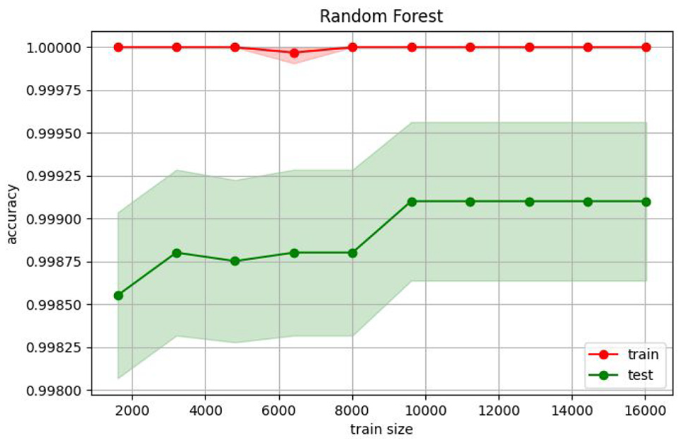
The learning curve of the Random Forest model.

Figure 4.

The learning curve of the Logistic Regression model.

Figure 5.

The learning curve of the SVM model. SVM: support vector machine.

Next, we evaluate the model according to the evaluation index. The experimental results are shown in Table 1. We can see that accuracy rate of the four models we trained are all high, but precision and recall of them are different. From the perspective of F1-score, we can see the model effects of the KNN model, the random forest model and the SVM model are better than the logistic regression model. The random forest model has the highest F1-score, which is 0.9791, followed by the SVM model whose F1-score is 0.9760 and that of the KNN model is 0.9730. The logistic regression model has the lowest F1-score, which is 0.8167. This is because the logistic regression algorithm is too linear to capture the non-linear characteristics in the data well.

Table 1.

The experimental results of APT detection models.

Classifier	Accuracy	Precision	Recall	F1-score
KNN	0.9982	1.0000	0.9474	0.9730
Random Forest	0.9986	1.0000	0.9591	0.9791
Logistic Regression	0.9886	0.9071	0.7427	0.8167
SVM	0.9984	1.0000	0.9532	0.9760
ATCTDS	0.9974	0.9699	0.9415	0.9555

APT: advanced persistent threat; KNN: k-nearest neighbour; SVM: support vector machine; ATCTDS: automated temporal correlation traffic detection system.

To verify the effectiveness of our model for detecting APT attacks, we compare our APT detection models with automated temporal correlation traffic detection system (ATCTDS).³⁴To control the variables, we reproduced the ATCTDS model in the same computing environment with the APT detection models. We choose ATCTDS as the comparison model because ATCTDS utilize the same APT example with us. Moreover, part of the features of the training model used in this article are extracted according to ATCTDS. From Table 1, we can see that ATCTDS is weaker than the KNN model, the random forest model and the SVM model but better than the logistic regression model in precision and recall. This proves that the APT detection model we generated, apart from the logistic regression model, are able to detect APT traffic effectively.

The evaluation of adversarial examples on APT detection models

First, we apply the adversarial example generation algorithm proposed to the APT traffic, that is, the positive example. We do not make adversarial examples for the normal traffic because few people disguise the normal traffic as the APT traffic in reality. Second, we re-select the evaluation index to measure the effect of adversarial examples. We choose the success rate of positive examples classified as positive examples by the APT detection model as the evaluation index. The lower the success rate, the better the effect of the adversarial example generation algorithm’s attack. The formulation of the success rate is as shown in Equation (9)

success rate = \frac{TP}{TP + FN}

(9)

Although the formula for calculating the success rate is the same with the recall, their meaning is completely different. The recall is one of index to evaluate the performance of the APT detection model, but the success rate in this article is used to evaluate the attack effect of the adversarial example generation algorithm. We first generate adversarial examples for the SVM model. The attack effect of adversarial examples for the SVM model is shown in Table 2. The $α$ is the disturbance rate.

Table 2.

The attack effect of adversarial examples for the SVM model.

$α$	Success rate
0	0.9852
0.005	0.9678
0.010	0.9570
0.015	0.9289
0.020	0.8819
0.025	0.7839
0.030	0.6846
0.035	0.1678
0.040	0.0147

SVM: support vector machine.

We limit the disturbance rate $α$ from 0 to 0.040. We do not modify the initial example when $α$ is 0. When the disturbance rate is 0, the success rate is different from recall in Table 1 because the success rate is calculated for all APT examples, but recall is calculated only for the APT examples in the test set. We can see the relationship between the disturbance rate $α$ and the success rate of the APT detection model: the success rate of the model decreases as the disturbance rate increases. In other words, the attack effect of adversarial examples is better as the disturbance increases. This also verifies that the adversarial examples can be successfully generated because of the high linearization of the model.¹³ We apply small perturbations to each feature of the input example and the accumulation of these small perturbations will eventually bias the model’s classification on the input example. We can observe from Table 2 that the success rate of the SVM model decreases from 0.9852 to 0.0147 with $α$ increasing from 0 to 0.040. In other words, the attacking success rate of our proposed method is 0.9853. The decrease in the success rate proves that we successfully adversarial attacked the APT detection model, which also verifies that in the field of APT detection, models using machine learning are vulnerable to attacks from adversarial examples.

Zhou et al.¹⁵ first trained an alternative model of the attacked model and then successfully adversarial attacked the model by generating adversarial examples for the alternative model. Different models may learn similar features and decision boundary for the same input example, so the adversarial samples generated in one model may also be offensive for another model. In other words, adversarial examples are transitive. According to this, we input adversarial examples generated for the SVM model into the other three models, namely, the KNN model, the random forest model and the logistic regression model. Generating adversarial examples for the SVM model belong to the grey-box adversarial attack because we can acquire the output probability of the SVM model for the input example. Moreover, we input adversarial examples into the KNN model, the random forest model and the logistic regression model belonging to the black-box adversarial attack because we can only acquire the binary output result of the input example. The experimental results of the black-box attack against the other three models are shown in Table 3.

Table 3.

The success rate of the other models for adversarial examples.

$α$	KNN	Random forest	Logistic regression
0	0.9651	0.9892	0.7826
0.005	0.9651	0.9825	0.1101
0.010	0.9651	0.9825	0.0268
0.015	0.9651	0.8939	0.0013
0.020	0.9651	0.8899	0.0013
0.025	0.9651	0.6658	0.0013
0.030	0.9651	0.5584	0.0013
0.035	0.9651	0.4295	0.0013
0.040	0.9651	0.0241	0.0013

KNN: k-nearest neighbour.

From Table 3, we can see that with the increase of the disturbance rate, both the random forest model and the logistic regression model show the decrease in the detection success rate. The success rate of random forest model decreases from 0.9866 to 0.0241 and the success rate of logistic regression model decreases from 0.7826 to 0.0013. The attacking success rate of our algorithm for the random forest model and the logistic regression model is 0.9759 and 0.9987. The logistic regression model is weaker than other models for adversarial examples because the model is very linear. The KNN model does not change in the success rate for adversarial examples with different perturbation rates. This is due to the high non-linearity of the KNN model. The algorithm principle of KNN is that if most of nearest examples of an example in the feature space belong to a certain category, the example also belongs to this category. Therefore, the KNN model will not be affected by minor disturbances. The SVM model, the random forest model and the logistic regression model have different degrees of decline in the success rate for adversarial examples under different disturbance rates or we can say that the greater the perturbation rate, the lower the success rate.

In summary, we can conclude that APT adversarial examples have the following two characteristics. First, the emergence of APT adversarial examples is due to the high linearity of the APT detection model. The attack effect of adversarial examples against non-linear models is worse than against linear models. Second, the APT adversarial example is transitive. That is, when the detailed information of the attacked model cannot be obtained, we can train an alternative model and generating adversarial examples for it, the adversarial example is also work for the attacked model. According to the characteristics, we successfully grey-box and white-box attack the APT detection models with adversarial examples.

Comparative experiment

To further demonstrate that the adversarial example generation algorithm proposed for the APT traffic is effective, we compare our methods with existing adversarial examples generation methods. In the field of APT detection, no algorithm for generating adversarial examples has been proposed in the previous study. We compare our method with the famous FGSM algorithm in the field of image classification.¹³ The attack algorithm of FGSM is as shown in Equation (10)

\bar{x} = x + ϵ \times sign (\nabla_{x} J (x, y))

(10)

where $\bar{x}$ means the adversarial example obtained after the FGSM algorithm is performed on the current input sample $x$ , $s ign (\nabla_{x} J (x, y))$ is the gradient direction of the model for the current input, $ϵ$ means the step size of the perturbance.

The key of FGSM is the value of $ϵ$ . The information of input examples will be covered if the $ϵ$ is too large and the algorithm will not work if the $ϵ$ is too small. By analysing the original data, we can find that most of the values are greater than 0.05 except for few values. We choose 0.005 as the value of $ϵ$ through experiments and data analysis. The difference between FGSM and our method is the value of $ϵ$ . The $ϵ$ of FGSM is fixed, but $ϵ$ of our method is calculated based on the current feature value. The value of the current feature is different for different features and different input examples, so the $ϵ$ is also different. The success rate of FGSM and our method for APT detection models is shown in Table 4.

Table 4.

The success rate of APT detection models for adversarial examples generated by FGSM and our method.

Method	SVM	KNN	Random forest	Logistic regression
Original data	0.9852	0.9651	0.9892	0.7826
FGSM	0.9718	0.9651	0.9879	0.0027
Our method	0.0147	0.9651	0.0241	0.0013

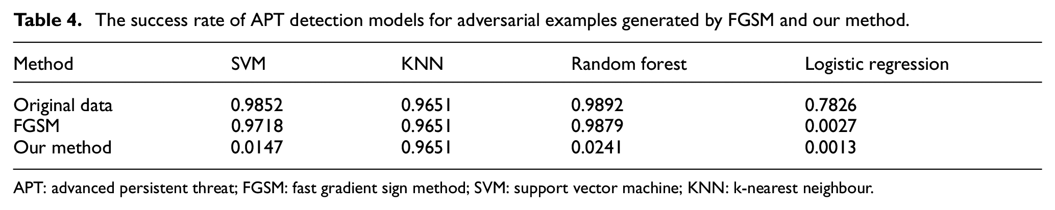
APT: advanced persistent threat; FGSM: fast gradient sign method; SVM: support vector machine; KNN: k-nearest neighbour.

From Table 4, we can see that FGSM only works for the logistic regression model. Both our method and FGSM can successfully attack the logistic regression model due to the high linearity of the logistic regression model. But apart from the logistic regression model, our method also works well for the SVM model and the random forest, but the FGSM does not. To see the comparison more intuitive, we convert Table 4 to Figure 6.

Figure 6.

The comparison of success rate of FGSM and our method. FGSM: fast gradient sign method; SVM: support vector machine; KNN: k-nearest neighbour.

Apart from the KNN model being hardly attacked by adversarial examples due to its high non-linearity, our method works very well than FGSM in generating adversarial examples for the APT detection model as can be seen from Figure 6. And the reason why our method works well is because it is proposed based on the characteristics, whereas FGSM is proposed for image classification.

The results of the above comparative experiments show that our method of generating adversarial examples for the APT detection model is better than the FGSM method. Moreover, our method can successfully attack the APT detection model through adversarial examples with high attacking success rate.

Conclusion

In this article, we notice that the model using machine learning methods is highly linearized through literature reading, which makes the model vulnerable to adversarial attacks from adversarial examples. In the field of image classification and malware detection, it has been proved that machine learning models can be attacked by adversarial examples. In the field of detection of APT attacks, machine learning methods are inevitably used whether it is host-based or network-based detection. Based on this, we first train the machine learning model that can detect APT attacks to prove that adversarial examples can also be generated in the field of detection of APT attacks. Then we propose the adversarial example generation algorithm for the APT detection model based on the characteristic of APT traffic and generate adversarial examples according to the algorithm. The decrease in the success rate of the APT detection model for adversarial examples proves that models using machine learning methods are also vulnerable to attacks from adversarial examples in the field of detection of APT attacks. In addition, we also prove that the APT adversarial example is transitive. Finally, we attack the SVM model with the attack success rate of 0.9853, attack the random forest model with the attack success rate of 0.9759 and attack the logistic regression model with the attack success rate of 0.9987.

In this article, we propose the adversarial example generation algorithm in the APT field and successfully implement the grey-box attack on the APT detection model according to the algorithm. We prove that the adversarial example appeared due to the high linearization of the attacked model and we also prove that the adversarial example is transitive and based on this, we achieve the black-box attack on the APT detection model. The successful generation of APT adversarial examples indicates that one of our future research directions in the field of APT attack detection will be how to effectively defend against possible adversarial attacks.

Footnotes

Handling Editor: Peio Lopez Iturri

Declaration of conflicting interests

The author(s) declared no potential conflicts of interest with respect to the research, authorship, and/or publication of this article.

Funding

The author(s) disclosed receipt of the following financial support for the research, authorship, and/or publication of this article: This work is supported by the National Natural Science Foundation of China under Grant Nos. 61772229, 62072208. International Science and Technology Cooperation Projects of Jilin Province under Grant No. 20210402082GH.

ORCID iDs

Qiang Li

Dong Guo

Data availability

The APT traffic data and the normal traffic supporting this article are from previously datasets, which have been cited. Copies of these data can be obtained free of charge from https://tcpreplay.appneta.com/wiki/captures.html and .

References

Ahmad

Webb

Desouza

, et al. Strategically-motivated advanced persistent threat: definition, process, tactics and a disinformation model of counterattack. Comput Secur 2019; 86: 402–418.

Alshamrani

Myneni

Chowdhary

, et al. A survey on advanced persistent threats: techniques, solutions, challenges, and research opportunities. IEEE Commun Surv Tut 2019; 21(2): 1851–1877.

Radware. Protecting what you can’t see: eliminating security blind spots in an age of technological change global application & network security report, 2020, https://www.radware.com/ert-report-2020/

National Security Agency (NSA) and Federal Bureau of Investigation (FBI). Russian GRU 85th GTsSS deploys previously undisclosed Drovorub Malware, 2020, https://media.defense.gov/2020/Aug/13/2002476465/-1/-1/0/CSA_DROVORUB_RUSSIAN_GRU_MALWARE_AUG_2020.PDF

Bian

Bai

Salahuddin

, et al. Host in danger? Detecting network intrusions from authentication logs. In: 2019 15th International conference on network and service management (eds Lutfiyya

Diao

Zincir-Heywood

Badonnel

Madeira

), Halifax, NS, Canada, 21–25 October 2019. New York: IEEE.

Bai

Bian

Abou Daya

, et al. A machine learning approach for RDP-based lateral movement detection. In: 2019 IEEE 44th conference on local computer networks, Osnabrueck, 14–17 October 2019, pp.242–245. New York: IEEE.

Yan

Guo

, et al. AULD: large scale suspicious DNS activities detection via unsupervised learning in advanced persistent threats. Sensors 2019; 19(14): 3180.

Ghafir

Hammoudeh

Prenosil

, et al. Detection of advanced persistent threat using machine-learning correlation analysis. Future Gener Comput Syst 2018; 89: 349–359.

Hong-cheng

Xiao-ping

, et al. Detecting APT attacks: a survey from the perspective of big data analysis. J Commun 2015; 36(11): 1–14.

10.

Zhao

, et al. Detecting APT malware infections based on malicious DNS and traffic analysis. IEEE Access 2015; 3: 1132–1142.

11.

Niu

Zhang

Yang

, et al. Identifying APT malware domain based on mobile DNS logging. Math Probl Eng 2017; 2017: 1–9.

12.

Schindler

Anomaly detection in log data using graph databases and machine learning to defend advanced persistent threats. arXiv preprint arXiv:180200259, 2018.

13.

Goodfellow

Shlens

Szegedy

Explaining and harnessing adversarial examples. arXiv preprint arXiv:14126572, 2014.

14.

Kurakin

Goodfellow

Bengio

Adversarial examples in the physical world. arXiv preprint arXiv:1607.02533, 2016.

15.

Zhou

Liu

, et al. DaST: data-free substitute training for adversarial attacks. In: 2020 IEEE/CVF Conference on computer vision and pattern recognition (CVPR), Seattle, WA, 13–19 June 2020, pp.231–240. New York: IEEE.

16.

Xia

Liu

. Adversarial examples generation and defense based on generative adversarial network. arXiv preprint arXiv:171200170, 2016.

17.

Grosse

Papernot

Manoharan

, et al. Adversarial examples for malware detection. Lect Notes Comput Sc 2017; 10493: 62–79.

18.

Tan

. Generating adversarial malware examples for black-box attacks based on GAN. arXiv preprint arXiv:170205983, 2017.

19.

Bian

Bai

Salahuddin

, et al. Uncovering lateral movement using authentication logs. IEEE Trans Netw Serv Man 2021; 18(1): 1049–1063.

20.

Cheng

Zhang

, et al. Cyber situation perception for internet of things systems based on zero-day attack activities recognition within advanced persistent threat. Concurr Comput Pract Exper. Epub ahead of print 2 October 2020. DOI: 10.1002/cpe.6001.

21.

Awang

Zainudin

Marzuki

, et al. Security and threats in the internet of things based smart home. In: Saeed

Mohammed

Al-Nahari

(eds) Innovative systems for intelligent health informatics, data science, health informatics, intelligent systems, smart computing. Cham: Springer, 2021, pp.676–684.

22.

Huang

Zhang

, et al. GroupTracer: automatic attacker TTP profile extraction and group cluster in internet of things. Secur Commun Netw 2020; 2020: 1–14.

23.

Akinyelu

Adewumi

AO.

Classification of phishing email using random forest machine learning technique. J Appl Math 2014; 2014: 425731.

24.

Girshick

Donahue

Darrell

, et al. Rich feature hierarchies for accurate object detection and semantic segmentation. In: 2014 IEEE conference on computer vision and pattern recognition (CVPR), Columbus, OH, 23–28 June 2014, pp.580–587. New York: IEEE.

25.

Zhang

Ren

, et al. Deep residual learning for image recognition. In: Proceedings of the IEEE conference on computer vision and pattern recognition, Las Vegas, NV, 27–30 June 2016. New York: IEEE.

26.

Simonyan

Zisserman

. Very deep convolutional networks for large-scale image recognition. arXiv preprint arXiv:14091556, 2014.

27.

Nataraj

Karthikeyan

Jacob

, et al. Malware images: visualization and automatic classification. In: Proceedings of the 8th international symposium on visualization for cyber security, Pittsburgh, PA, 20 July 2011. New York: ACM.

28.

Raff

Barker

Sylvester

, et al. Malware detection by eating a whole EXE. In: Workshops at the thirty-second AAAI conference on artificial intelligence, New Orleans, LA, 2–7 February 2018. Menlo Park, CA: Association for the Advancement of Artificial Intelligence.

29.

Alsulami

Mancoridis

Behavioral malware classification using convolutional recurrent neural networks. In: Proceedings of the 2018 13th international conference on malicious and unwanted software (MALWARE), Nantucket, MA, 22–24 October 2018, pp.103–111. New York: IEEE.

30.

Mei

Zhu

. Using machine teaching to identify optimal training-set attacks on machine learners. In: Proceedings of the twenty-ninth AAAI conference on artificial intelligence, Austin, TX, 25–30 >January 2015, pp.2871–2877. Menlo Park, CA: Association for the Advancement of Artificial Intelligence.

31.

Vargas

Sakurai

One pixel attack for fooling deep neural networks. IEEE Trans Evolut Comput 2019; 23(5): 828–841.

32.

Klassen

. Tcpreplay, https://tcpreplay.appneta.com/wiki/captures.html

33.

Mila. Collection of Pcap files from malware analysis, 2015, http://contagiodump.blogspot.com/2013/04/collection-of-pcap-files-from-malware.html

34.

Chen

Zhuo

, et al. A temporal correlation and traffic analysis approach for APT attacks detection. Cluster Comput 2019; 22: S7347–S7358.

35.

Siddiqui

Khan

Ferens

, et al. Detecting advanced persistent threats using fractal dimension based machine learning classification. In: IWSPA’16: proceedings of the 2016 ACM international workshop on security and privacy analytics, New Orleans, LA, 11 March 2016, pp.64–69. New York: ACM.

36.

Tankard

Advanced persistent threats and how to monitor and deter them. Netw Secur 2011; 2011(8): 16–19.

37.

Chizoba

Kyari

BA.

Ensemble classifiers for detection of advanced persistent threats. Glob J Eng Technol Adv 2020; 2: 1–10.

38.

Grosse

Manoharan

Papernot

, et al. On the (statistical) detection of adversarial examples. arXiv preprint arXiv:170206280, 2017.

Exploring the vulnerability in the inference phase of advanced persistent threats

Abstract

Keywords

Introduction

Related work

APT

Adversarial attacks

Methodology

Dataset

Training the APT detection model

Raw data analysis

Statistics and feature extraction

Split dataset

Standardization

Training the classifier model

Testing the APT detection model

Crafting adversarial examples

Experimental results and discussion

Evaluation indexes

The evaluation of APT detection models

The evaluation of adversarial examples on APT detection models

Comparative experiment

Conclusion

Footnotes

Declaration of conflicting interests

Funding

ORCID iDs

Data availability

References