Sage Journals: Discover world-class research

Abstract

The phenomenon of fatigue in gears at the tooth root can be a cause of catastrophic failure if not detected in time. Where traditional low-frequency vibration may help in detecting a well-developed crack or a completely failed tooth, a system for early detection of the nucleation and initial propagation of a fatigue crack can be of great use in condition monitoring. Acoustic emission is a potentially suitable technique, as it is sensitive to the higher frequencies generated by crack propagation and is not affected by low-frequency noise. In this article, a static gear pair is tested where a crack was initiated at a tooth root. Continuous acoustic emission was periodically recorded throughout the test. Data were processed in multiple ways to support the early detection of crack initiation. Initially, traditional feature–based acoustic emission was employed. This showed qualitative results indicating fracture initiation around 8000 cycles. A rolling cross-correlation was then employed to compare two given system states, showing a sensitivity to large changes towards the final phases of crack propagation. A banded fast Fourier transform approach showed that the 110- to 120-kHz band was sensitive to the observed crack initiation at 8000 cycles, and to the later larger propagation events at 22,000 cycles. Two advanced data processing techniques were then used to further support these observations. First, a technique based on Chebyshev polynomial decomposition was used to reduce each wavestream data to a vector of 25 descriptors; these were used to track the system deviation from a baseline state and confirmed the previously observed deviations with a higher sensitivity. Further confirmation came from the analysis of wavestream entropy content, providing support from multiple data analysis techniques on the feasibility of system state tracking using continuous acoustic emission.

Keywords

Gears crack monitoring advanced signal processing wavestreams acoustic emission

Introduction

The failure of gearing within rotating machinery systems leads to, at best, increased asset downtime and higher maintenance costs. In the worst case, it can lead to catastrophic or potentially life-threatening failure in the most critical cases (e.g. in helicopter transmissions). This has led to Health and Usage Monitoring Systems (HUMS) being mandatory for operators of helicopters in a variety of areas, such as the offshore oil industry. It is therefore clear that the detection and diagnosis of faults in power transmission systems, in particular gears and bearings, is an active research interest for aerospace and military organisations, such as NASA.^1–3 Current methods for detecting damage in transmission systems are predominantly based on temperature, wear debris and vibration monitoring.^4,5

Due to the potentially catastrophic consequences of failure, any system which can offer an earlier detection of impending failure than the methods currently employed is worthy of further investigation and development. Acoustic emission (AE) monitoring is one such method: it is widely used in static monitoring applications such as bridge structures and pressure vessels. It has been shown to offer advantages in terms of earlier and more sensitive detection of faults when compared to other techniques.⁶ AE is based on the passive detection of stress waves in the ultrasonic range, released as a result of damage advancement such as crack growth, which propagate through a material as it undergoes loading and damage.

AE is a reasonably mature technology in terms of damage detection in static structures; however, its application to rotating machinery is still in its infancy, even though the frequency band of AE investigation is usefully far from those typical of structural vibrations and noise. Previous investigations into monitoring of spur gears have shown some success in detecting gross changes in gear health or lubricant film thickness between gear teeth, predominantly by monitoring root mean square (RMS) levels of AE signals.^7–10 AE also showed potential in the monitoring of full scale freight axle tests.¹¹ However, much development is still required, particularly in terms of investigation and characterisation of signals from the range of AE sources within a gear system. Furthermore, radically improved signal processing and analysis methods must be developed before AE can be considered a mature technology suitable for application to high speed, heavily loaded power transmission systems.

This article aims to further develop the authors’ previous work¹² which investigated the use of conventional AE analysis techniques to monitor crack growth within a static gear tooth fatigue rig. Bending fatigue failures in gear teeth are one of the most prevalent failure modes,¹³ and single tooth static (non-rotating) fatigue tests are commonly carried out to assess the tooth root bending fatigue life of gears.^14,15 An experiment is reported here using such a test rig, and a wide range of signal processing and analysis techniques have been investigated. The authors believe that the more advanced techniques investigated show much promise for both early detection of failure in order to accelerate tests, and use in direct monitoring of rotating machinery.

Experimental methodology

The test rig used for this work was developed previously¹² to allow the static bending fatigue loading of an individual gear tooth. Static fatigue tests are routinely used to assess the root bending fatigue life of a gear and the rig used for this test, as shown in Figure 1, comprises two 18 tooth, 6 mm module gears manufactured from 214M15 steel. The two gears are meshed together, with the lower (fully restrained, rotation prevented) gear attached to a fixed shaft, while the upper (free) gear is mounted on a shaft held in bearings. The only rotational restraint to this gear is provided by its being meshed with the lower, fully restrained gear. A torque is applied to this shaft using a compression testing machine via a loading arm.

Figure 1.

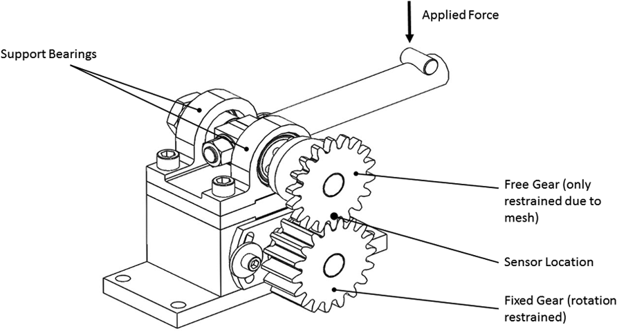
Gear tooth fatigue test rig.

For this work, the load applied was varied between 100 and 1400 N at a rate of 1 Hz. This load range was determined previously using a finite element model of the gear.¹² The loading frequency was limited by the characteristics of the servo-hydraulic load machine used for this work. The gear tooth in mesh on the free gear had a small notch (a 90° vee-shaped notch of approximately 1 mm depth, produced by trepanning with a lathe tool) cut at the junction between its fillet root and the involute profile in order to act as a stress concentration, thus ensuring that a fatigue crack would initiate at this location.

A strain gauge was mounted across the gear tooth fillet root, to act as an indicator of crack growth. This was combined with visual observation during the later stages of the test.

AE signals were collected by a Pancom P15 sensor (50–500 kHz) coupled to the free gear adjacent to the tooth under test using cyanoacrylate adhesive, connected via cable to the AE data acquisition system. The data were recorded by a MISTRAS group PCI 2 data acquisition system. The sensitivity of the data acquisition equipment was ensured by investigating the response of the system to a Hsu–Nielsen source.^16,17 Two categories of data were recorded: conventional AE data such as energy and hits (discussed further in section ‘Conventional AE’) and complete wavestreams captured over one loading cycle. These wavestreams capture the sensor output without any interpretation by the data acquisition system and are independent of threshold. Each wavestream was collected every 10 cycles, using a micro-switch mounted such that the loading arm operated the switch once per loading cycle; a decade counter linking the micro-switch and the AE acquisition system was utilised. Wavestreams were sampled at 2 MHz, 16-bit resolution and a duration of 1 s, which covers one complete tooth loading cycle.

Results

Periodic visual observations of the tooth were carried out. These observations identified a crack at approximately 22,000 cycles (this was further confirmed by strain gauge measurements, discussed in section ‘Strain gauge signals’). The test continued until approximately 28,000 cycles, when the crack was well established. Since the purpose of the test was to capture data in order to develop methods for the early detection of tooth fillet root cracking, it was not deemed necessary to continue the test until the tooth had completely fractured from the main gear body.

The recorded AE data were analysed in a conventional manner which is discussed in section ‘Conventional AE’, followed by a detailed analysis of the wavestream data in section ‘Wavestreams analysis’ and advanced AE signal analysis in section ‘Advanced AE on wavestreams’.

Strain gauge signals

The strain gauge voltage was logged by the PCI 2 system whenever an AE hit was detected. The strain gauge showed no increase in strain until approximately 23,000 cycles, as can be seen in Figure 2.

Figure 2.

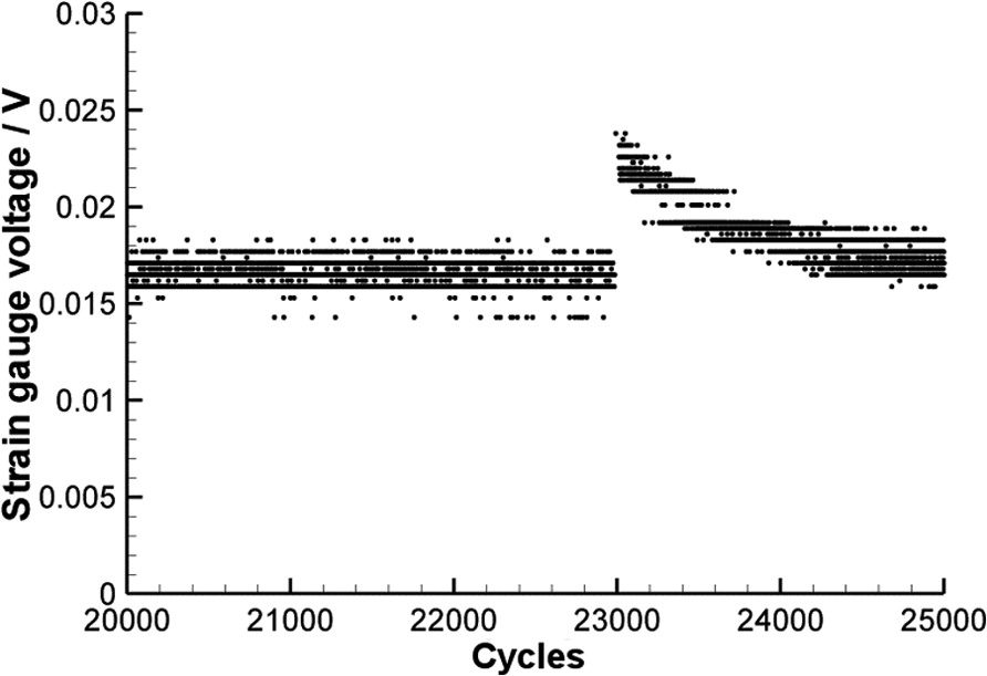
Strain gauge data for 20,000–25,000 cycles.

The strain gauge shows a significant increase in voltage output at approximately 23,000 cycles, suggesting that the crack observed visually at 22,000 cycles had reached the strain gauge location at that time. Although the strain appears to subsequently reduce, it is believed that this is due to the crack cycling damaging the strain gauge bonding, hence reducing the strain level back to previous lower levels. This was confirmed by inspection of the gauge post-test.

Conventional AE

Conventional AE analysis uses a series of metrics to describe the received AE signals above a user-defined threshold, in terms of parameters such as energy, amplitude, timing (i.e. rise to peak and duration) and counts (number of threshold crossings during the signal). In theory, during a fatigue test, when a crack is not growing, the amount of energy detected will remain constant on a cycle by cycle basis as this will be due to background noise from the test machine and other AE sources. Thus, one would expect the accumulated energy trend, plotted in Figure 3, to follow a linear rise due to background noise unless a crack or other new source of AE was present. However, when a fatigue crack develops, a new source of AE energy will be present, changing the rate of energy detected and providing an indication of the onset of cracking. A similar pattern should be expected for the number of detected signals which pass a pre-defined threshold of 45 dB (known as a hit).

Figure 3.

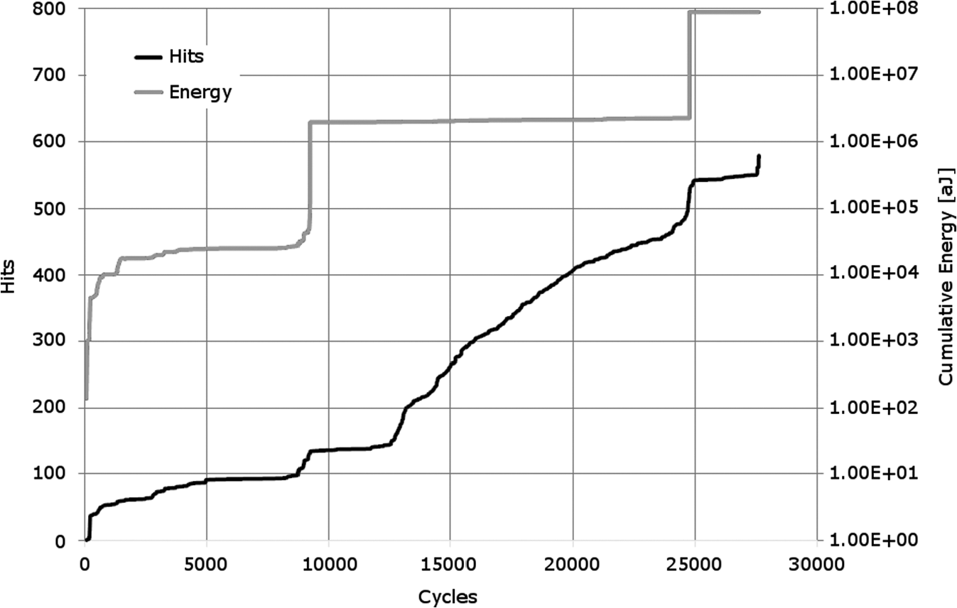
Conventional AE analysis based on energy and detected signals.

Figure 3 shows a large increase in energy at approximately 8500 and 25,000 cycles, which is in apparent contradiction with strain gauge data shown in Figure 2. This will be discussed further in section ‘Discussion’.

Wavestreams analysis

In order to further investigate the development of the tooth crack, the recorded wavestreams were analysed in detail. Four example wavestreams, at 5000 cycles, 16,400 cycles, 23,000 cycles and 26,300 cycles, are shown in Figure 4. Visual analysis of the signals does not clearly indicate significant differences in the signals over the duration of the test and is impractical from the point of view of a condition monitoring system. Therefore, some other means of quantifying the signal evolution in time must be used.

Figure 4.

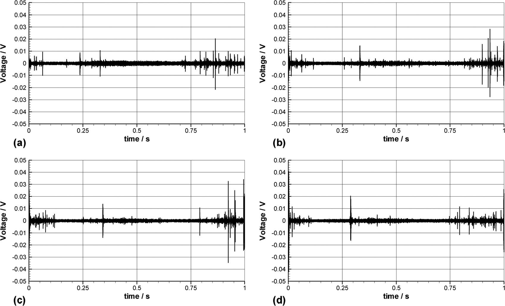
Example wavestreams recorded during test. (a) 5000 cycles, (b) 16,400 cycles, (c) 23,000 cycles and (d) 26,300 cycles.

The signals show a number of transient spikes, which are likely to be related to frictional sources due to the meshed teeth sliding relative to each other as the load is applied. Further sources of AE during the later stages of the test are likely to be due to crack nucleation and propagation. It is unlikely that sources due to crack face closure/rubbing are present since the crack location is always loaded in tension during this test.

Rolling cross-correlation

Cross-correlation is used to compare two signals – identical signals will return a normalised cross-correlation value of 1, while signals which are totally different would return a value of 0. Nominally, assuming that the first wavestream represents a baseline (undamaged) state, it can be expected that the cross-correlation will decrease as damage progresses; however, this approach did not provide sufficiently insightful results. A rolling cross-correlation was used instead, where every wavestream is compared to its immediate predecessor. The results of this analysis are shown in Figure 5.

Figure 5.

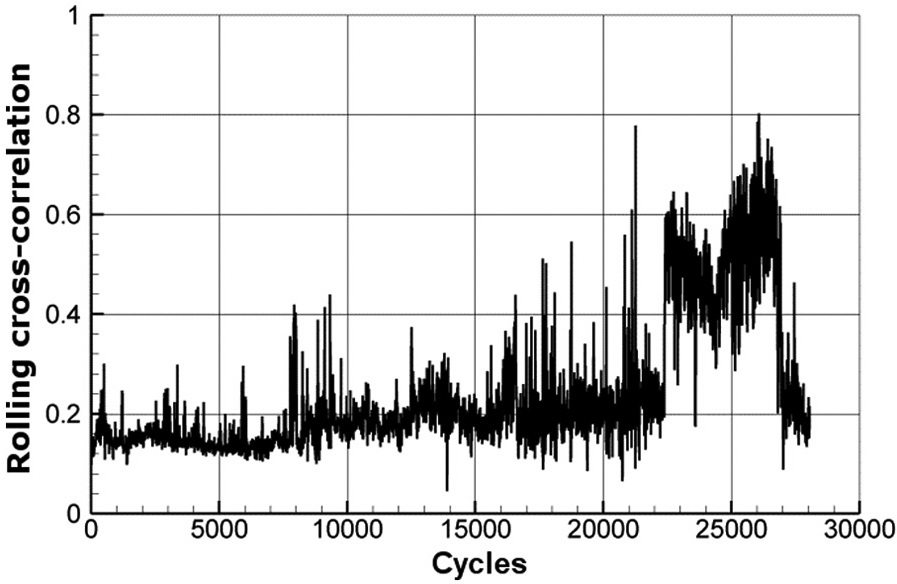
Rolling cross-correlation of wavestreams.

A rise in the rolling cross-correlation coefficient can be seen at around 23,000 cycles, and a low correlation coefficient before. This apparently counterintuitive result will be discussed in section ‘Discussion’.

Banded fast Fourier transform

A fast Fourier transform (FFT) analysis was performed on each of the approximately 2800 recorded wavestreams. The results of these FFTs were then banded – that is, all signals within a particular frequency band were considered separately. This approach is more suited to the analysis of components with complex geometries (such as gear teeth) where signal paths to the sensor may be subject to attenuations, than merely tracking the level of a particular frequency or set of frequencies. The tracking of banded frequencies allows discrimination between background noise (which would not evolve with time) and signals due to defects (i.e. crack growth in this case) which, it is reasonable to expect, would evolve with time. This approach has previously been found to be useful for the monitoring of rolling element bearings.¹⁸

Figure 6 shows FFT results divided into bands of 20 kHz width, and the maximum power within that band is tracked over the evolution of the test. Using total power in each frequency band yields similar, although less clear, indications and these results are therefore not presented.

Figure 6.

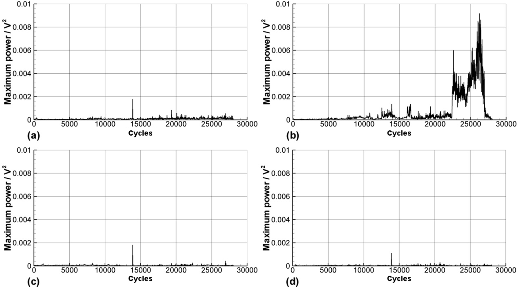
Maximum power obtained from banded FFT power spectra. (a) 80–100 kHz, (b) 100–120 kHz, (c) 120–140 KHz and 140–160 kHz.

Figure 7 further illustrates the approach. Here, the data are banded in 10 kHz steps between 60 and 200 kHz. The figure illustrates the total power within each band, calculated using the same method as the data shown in Figure 6. Activity levels within the 110- to 120-kHz band can be seen to increase from approximately 8000 cycles onwards, with a further significant increase in total power in this band from approximately 22,000 cycles.

Figure 7.

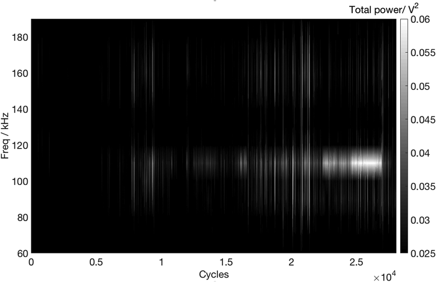
Total power from FFT spectra, banded between 60 and 200 kHz.

It is clear that the frequency content of the received signals varies throughout the test, but it must be appreciated that the measured signal is affected by the transfer function between the source and the acquisition system. For example, the relatively low power content throughout the test at around 130 kHz can be attributed to the sensor’s frequency response, which has a region of relatively reduced sensitivity centred around 130 kHz. For this reason, the frequency content of a measured signal must be interpreted in relative terms.

Advanced AE on wavestreams

Chebyshev moments as waveform descriptors

AE wavestreams are inherently difficult to handle. The high amount of data makes the manual inspection of time history plots an arduous task and prone to operator interpretation. Some traditional parameters such as energy, RMS and peak amplitude may result in false negatives, as they are not necessarily sensitive to short duration AE events occurring within a long wavestream.

One of the main challenges is also to be able to compare a wavestream collected at any given time with a ‘baseline’ wavestream collected when a structure or system is considered healthy. As ‘The assessment of damage requires a comparison between two system states’,¹⁹ it is clear how being able to measure some form of difference between a baseline signal and a measurement is necessary, and it can provide a form of measure of the deviation from the standard operating conditions.

Time–frequency information has been shown to carry significant information in the study of wavestreams. Certain frequency bands can be monitored for changes throughout a test. A challenge with this approach is to develop methods capable of discerning often subtle changes in signals.

Some more advanced processing techniques may be of use in this case. For example, wavelet decomposition has shown good results in describing and interpreting AE signals.^20,21 A reconstruction of the wavelet decomposition of a signal, in particular, can be used as a form of time-frequency transform, where each wavelet level is more sensitive to certain frequencies within a signal. Here, we propose a signal comparison technique, already preliminarily demonstrated on acousto-ultrasonic signals,²² that utilises the wavelet reconstruction of a signal to compose a time–frequency ‘image’ of said signal. Then, the moments of the Chebyshev polynomial decomposition of each wavelet reconstruction are computed. These moments can be used as descriptors and, if two sets of moments are compared, their correlation coefficient can be used as a measure of difference.^23,24

The Chebyshev moments calculation procedure is as follows:

Sample a discrete waveform d_i with $i = 1 \to N$ points;

Compute a discrete wavelet transform using M detail levels (Daubechies 10²⁵ in this case);

Reconstruct the wavelet details into a N × M matrix W;

Rectify the wavelet reconstruction row-wise: $D_{i} = | W_{i} |$ ;

Compute the Chebyshev moments of D up to the desired degree L.

Steps 2–4 produce a virtual image (matrix) of the one-dimensional waveform, where each row represents a wavelet detail level (which approximates a frequency band). The rectification is then used to avoid any dependency on initial phase or waveform slope.

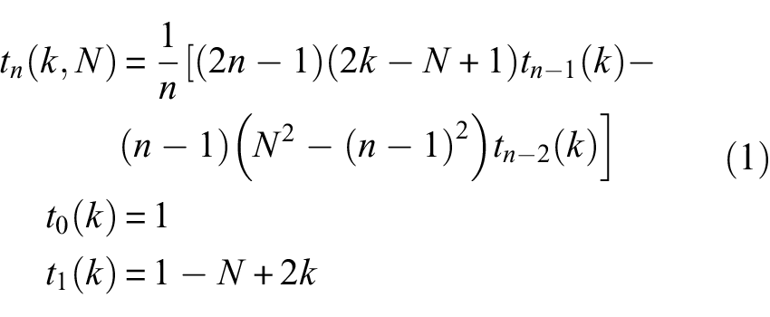
Discrete Chebyshev polynomials of degree n for a N points discrete signal t(k, N) can be expressed in the following recursive form, from the known values of t₀ and t₁, and k = 1 to N

\begin{array}{l} t_{n} (k, N) = \frac{1}{n} [(2 n - 1) (2 k - N + 1) t_{n - 1} (k) - \\ (n - 1) (N^{2} - {(n - 1)}^{2}) t_{n - 2} (k)] \\ t_{0} (k) = 1 \\ t_{1} (k) = 1 - N + 2 k \end{array}

(1)

The Chebyshev moment of order m + n for a N × M matrix D(i, j) is defined as

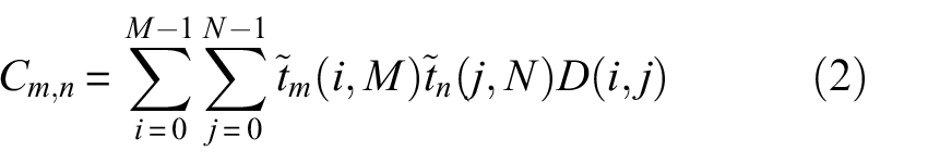
C_{m, n} = \sum_{i = 0}^{M - 1} \sum_{j = 0}^{N - 1} {\tilde{t}}_{m} (i, M) {\tilde{t}}_{n} (j, N) D (i, j)

(2)

where $\tilde{t}$ is the normalised Chebyshev polynomial defined as

{\tilde{t}}_{n} (k, N) = \frac{t_{k} (k, N)}{\sqrt{ρ (n, N)}}

(3)

and the normalisation factor ρ is defined as

ρ (n, N) = (2 n)! (\begin{matrix} N + n \\ 2 n + 1 \end{matrix})

(4)

After the computation of L-degree Chebyshev moments, a set (vector) of L² descriptors is obtained for every waveform. As the value of L increases, the set of moments will carry more detail about the representation of the signal. For this purpose, L = 5 has been chosen to represent signals, as the ratio between the higher degree, smaller moments and the lower degree, higher moments becomes small (approximately 10⁻³). This choice is empirical and is based on the observation that adding more moments increases computational time without adding useful information for the further steps. As previously explained, correlating these descriptors across two waveforms provides a measure of the similarity of two waveforms.

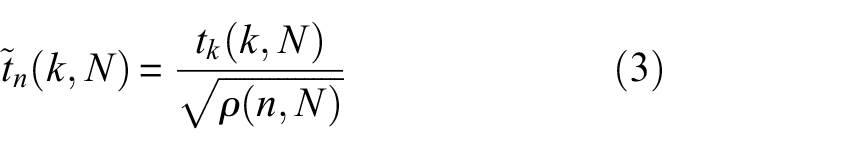
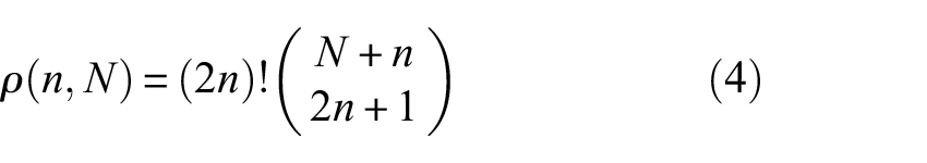
In order to demonstrate the technique, three waveforms obtained from a Hsu–Nielsen pencil-lead break source are considered (Figure 8(a)). Waveforms 1 and 2 are considered a good reference, while waveform 3 is the result of a ‘double break’ reference and should be discarded in a calibration dataset. Each waveform is, as per procedure, decomposed with a Daubechies 10 transform up to level 8 (Figure 8(b)).

Figure 8.

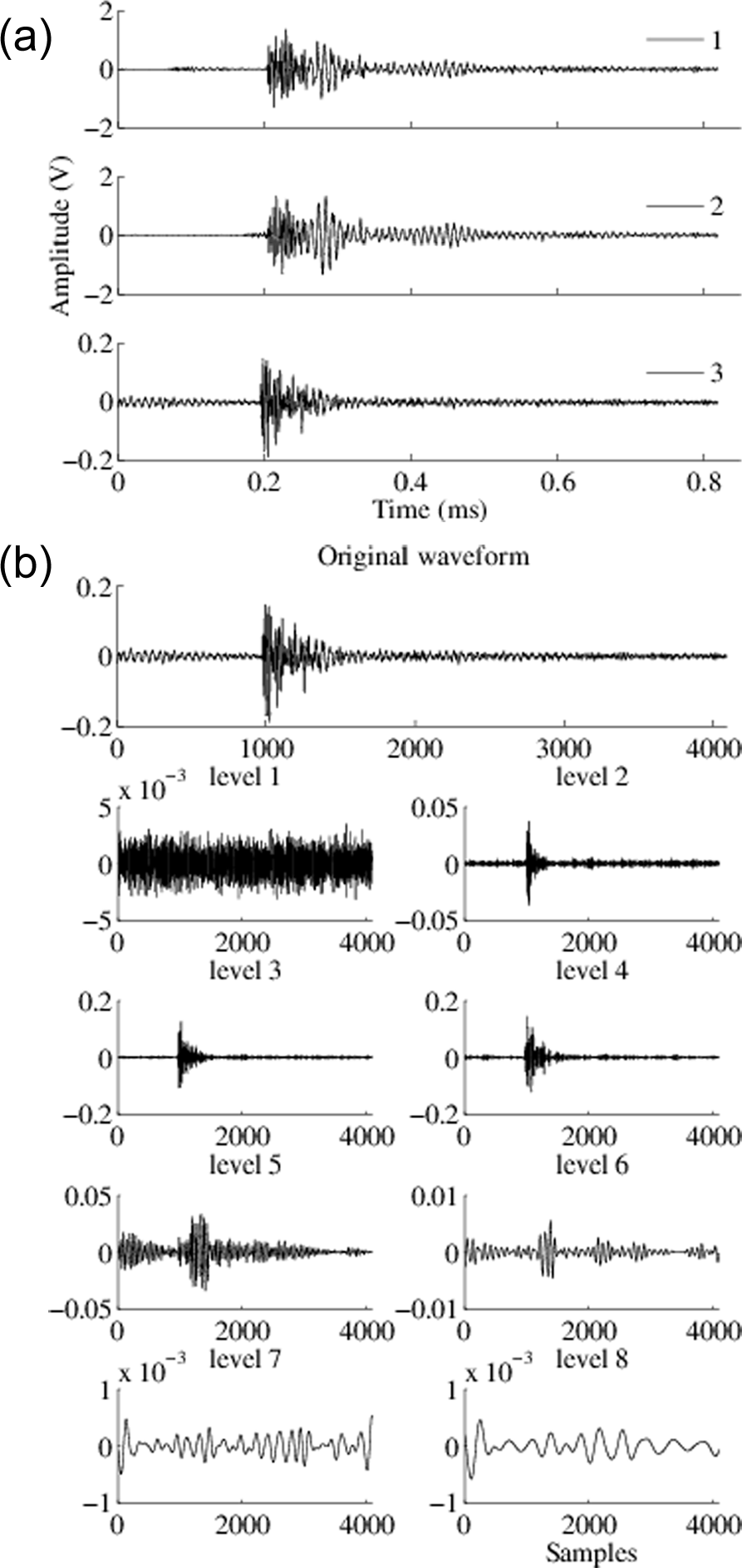
(a) Reference waveforms and (b) wavelet decomposition of waveform 1.

The Chebyshev moments of the wavelet reconstruction matrix are then computed and compared. Figure 9 shows a comparison of the Chebyshev moments of the three waveforms: waveforms 1 and 2 almost lie on the x = y line, meaning their moments are similar (Pearson’s correlation coefficient ρ = 0.99). Waveforms 1 and 3 have a significantly lower correlation coefficient, ρ = 0.85.

Figure 9.

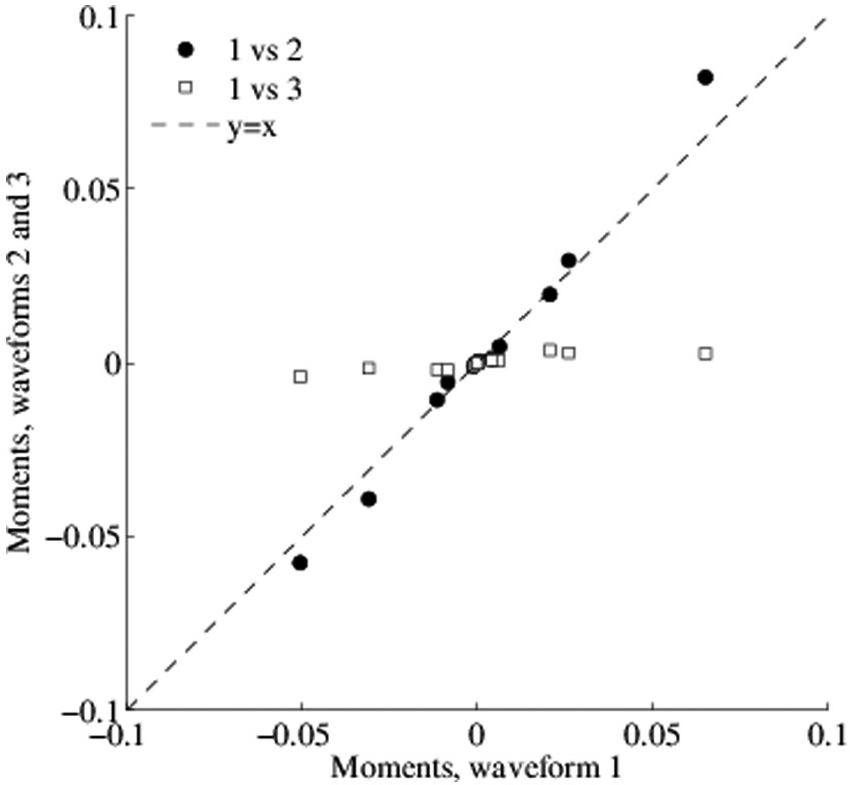
Comparison between Chebyshev moments of the three sample waveforms.

Chebyshev moments (N = 5) have been extracted for each wavestream. The choice of N depends on the level of detail that is deemed to be sufficient when using Chebyshev descriptors. Due to their nature, at increasing values of N, higher order Chebyshev moments tend to have smaller values; as a rule of thumb when the ratio between the maximum and the minimum Chebyshev moment is below 0.01, the cross-correlation plots show no visible change. Table 1 shows how for this experiment N = 5 satisfies the above relationship.

Table 1.

Normalised Chebyshev moments for wavestream number 1000.

C/max (C)	1.0000	0.6639	0.3133	0.1820	0.1458	0.1259	0.1169	0.0861	0.0700
	0.0679	0.0631	0.0507	0.0431	0.0384	0.0354	0.0284	0.0282	0.0273
	0.0257	0.0115	0.0096	0.0060	0.0038	0.0027	0.0012

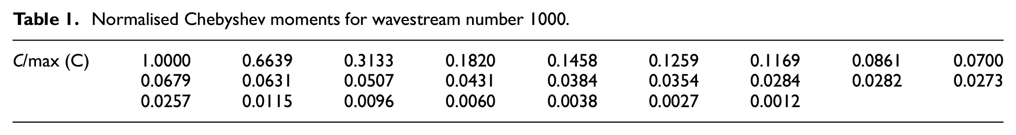
Figure 10 shows the correlation coefficient between wavestream number 100 (considered as a baseline once any initial settling of the test setup had taken place) and each other individual wavestream’s moments. As explained in the previous section, the Chebyshev moments correlation coefficient can be interpreted as a measure of the similarity between two waveforms. It is hence clear that from approximately 8000 cycles, the wavestreams start to diverge from the baseline.

Figure 10.

Correlation coefficient of Chebyshev moments of wavestream number 100 and all other wavestreams.

An efficient way to compute the correlation coefficient is via the correlation coefficient matrix. Here, each row and column represents a wavestream, and each (i, j) matrix position represents the correlation coefficient between wavestream i and wavestream j. The diagonal elements (i, i) are therefore equal to 1 (each wavestream correlates perfectly with itself).

Figure 11 shows the correlation coefficient matrix. Figure 10 can be viewed as a cross-section of Figure 11 taken at row 100 or at column 100.

Figure 11.

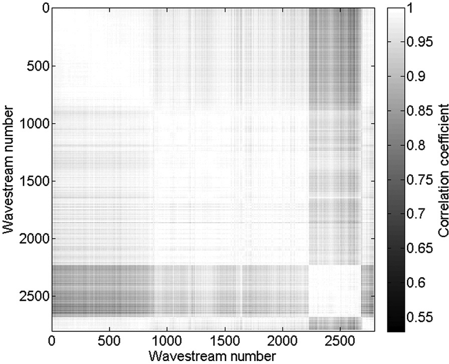
Correlation coefficient matrix for Chebyshev coefficients.

Signal entropy as indicator of damage

Shannon²⁶ entropy, in signal theory, can be seen as a measure of the content of information of a dataset. It is a scalar defined as

S = - \sum_{i = 1}^{n} p_{i} \times \log (p_{i})

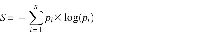
where p is the probability mass function of the N-point signal, and n is the number of possible values the signal can assume. In this particular case, n = 2¹⁶. Low levels of entropy means a higher level of predictability of the signal (i.e. the signal is mostly from a narrow and uniform distribution, such as noise) or, at the lower limiting case, it will be equal to 0 when the signal is completely certain (i.e. the signal is constant). Entropy will increase as soon as the signal becomes less predictable, or, in other words, carries more information.

In this work, a rolling entropy approach has been used. A sliding window of, in this case, 10,000 samples was used. The entropy value for each window was computed, and the maximum entropy within each collected wavestream was extracted: for an M point wavestream and an L sized window, and assuming p_i is computed within the moving window, the wavestream maximum entropy S_WS is computed as

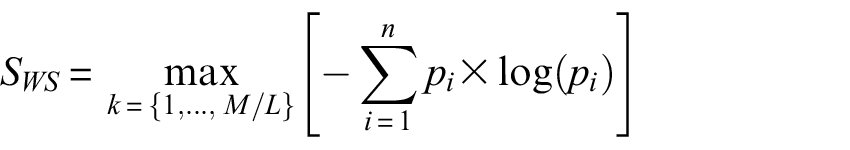
S_{W S} = \max_{k = {1, \dots, M / L}} [- \sum_{i = 1}^{n} p_{i} \times \log (p_{i})]

Figure 12 shows the entropy of an individual wavestream. The entropy is computed using a 10,000 samples sliding window. Using different sized windows ranging between 1000 and 10,000 samples (0.5–5 ms) did not highlight significant differences in the entropy shape and values. The window size should be sufficiently large that it captures the duration of one typical transient wave. Conversely, the window should be kept short enough to minimise the chance of multiple transients to be found within the same window, in order to better characterise wavestreams. For this test, a 5-ms window (10,000 samples) was found to be a good compromise between providing enough detail and minimising the computational effort. The maximum entropy value for the wavestream is highlighted and stored for each individual wavestream.

Figure 12.

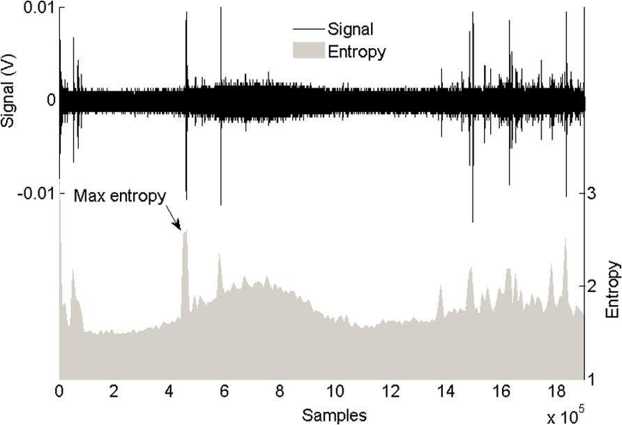
Entropy content of an individual wavestream (rolling window of 10,000 samples).

As each wavestream represents one loading cycle, statistical descriptors (mean, maximum and standard deviation) of entropy content were extracted. Maximum entropy, in particular, can be used to capture information about isolated high entropy transients. This approach differs from techniques such as envelope peak tracking, as the amplitude of the signal can be highly affected by source location. As Figure 12 shows, the isolated sharp signal occurring early in the time history (in this case likely to be attributed to crack propagation) has a higher entropy content than the packet of signals found at nearer the end of the time history. Other entropy statistical moments did not appear to add any significant diagnostic information.

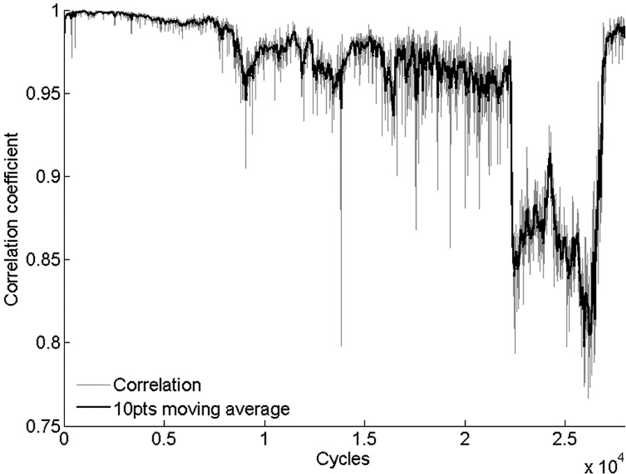
All collected AE wavestreams were processed. Figure 13 shows the maximum entropy trend during the test and the same values when averaged with a 10-pt moving average filter. Mean and standard deviation of entropy showed no appreciable sensitivity to detect or ability to highlight changes in the system.

Figure 13.

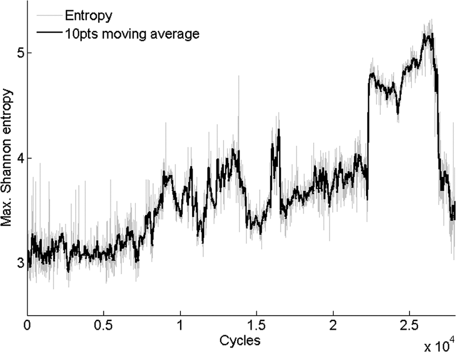
Maximum entropy per wavestream during the test.

Discussion

Rolling cross-correlation (Figure 5) shows a generally low level of cross-correlation values throughout the test; the value increases to around 0.8 at approximately 22,000 cycles, where the crack was believed to have significantly propagated according to strain gage signals and visual observations. These values can be explained when it is considered that earlier wavestreams essentially contain less deterministic signals such as those due to friction and loading machine noise, which are not repeatable across different wavestreams with respect to their temporal location. These display little consistence – one wavestream containing friction and other random sources is not necessarily similar to another wavestream, especially when the cross-correlation is computed on the full wavestream. Once a crack starts to grow, consistent signals are recorded within each wavestream, leading to a rise in the cross-correlation coefficient. This is believed to be related to the crack opening/propagating at similar load levels on each cycle, hence generating a more repeatable signal. Results shown in Figure 5 are however not clear and the technique is likely to be less applicable to situations where there are multiple sources of AE signals and the crack propagation and loading modes vary within a loading cycle.

Banded FFT and FFT imaging (Figures 6 and 7) show that the 100- to 120-kHz band is of significance in detecting cracking within the gear tooth. There is a very clear increase in the maximum power within the band at approximately 22,000 cycles. It is also arguable that there is more AE activity in this band than other bands between 8000 cycles and 22,000 cycles.

The application of the Chebyshev moments correlation produced interesting results. Figure 10 shows clear indications of wavestreams diverging from the baseline (no propagation) at about 8000 cycles and a high degree of change at 22,000 cycles. Figure 11 demonstrates that the wavestream features at 22,000 cycles are then similar with themselves until about 26,000 cycles; this indicates that a repeatable damage phenomenon is occurring.

Entropy calculation provided the same information but by retaining a single parameter in each waveform, that is the maximum Shannon entropy encountered in the individual wavestream. A steady increase in entropy starting at 8000 cycles is shown and is probably an indicator of increasing number or intensity of damage-like signals within a single wavestream. The same abrupt increase is then seen at 22,000 cycles, which matches the other techniques and visual observation. This matches traditional AE results which show a sharp rise in the energy parameter at the same number of cycles. Entropy however continues to rise until 15,000 cycles, hinting at an AE activity similar to the phenomenon that started at 8000 cycles. This also matches the Chebyshev correlation plot in Figure 11, showing a high degree of internal similarity in the 8000–15,000 cycles region.

Conclusion

While AE monitoring of rotating machinery is still challenging, this work shows that the technique is capable of early detection of crack propagation stages when supported by appropriate signal processing techniques: frequency power spectra analysis, wavestream features correlation and entropy proved to be good indicators for condition monitoring purposes.

Reducing memory footprint in a diagnostic system is a key in saving weight, reducing cost and limiting power consumption. The calculation of Chebyshev descriptors is computationally inexpensive and has a very small memory footprint: a waveform of 2 million datapoints can be discarded immediately after the calculation of a vector of 25 parameters, without the requirement to retain the entire waveform for subsequent comparisons. The technique allows a wavestream to be fingerprinted, and the descriptors have proven to be sufficient to describe the system deviation from a baseline state under the proposed experimental conditions.

The proposed Shannon entropy calculation showed good results in detecting the early and the late stages of damage while dramatically reducing the data footprint. However, the method produced results with a higher level of noise than the Chebyshev descriptors.

AE monitoring of rotating machinery is possible; this article lays the base for showing the detectability of tooth root cracking in a controlled experiment where the crack propagation was isolated from other sources. The synergistic use of the various techniques presented in this article has proven useful to explain the different phases of failure that the part under test has experienced.

Upcoming research will address the challenges related to AE monitoring of rotating gears with the techniques demonstrated and established in the present work.

Footnotes

Acknowledgements

The authors would like to acknowledge the support of MISTRAS Group Ltd and the technical staff of the Cardiff School of Engineering, in particular Paul Farrugia and Denley Slade, for the development of the decade counter micro switch triggering system.

Declaration of conflicting interests

The author(s) declared no potential conflicts of interest with respect to the research, authorship and/or publication of this article.

Funding

The author(s) disclosed receipt of the following financial support for the research, authorship, and/or publication of this article: The author(s) acknowledge the support of EPSRC Grant reference EP/L021757/1 which facilitated this work in part.

Data Access Statement

Information on how to access the data that supports the results presented in this article can be found in the Cardiff University data catalogue at

References

Wong

. Vibration-based helicopter gearbox health monitoring: an overview of the research program in DSTO. In: Proceedings of the DSTO international conference on health and usage monitoring (ed GF

Forsyth

), Melbourne, VIC, Australia, 19–20 February 2001, pp. 1–12. Melbourne, VIC, Australia: Defence Science and Technology Organisation.

Decker

. NASA-TM2002-211491: gear crack detection using tooth analysis. National Aeronautics and Space Administration, 2002.

Decker

. NASA-TM2002-211492: crack detection of aerospace quality gears. National Aeronautics and Space Administration, 2002.

Larder

. Helicopter HUM/FDR: benefits and developments. In: Proceedings of the American helicopter society 55th annual forum, Montreal, QC, Canada, 25–27 May 1999, pp. 1839–1846. AHS International.

Mc Coll

. Overview of transmissions HUM performance in UK North Sea helicopter operations. In: Proceedings of the IMechE seminar on rotor transmission system health monitoring: experience update, London, 19 November 1997.

Loutas

Sotiriades

Kalaitzoglou

et al . Condition monitoring of a single-stage gearbox with artificially induced gear cracks utilizing on-line vibration and acoustic emission measurements. Appl Acoust 2009; 70: 1148–1159.

Toutountzakis

Tan

Mba

. Application of acoustic emission to seeded gear fault detection. NDT&E Int 2005; 38: 27–36.

Tan

Mba

. Identification of the acoustic emission source during a comparative study on diagnosis of a spur gearbox. Tribol Int 2005; 38: 469–480.

Tan

Mba

. Experimentally established correlation between acoustic emission activity, load, speed, and asperity contact of spur gears under partial elastohydrodynamic lubrication. Proc IMechE, Part I: J Systems and Control Engineering 2005; 219: 401–409.

10.

Loutas

Kalaitzoglou

Sotiriades

et al . A novel approach for continuous acoustic emission monitoring on rotating machinery without the use of slip ring. J Vib Acoust 2008; 130: 064502.

11.

Carboni

Bruni

Crivelli

et al . A study on the performance of acoustic emission and low frequency vibration methods to the real-time condition monitoring of railway axles. In: Proceedings of the 12th international conference of the slovenian society for non-destructive testing, Portorož, Slovenia, 4–6 September 2013, pp. 559–566. The Slovenian Society for Non Destructive Testing.

12.

Pullin

Clarke

Eaton

et al . Detection of cracking in gear teeth using acoustic emission. Appl Mech Mater 2010; 24–25: 45–50.

13.

Fernandes

PJL

. Tooth bending fatigue failures in gears. Eng Fail Anal 1996; 3: 219–225.

14.

Olsson

Olander

Öberg

. Fatigue of gears in the finite life regime – experiments and probabilistic modelling. Eng Fail Anal 2016; 62: 276–286.

15.

Savaria

Bridier

Bocher

. Predicting the effects of material properties gradient and residual stresses on the bending fatigue strength of induction hardened aeronautical gears. Int J Fatigue 2016; 85: 70–84.

16.

Hsu

. A mechanical AE simulator for system calibration and waveform analysis. In: Proceedings of the 16th meet US acoustic emission work group, Williamsburg, VA, 18–20 October 1976, http://scholar.google.com/scholar?hl=en&;btnG=Search&q=intitle:A+mechanical+AE+simulator+for+system+calibration+and+waveform+analysis#0 (1976, accessed 19 December 2014).

17.

ASTM E976:2010. A standard guide for determining the reproducibility of acoustic emission sensor response.

18.

Cockerill

Clarke

Pullin

et al . Determination of rolling element bearing condition via acoustic emission. Proc IMechE, Part J: J Engineering Tribology. Epub ahead of print 16 March 2016. DOI: 10.1177/1350650116638612.

19.

Worden

Farrar

Manson

et al . The fundamental axioms of structural health monitoring. Proc R Soc Lon Ser: A 2007; 463: 1639–1664.

20.

Hamstad

O’Gallagher

Gary

. A wavelet transform applied to acoustic emission. J Acoust Emiss 2002; 20: 39–61.

21.

Downs

Hamstad

O’Gallagher

. Wavelet transform signal processing to distinguish different acoustic emission sources. J Acoust Emiss 2003; 21: 52–69.

22.

Crivelli

Eaton

Pearson

et al . Chebyshev descriptors for SHM with acoustic emission and acousto ultrasonics. Int J Struct Integr 2014; 5: 202–213.

23.

Sebastian

Patterson

Ostberg

. Comparison of numerical and experimental strain measurements of a composite panel using image decomposition. Appl Mech Mater 2011; 70: 63–68.

24.

Yap

Raveendran

. Image focus measure based on Chebyshev moments. IEE Proc: Vis Image Signal Process 2004; 151: 128–136.

25.

Daubechies

. Ten lectures on wavelets. J Soc Ind Appl Math. Epub ahead of print January 1992. DOI: 10.1137/1.9781611970104.

26.

Shannon

. A mathematical theory of communication. Bell Syst Tech J 1948; 27: 379–423.

Gear tooth root fatigue test monitoring with continuous acoustic emission: Advanced signal processing techniques for detection of incipient failure