Sage Journals: Discover world-class research

Abstract

In order to overcome the difficulties in applying traditional time-of-arrival techniques for locating acoustic emission events in complex structures and materials, a technique termed ‘Delta-t mapping’ was developed. This article presents a significant improvement on this, in which the difficulties in identifying the precise arrival time of an acoustic emission signal are addressed by incorporating the Akaike information criteria. The performance of the time of arrival, the Delta-t mapping and the Akaike information criteria Delta-t mapping techniques is assessed by locating artificial acoustic emission sources, fatigue damage and impact events in aluminium and composite materials, respectively. For all investigations conducted, the improved Akaike information criteria Delta-t technique shows a reduction in average Euclidean source location error irrespective of material or source type. For locating Hsu–Nielsen sources on a complex aluminium specimen, the average source location error (Euclidean) is 32.6 (time of arrival), 5.8 (Delta-t) and 3 mm (Akaike information criteria Delta-t). For locating fatigue damage on the same specimen, the average error is 20.2 (time of arrival), 4.2 (Delta-t) and 3.4 mm (Akaike information criteria Delta-t). For locating Hsu–Nielsen sources on a composite panel, the average error is 19.3 (time of arrival), 18.9 (Delta-t) and 4.2 mm (Akaike information criteria Delta-t). Finally, the Akaike information criteria Delta-t mapping technique had the lowest average error (3.3 mm) when locating impact events when compared with the Delta-t (18.9 mm) and time of arrival (124.7 mm) techniques. Overall, the Akaike information criteria Delta-t mapping technique is the only technique which demonstrates consistently the lowest average source location error (greatest average error of 4.2 mm) when compared with the Delta-t (greatest average error of 18.9 mm) and time of arrival (greatest average error of 124.7 mm) techniques. These results demonstrate that the Akaike information criteria Delta-t mapping technique is a viable option for acoustic emission source location, increasing the accuracy and likelihood of damage detection, irrespective of material, geometry and source type.

Keywords

Acoustic emission source location structural health monitoring damage detection signal processing

Introduction

Structural health monitoring (SHM) systems allow in-service structures to be continuously monitored using the permanently mounted sensors and are akin to the human nervous system.¹ These systems allow for the early detection of damage and in the future, if applied appropriately, would enable damage characterisation and the calculation of the remaining life. With the increasing use of composite materials and ageing aircraft, the aerospace industry is one particular sector that would benefit from wide-scale application of SHM systems. A substantial proportion of aircraft non-operational ground time is due to scheduled and periodic inspections.² SHM systems allow maintenance to be conducted when required rather than based on operational hours. This increases asset use and reduces operating costs, resulting in the most efficient use of the aircraft while still maintaining reliability and safety.

Composites materials are susceptible to large internal defects which may not be visually detectable, significantly affecting the designed strength and component life.³ This leads to conservative designs resulting in heavier components and reducing the strength-to-weight ratio advantage of composite materials. The introduction of SHM systems at the design stage would remove the need for conservative design, leading to more optimised structures, reducing aircraft weight and improving performance. SHM systems can also be retrofitted to ageing aircraft and it is thought that the long-term benefit to maintenance could easily offset the initial outlay.³ These systems can be beneficially used to monitor inaccessible hotspot areas which are labour-intensive to inspect using conventional techniques due to the need for disassembly of components.

One particular non-destructive technique (NDT) that is particularly suited to SHM is acoustic emission (AE). AE is described as the rapid release of energy that propagates in a material in the form of an elastic stress wave due to permanent internal changes. A variety of mechanisms can give rise to AE, including crack initiation and propagation, plastic deformation, fretting, matrix cracking and fibre breakage. These stress waves cause minute displacements at the surface of the material that can be detected using piezoelectric sensors and are recorded on an acquisition system based on a user-defined threshold. AE is seen as a passive approach, essentially ‘listening’ to active sources within the structure.

AE source location

One advantage of AE for SHM is its ability to locate the source; the most common commercial algorithm for this is the time of arrival (TOA) method.⁴ However, due to the assumptions in the algorithm, significant errors can be introduced. One of these assumptions is that the structure is homogenous, and that the wave velocity is the same in all directions. This is certainly not the case in composite materials and complex structures where velocity varies with propagation angle, due to the fibre layup in composite materials or geometric features which give rise to an interrupted propagation path. The user-defined threshold technique to determine arrival times, common to commercial AE acquisition systems, can introduce significant errors in location accuracy due to attenuation, source amplitude and dispersion which make it difficult to determine the wave arrival time with precision.

There has been a vast amount of research focussed on addressing these assumptions and therefore improving source location. The proposed techniques can be categorised into the following groups: wave speed is known or unknown, specific closely spaced sensor arrays, statistical, beam-forming and mapping techniques.

Dispersion curves or experimentally derived wave velocities for different propagation angles are often utilised for location techniques that require prior knowledge of material wave speeds. Mostafapour et al.⁵ used wavelet decomposition, cross-time–frequency spectrums and the most energetic frequency velocity from dispersion curves to locate sources in a steel plate. Often the wave velocities in two principal directions are used to locate sources in the composite materials, such as the elliptical wave front triangulation method⁶ which was combined with Rayleigh maximum likelihood estimate⁷ to locate impacts in composite aircraft panels.⁸ Koabaz et al.⁹ used an experimentally derived wave velocity and developed the work of others¹⁰ to realise an improved objective function in an optimisation scheme to locate impacts on a composite panel. For structures with increasing complexity, Geiger’s method and a variable velocity model were used to locate micro-cracks in cemented total hip arthroplasty.¹¹

Often the use of dispersion curves or experimentally derived wave velocities is not practical in reality. Techniques have been developed that require no further knowledge of the material properties. Ciampa and Meo¹² used a specific triangular layout of six sensors arranged in three closely spaced pairs, reducing the number of non-linear equations, which were solved using Newton’s method. This technique was further applied to composite sandwich panels with an arbitrary layup.¹³

All the techniques discussed thus far have focussed on using sparsely distributed sensors and locating within the sensor array. Researchers have developed techniques that utilise specific closely spaced sensor arrays to enable global location outside the sensor array. Aljets et al.¹⁴ used three closely spaced sensors in a triangular array to locate sources globally in a composite plate. The propagating angle from the array was determined using the A₀ wave arrival time using a wavelet transform (WT) at a specific frequency. Knowing the maximum and minimum S₀ wave velocities for different propagating angles enabled the formulation of a numerical model. This, combined with the temporal separation of the two wave modes, determined the distance along the propagation angle using single sensor location techniques.¹⁵ Matt and Lanza Di Scalea¹⁶ used a rosette arrangement of three macro fibre composites sensors, exploiting the directional response of these sensors to determine the propagating angle of the flexural mode. Utilising at least two rosettes allowed source location in two dimensions. Kundu et al.¹⁷ used two clusters of a specific closely spaced triangular array of three sensors to determine the source location based on the intersection of the two calculated propagating angles. This technique required no prior knowledge of the wave speed. The introduction of an optimisation scheme using the initial estimate from the intersection further improved the technique.¹⁸

Delay and sum beam-forming is another technique that incorporates a closely spaced sensor array to determine global source locations which has been used on large-scale bridge structures¹⁹ and in metallic plates.²⁰ Xiao et al.²¹ used two linear sensor arrays to perform delay and sum beam-forming to give accurate source locations irrespective of wave velocity.

The majority of recent research has focussed on probabilistic source location estimates rather than deterministic solutions. This has allowed calculation of the source location confidence, and many researchers have incorporated Bayesian statistics. A Bayesian approach was used to estimate source locations in a concrete beam.²² A simplified predictive model was created which described the source location estimations using four parameters represented by a probability density function (PDF). Bayesian statistics and Markov chain Monte Carlo (MCMC) methods have been used with a ray tracing model to locate AE sources in liquid-filled storage tanks²³ and with data fusion techniques to locate sources on a stiffened aluminium panel.²⁴ Kalman filters have also been utilised for probabilistic AE source location. Extended Kalman filters (EKFs) alongside parameter extraction, binary hypothesis testing and data weighting were used as a data fusion approach to locate in noisy environments.²⁵ Both EKF and unscented Kalman filters (UKFs) were used to locate impacts on a composite plate for conditions where the wave velocity was known and unknown.²⁶ The UKF is seen as a performance improvement over the EKF.²⁷ The EKF can suffer from poor performance and diverge for highly non-linear problems due to the distribution being represented by a first-order linearisation of the system. The UKF addresses these problems by achieving the approximation through evaluating the non-linear function with carefully chosen sample points.²⁸ Niri et al.²⁹ used unscented transformation for source location and compared the results with MCMC methods using Kullback–Leibler divergence. The technique gave accurate results and required a lower number of samples. Although there are advantages of being able to determine the confidence bounds of the estimated source locations, these statistical approaches often take a large amount of processing time and at the moment would not be suited to real-time monitoring of actual damage mechanisms.

The final approach is the use of mapping techniques. Most solutions presented so far assume an uninterrupted source to sensor propagation path which may not be applicable in complex structures. The best matched point search method was developed by Scholey et al.;³⁰ an array of points was used to represent the geometry. Matching the theoretical and experimental difference in arrival times, by minimising the error, it was possible to estimate source location. Hensman et al.³¹ used a laser to generate artificial AE sources on a structure and the Akaike information criteria (AIC) picker to determine the arrival times; Gaussian processes were used to directly relate the difference in arrival times to Cartesian coordinates.

Onset picking

In order to reduce source location errors, accurate arrival time estimation is crucial. Traditionally, the first crossing threshold technique is used and consideration of the chosen threshold is of paramount importance. Reducing the threshold level can improve location accuracy; however, early triggering could occur. Filtering, WTs and statistical approaches have been used to improve source location accuracy. Cross-correlation has been used to calculate difference in arrival times by modulating the sensor output to emphasise the phase difference of a single frequency.³² Knowing that the peak of the wavelet coefficient at a particular frequency could be used to determine the group velocity paved the way for WT arrival time estimation.³³ Jeong and Jang³⁴ used this principle to locate Hsu–Nielsen (H–N) sources³⁵ on a large aluminium panel. However, the accuracy of WT arrival time picks becomes far less reliable in the presence of reflections from structural features and boundaries and its performance is poor at low signal-to-noise ratios.³⁶ Ding et al.³⁷ used wavelet decomposition to identify energetic frequencies within a signal at which they band-pass filtered the signal prior to arrival time detection by a threshold. The filter bands used were quite wide (150 kHz), and arrival times could still be picked at a range of different frequencies (and hence velocities); therefore, threshold crossing errors due to attenuation can still occur. Shehadeh et al.³⁸ presented a sliding window energy technique that uses a change in the ratio of signal energy above and below a user-defined frequency level. The sliding window energy technique was compared with wavelet, cross-correlation and threshold arrival time determination techniques to measure the wave speed in a long steel pipe. The sliding window energy technique was shown to compare most favourably to manual arrival time picks. However, the authors showed that the technique is sensitive to the splitting frequency selected and this is likely to vary for differing materials, sensors and sources. A method of automatically detecting the observed changes is also required.

Other researchers have focussed on the use of statistical methods to determine the first signal motion above background noise. Lokajicek and Kilma³⁹ utilised higher order statistics within a sliding window. When the window contained noise prior to signal onset, the distribution was normal. When signal samples were present in the sliding window, the distribution is distorted and the statistical moments are seen to change. The change in the derivative of the sixth-order statistical moment was detected using the ratio of the short-time average to long-time average (STA/LTA) approach⁴⁰ and an arrival time estimation accuracy of ±2 sample points was demonstrated for 95% of events when compared with manual picks. Kurz et al. utilised a modified form of AIC^41,42 proposed by Maeda for direct application to raw transient signals. The technique compares signal entropy before and after each point t in a signal and returns a minimum at the point of signal onset. This occurs when high-entropy uncorrelated noise prior to signal onset is compared with low-entropy waveform showing marked correlation after signal onset. A simple minimum finding function can then be used to determine the signal arrival time. Further details on the implementation of the AIC technique are given later in this article. The AIC technique was compared to the Hinkley⁴³ criteria, proposed by Grosse,⁴⁴ which computes the partial energy of the signal for each point i, and by applying a negative trend, a minimum is observed at the point of signal arrival. Kurz et al.⁴⁵ concluded that the AIC function was superior to the Hinkley criteria across a range of signal-to-noise ratios and showed that 90% of events were located within 5 mm of those computed from manual onset picking, compared with only 40% for the Hinkley criteria. Carpinteri et al.⁴⁶ showed similar performance of the AIC onset picker in concrete beam tests. Sedlak and colleagues^47,48 proposed a two-step AIC approach that resulted in computed locations that were on average within 1 mm of those computed from manual picks. It is questionable if the increased processing required is necessary, given the accuracy reported by others for the standard implementation of the AIC function.

Delta-t mapping

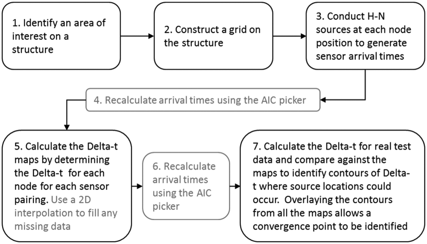
The traditional Delta-t mapping technique was developed by Baxter et al.⁴⁹ and was developed for source location in complex structures. It uses H–N sources to generate artificial AE signals in the structure in order to generate arrival times at the sensors. This creates maps of the difference in arrival time (Delta-t) between sensor pairs. Test data are compared to the training maps in order to estimate the source location. It was not envisaged that the technique would be used to monitor large structures but more focus on ‘hotspot’ areas with complex geometry or known stress concentrations. A summary of the main steps in the technique is given in Figure 1.

Figure 1.

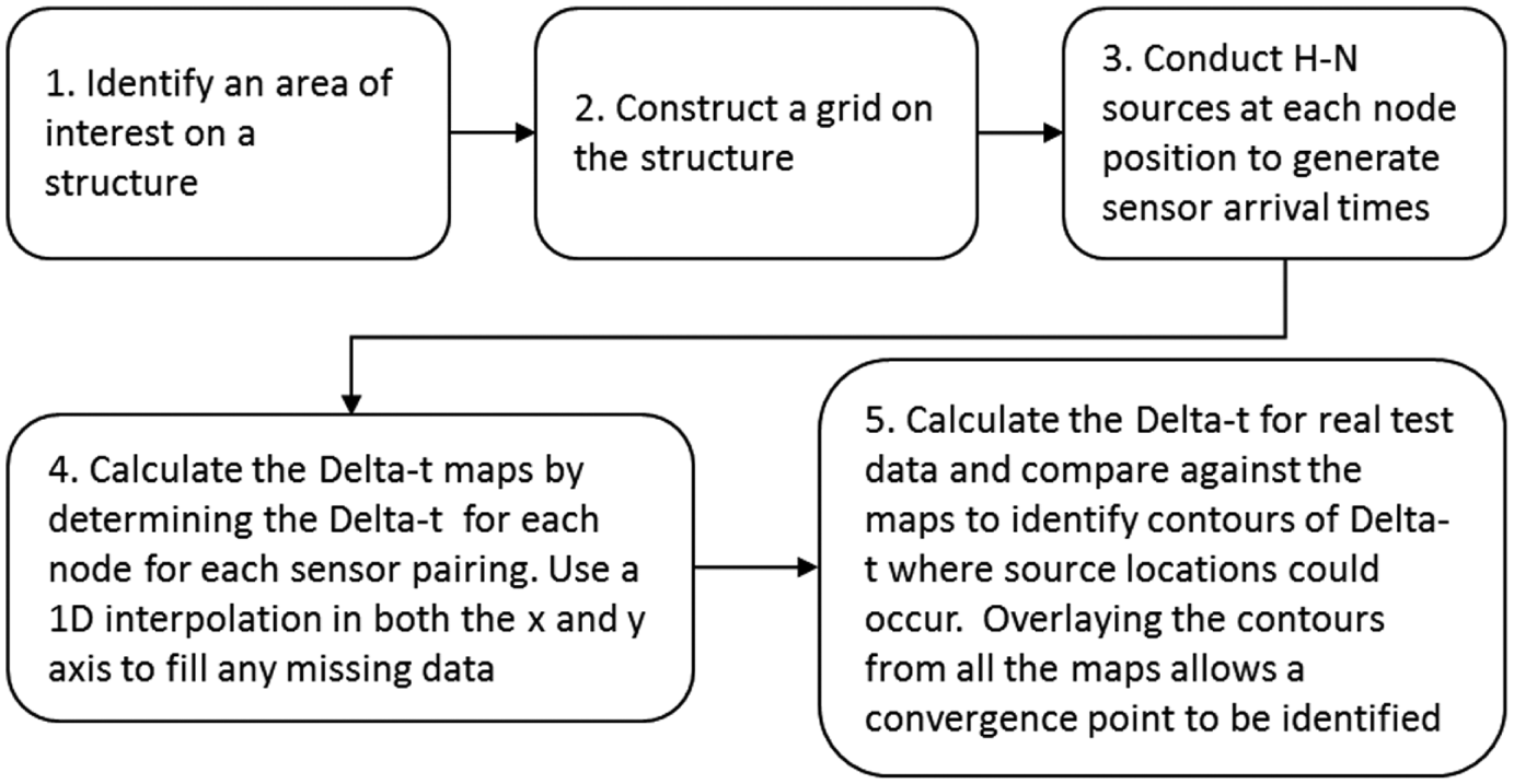
Delta-t mapping technique.

Baxter et al. showed that for locating H–N sources on an aircraft component, a reduction in error from 4.81% to 1.77% was observed when compared with the TOA technique. Further robustness testing and location of fatigue damage in composite structures have been demonstrated.⁵⁰ The major disadvantage of this technique is that the first threshold crossing technique defines the arrival times calculated at the sensors.

Improved AIC Delta-t mapping

It is proposed that significant improvement can be made to the Delta-t mapping technique by introducing a more robust approach to arrival time estimation. The AIC-based arrival time estimation discussed above is selected for use in this work for a number of reasons. Researchers have shown AIC to compare very favourably to manually picked arrival times and to consistently outperform other arrival time estimators (as discussed above). The AIC function returns a single minimum at signal onset that can be easily identified, with no ambiguity, by a simple minimum finding function. For many other arrival time estimators that detect a change in a particular metric at the signal onset time, there remains a requirement to automatically identify the point of change which commonly relies on thresholds that are inherently ambiguous. The AIC function operates with relatively low computational cost compared with more complex arrival time estimators, for example, those based on WTs. It has been shown to be robust across a range of signal-to-noise ratios and signal types. The main challenge in implementing the AIC approach is the selection of an appropriate window length over which to apply the function; too long and multiple minima may occur, and too short and sensitivity may be reduced. A detailed discussion of the implementation of the AIC function follows.

This work uses an adaptation of the AIC implementation described by Kurz et al.⁴⁵ Whereas Kurz utilised Hilbert and WTs to approximate the signal onset time prior to applying the AIC function to a reduced window, here the first threshold crossing from the raw transient was used as an initial approximate, thus further reducing computational demand. Kurz et al. then took a window of 400 samples prior to the approximate onset and 150 samples after approximate onset within which to apply the AIC function (equation (1)). Here, the same function is applied to a window from the waveform start (500 µs prior to threshold crossing) to 150 sample points after the threshold crossing.

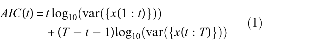
A I C (t) = t \log_{10} (var ({x (1 : t)})) + (T - t - 1) \log_{10} (var ({x (t : T)}))

(1)

Equation 1 shows the AIC function where var is the classic variance of a given vector. As can be seen, the AIC function splits the signal into two vectors, {x(1:t)} and {x(t:T}, and describes the similarity between them. When point t is aligned with the signal onset, the vector prior to t contains only high-entropy uncorrelated noise and the vector after t contains only low-entropy signal with marked correlation and the AIC function therefore returns a minimum. Figure 2 shows an implementation of this approach on a high-amplitude signal from an H–N source and a low-amplitude signal from a fatigue test with threshold crossing errors of a few samples, and approximately 100 samples are seen, respectively, further highlighting the potential errors that may occur when training Delta-t maps with a high-amplitude H–N source and then trying to locate a lower amplitude sources. Kurz et al. demonstrated their implementation to be robust across a range of signal-to-noise ratios and similar is found here with favourable comparison to manual picks observed for a variety of signals from differing sources, materials and sensor types. Table 1 compares 45 signals from a range of tests in an aluminium and composite specimen detailed in the experimental procedure. In practice, it is only the window size after the signal onset that is important for the AIC process, with 150 samples after onset coupled with varying sample numbers prior to the onset, that is, 500 µs at varying samples rates, still yielding accurate results (Table 1).

Figure 2.

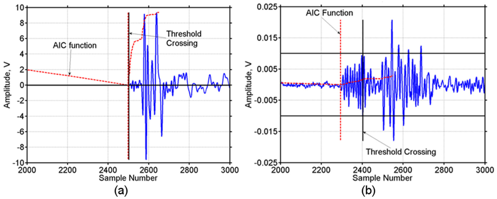
Arrival time comparison for (a) high- and (b) low-amplitude AE signals.

Table 1.

Arrival time estimation in terms of samples for TOA and AIC when compared with manual picking

Experimental test	TOA		AIC
	In terms of samples
	Average error	Standard deviation	Average error	Standard deviation
Aluminium specimen	65.5	129.9	2.6	3.0
Composite specimen	23.8	17.5	1.6	2.5

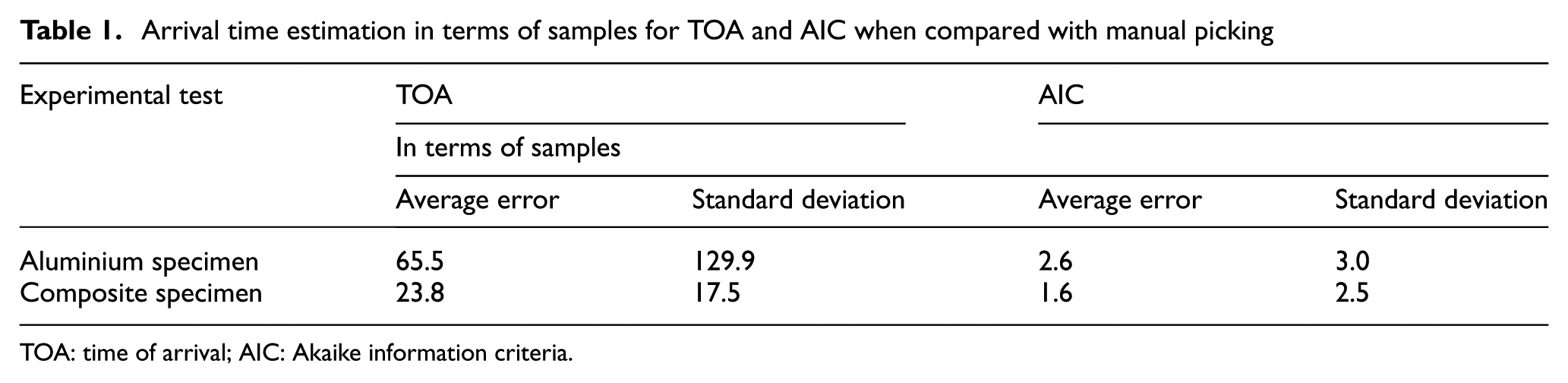
TOA: time of arrival; AIC: Akaike information criteria.

The steps in the improved AIC Delta-t mapping are outlined in Figure 3 with the improvements highlighted in grey. This article showcases the improvement of the AIC Delta-t technique over conventional TOA and the traditional Delta-t mapping technique for a variety of situations: locating H–N source in the composite and metallic structures, fatigue damage in an aluminium specimen and impacts in a composite specimen; it is the first time comparisons for all three technique have been made for locating a variety of source mechanisms in a variety of materials.

Figure 3.

Improved AIC Delta-t mapping.

Experimental procedure

Three experimental investigations were undertaken to demonstrate the performance enhancement of the AIC Delta-t mapping over the Delta-t mapping and TOA techniques. Typical aerospace damage mechanisms were investigated: fatigue cracking in aluminium and impact events in carbon fibre composite. An additional large-scale test was undertaken using H–N sources on a complex geometry aluminium aerospace component. These tests were devised to show the robustness of the AIC Delta-t for locating damage irrespective of material type, damage mechanism and component scale.

Aluminium fatigue specimen

A complex geometry specimen was manufactured from aerospace grade aluminium (2024-T3; Figure 4). The overall specimen dimensions were 370 × 200 mm with a thickness of 3.18 mm. A series of different diameter holes were machined into the specimen to ensure a complex and interrupted wave propagation path. For both the Delta-t mapping techniques, an area of interest was defined by placing a 200 × 160 mm grid on the structure with a nominal node spacing of 10 mm. In order to monitor any subsequent AE activity, four Mistras Group Limited (MGL) Nano 30 sensors (operating frequency of 125–750 kHz) were coupled to the specimen using silicon RTV (Loctite 595) and left to cure for 24 hours. MGL in-line preamplifiers with a gain of 40 dB were used alongside an MGL PCI-2 acquisition system. AE waveforms were recorded using a 40-dB threshold, 100–1200 kHz analogue filters and a 2-MHz sample rate. Prior to the testing, training data were collected for the Delta-t techniques. The training process for the Delta-t maps was completed once on the pristine sample and the subsequent location calculation of all damage events was undertaken using this single set of training data, without further updating. A series of five H–N sources were made at each grid position and this generated artificial AE sources enabling sensor arrival times to be determined. Load distribution into the specimen was achieved using 5-mm steel clamping plates, and a 20-mm pin attached the specimen to the hydraulic load machine. The specimen was loaded under tension–tension fatigue with a minimum load of 0.25 kN and a maximum load of 24 kN using a 2-Hz sinusoidal loading profile. AE data were continuously recorded throughout the fatigue testing.

Figure 4.

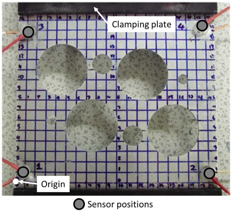
2024-T3 complex geometry specimen.

Composite impact specimen

Figure 5 shows the composite specimen used for the impact investigation, which was manufactured from Cytec MTM28-1/HS-135-34%RW with a ((0,90)₄)_s layup. The overall specimen dimensions were 370 × 185 mm and 2.15 mm thick. Figure 5 shows the area of interest (180 × 160 mm, 20 mm grid resolution), sensor positions (red circles) and impact site (red cross). Four Pancom Pico-Z sensors, with an operating frequency of 125–750 kHz, were mounted to the specimen using cyanoacrylate. In accordance with the aluminium fatigue investigation, the same in-line amplifiers and AE acquisition system were used; however, a 50-dB threshold, 20–1200 kHz analogue filters and a 5-MHz sample rate were used to record AE data. Prior to the impacts, five H–N sources were used at each node position within the grid to create the necessary data for the Delta-t mapping techniques. As with the aluminium fatigue specimen, the training data for the Delta-t maps were collected with the specimen in pristine condition and the single data set was used for all subsequent location calculations. The effectiveness of the training data for both techniques was evaluated by H–N sources at random grid positions. An ultrasonic C-scan was used to determine there were no manufacturing defects. The specimen was subjected to four impacts (3, 4, 5 and 5 J energy) at the same position of (40,65) mm from the bottom left-hand corner of the grid using an Instron Dynatup 9250HV impact test machine. During the impact testing, the sample was supported between two square clamping frames placed on either side of the specimen and centred about the impact location. The frames provide a 60 × 60 mm unsupported area and have an overall outer dimension of 100 × 100 mm. The rest of the sample remained unclamped throughout the impact testing. AE data were recorded during the impact events when the specimen was clamped in the arrangement described.

Figure 5.

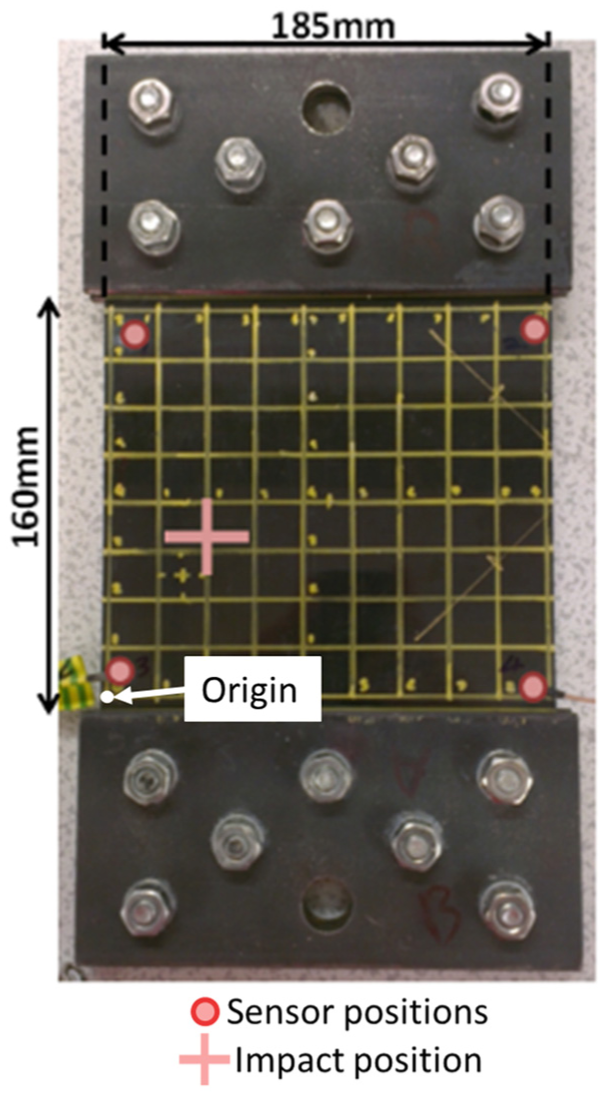
Composite impact specimen.

Aluminium aircraft panel

Figure 6(a) and (b) shows the complex geometry aluminium wing rib under investigation, with a 400 mm × 400 mm Delta-t grid applied at a grid resolution of 10 mm. The overall specimen dimension was 1.5 × 0.48 m. Figure 6(b) shows the reverse of the panel and shows the structural features present and their position with respect to the grid (dashed square). Four Mistras Nano30 sensors were mounted at the corners of the grid with coordinates of (−15,−8) mm, (413,−4) mm, (−7,405) mm and (415,402) mm with respect to the (0,0) grid position. The mechanical and acoustic coupling of the sensors was achieved using silicon RTV (Loctite 595) which was allowed to cure for 24 hours prior to testing. The sensors was connected to an AE acquisition system via amplifiers with a 40-dB gain and a 20–1200 kHz analogue filter. AE data was collected using a 40-dB threshold level and waveforms were recorded at a sample rate of 2 MHz. Training data were collected from five H–N sources performed at each node within the grid. To assess the effect of training data resolution, the data was then separated into training sets with grid resolutions of 10, 20, 50 and 100 mm, and Delta-t maps were prepared for each training data set. To assess the location performance, eight positions were selected within the grid that did not correspond to grid nodes (i.e. training data points) and five H–N sources were collected from each. Locations were computed using TOA, traditional Delta-t and AIC Delta-t for comparison.

Figure 6.

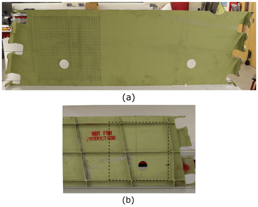
Aluminium aircraft panel showing the a) Delta-t grid and b) the structural features on the reverse of the panel.

Experimental results and discussion

H–N source investigations

In advance of using the Delta-t mapping techniques for damage location, the accuracy of the training data was assessed using H–N sources at random node positions. This allowed assessment of the training data quality and provided the opportunity to compare location techniques.

Complex fatigue specimen

Figure 7(a) shows the estimated source locations for three H–N sources at six random positions for the TOA, Delta-t and AIC Delta-t mapping techniques. Figure 7(b) shows the results of the average Euclidean distance error for each location position. The error bars in the figure represent the maximum and minimum errors for each position. This is the case for all the remaining figures. Both the Delta-t mapping techniques are able to resolve all six locations within the specimen geometry. The TOA technique is only able to locate four of the six locations within the specimen with locations for positions 1 and 6 located 52 and 90 mm outside of the structure boundary, respectively. This demonstrates the robustness of Delta-t mapping over the TOA technique and allows the user to be confident that all possible sources will be sensibly located. The AIC Delta-t mapping technique has located all but position 5 with an accuracy of less than 3 mm and in four of the six cases has outperformed the standard Delta-t approach, the exceptions being positions 1 and 3. In the case of positions 1 and 3, the AIC Delta-t mapping technique has an accuracy of less than 2.5 mm, with the standard Delta-t technique errors of 1.0 and 0.8 mm, respectively. However, if these differences are considered relatively to the uncertainty in the measurement chain, then they appear to be well within the expected noise. For example, placement of the H–N source is expected to be within 1–2 mm of the desired location (due to human error) and the Nano30 sensors used in the example have a radius of 4 mm. Additionally, assuming a wave speed of 5400 m/s (fastest propagating mode in this material) and a sample rate of 2 MHz, one sample error in arrival time is equivalent to 2.7 mm. So even if the first sample of the arriving wave is accurately picked, an error of up to 2.7 mm could still be expected. Coupling these together means that any fluctuations of less than ∼8 mm can be considered to be within the limits of uncertainty for this measurement. The largest error observed for the AIC Delta-t is seen at position 5 which is still within the suggested 8 mm uncertainty. The overall average Euclidean location errors for the three techniques are 32.6, 5.8 and 3.0 mm for the AIC Delta-t, Delta-t and threshold approaches, respectively, demonstrating the improved overall performance of the AIC Delta-t technique.

Figure 7.

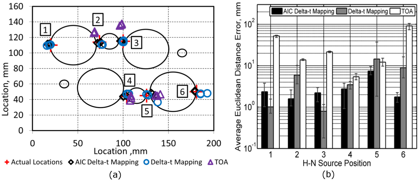
Fatigue specimen: (a) estimated H–N source location and (b) average error for each location.

Composite impact specimen

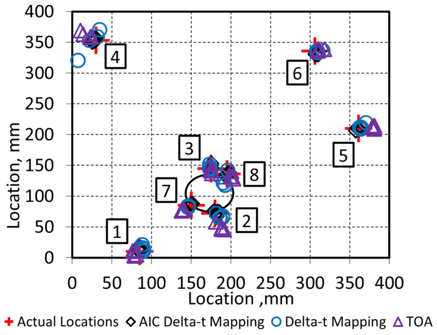
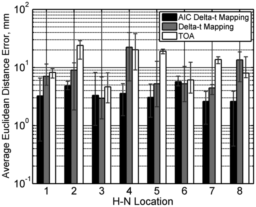
Figure 8 shows the located H–N source events and the average Euclidean distance error for each position for all the location methods. Again the Delta-t techniques are able to locate sensibly all H–N sources within the specimen’s geometric boundary when compared with just half of the positions with the TOA technique. The comparison of both Delta-t techniques shows that the improved AIC location algorithm is able to locate with a higher level of accuracy for 67% of the locations (positions 1, 2, 5 and 6), with improvements of 51, 1, 40 and 3 mm, respectively. The traditional Delta-t mapping technique shows an improvement of 0.22 and 7 mm, respectively, for locations 3 and 4. For location 4, the improvement of 7 mm in average error in the Delta-t mapping over the AIC Delta-t mapping requires further discussion. This difference in error is larger than the uncertainty in the measurements due to the sample rate and sensor face diameter which for this specimen were 1–1.5 and 4 mm, respectively, meaning another factor has contributed to this error. The reasons for this are most likely caused by the grid data for the AIC Delta-t technique. The training maps for the Delta-t between channels 1 and 2 and channels 3 and 4 in the proximity of (60,140) mm show a local peak and a change in gradient either side. This means that there are positions along these contours which are equal, meaning any variation in arrival time estimation could lead to two possible source locations and hence a larger error for this particular position. This is not the case for the Delta-t mapping contours where, due to the threshold crossing technique, the arrival time is less accurate. This therefore means the local variations are not present and results in a more accurate source estimation for this particular position. Another interesting result is the relatively high location inaccuracy for the Delta-t mapping for positions 1 and 5. For position 1, for each H–N source, the errors are 4, 4 and 168 mm. For location 5, similar results are observed with errors of 8, 8 and 113 mm from the source. The same training and H–N source AE data were used for both techniques showing the sensitivity in using arrival times calculated by threshold crossing for AE source location. This reinforces the use of the AIC Delta-t technique and shows the ability to confidently determine accurate source locations. In addition, no sensible source location was determined by the TOA algorithm for H–N location 1. The average Euclidean distance error for this position was 375 m and hence was not shown in the figure. The reasons for this large error are due to the H–N source position being located on the edge of the sensor array which is known to give large errors in TOA source location. Also, this particular H–N position is located close to a sensor, where the contours of Delta-t can change sharply resulting in small arrival time errors leading to large source location errors. These errors are further compounded by the fact that two of the source to sensors’ paths are on the fibre direction and hence the wave travels fastest in these directions, while the other two are off the fibre direction and hence travelling the slowest. The TOA algorithm is unable to account for the difference in wave speed for propagation angle and hence why there is significant error for this particular location.

Figure 8.

Composite impact specimen: (a) estimated H–N source location and (b) average error for each location.

Aluminium aircraft panel

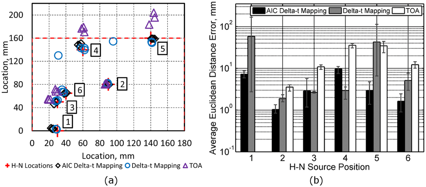
Figure 9 shows the estimated H–N source locations for all the source location techniques. All estimated H–N source positions were sensibly located within the boundary of the grid for this particular specimen. It is evident from the figure that the AIC Delta-t mapping technique shows a consistent average improvement of 9.3 and 5.1 mm over the TOA and Delta-t mapping techniques, respectively. The figure also shows that for H–N source positions in close proximity to the hole which have multiple source to sensor paths affected by this structural feature, the accuracy and precision of the estimated source locations are worse when compared with the AIC Delta-t technique. It also demonstrated the robustness of the AIC Delta-t mapping technique. Figure 10 shows the average Euclidean distance error for each H–N source location for all three location techniques. All source location estimations are located within 25 mm from the actual positions. For the AIC Delta-t mapping, all H–N source estimations are located within 10 mm from their actual position. While for the Delta-t mapping two of the eight locations have errors greater than 10 mm (positions 4 and 8). Also, at two positions (3 and 6), the Delta-t mapping technique has a minor improvement of the AIC mapping technique of 0.4 and 0.5 mm, respectively. The average Euclidean distance errors for all H–N locations are 3.6, 8.7 and 13 mm for the AIC Delta-t mapping, Delta-t mapping and TOA techniques, respectively. The potential source location errors due to the sample rate and sensor face diameter are 2.6 and 8 mm, respectively, for this specimen.

Figure 9.

Estimated H–N source location for aluminium aircraft panel.

Figure 10.

Average Euclidean distance error for each H–N source location.

Figure 11 presents a comparison of the traditional Delta-t mapping, which utilises a one-dimensional (1D) interpolation strategy, and the AIC Delta-t mapping using both the same 1D interpolation and a two-dimensional (2D) interpolation strategy. The three approaches are also compared across a range of grid resolutions. It is clear that the interpolation strategy has little effect on the performance of the Delta-t mapping approach with very similar accuracy observed for AIC Delta-t with both 1D and 2D interpolations. Considering that the Delta-t contour maps commonly change gradually and are generally smooth, this is relatively unsurprising. Hence, the observed improvements over the traditional Delta-t algorithm are predominantly related to the improved robustness in arrival time estimation. When considering the effect of grid resolution, the accuracy is only affected when the resolution reaches 100 mm, in this example, and even then not significantly. This also relates to the smoothness of the Delta-t contour maps, which here are relatively smooth and change gradually, meaning that interpolation works very effectively. If more complex structural features are present that cause local discontinuities within the contour maps, then a grid resolution is required that is suitable to capture the nature of these discontinuities. It should also be noted that should a local discontinuity in the contour maps not be suitably captured, it will only affect the location accuracy within that region and not globally.

Figure 11.

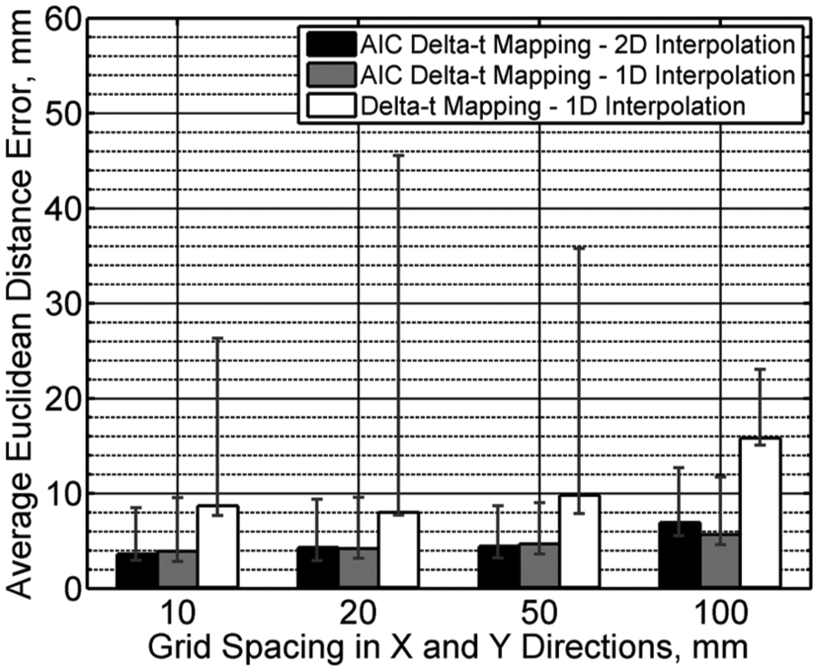
Average Euclidean distance error source location for all H–N locations for different grid resolutions.

Aerospace damage mechanism case studies

Two further case studies are presented to demonstrate the ability of the TOA and Delta-t mapping and the novel AIC Delta-t mapping to detect actual damage mechanisms which occur in the aerospace environment. Although validation of the technique using H–N sources is perfectly adequate, it does not give an indication of how the algorithms will perform when subjected to a test environment. Therefore, a comparison of the techniques is presented for detecting fatigue crack and impact events.

Aluminium fatigue study

Figure 12 shows the damage regions after the specimen had been subjected to 96,000 fatigue cycles. No damage was observed at the last visual inspection at 76,000 cycles. Closer visual observation after testing showed that a small fatigue crack initiated at the right-hand side thin section (Figure 12– solid arrow). This propagated a small distance before leading to a rapid failure of that section, which, in turn, caused a rapid failure of the left-hand side thin section (Figure 12– dashed arrow).

Figure 12.

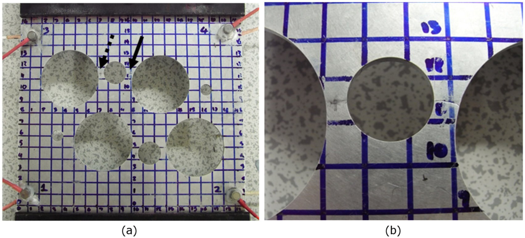
Resulting damage from the fatigue testing showing a) the damage locations and b) a close up image of the damage region.

Figure 13 shows the number of located events recorded throughout the fatigue test. The figure shows the last visual inspection (black dashed line) and the point at which the rate of located events increased at 88,000 cycles (red dashed line). This identifies the point at which significant damage occurred in the specimen. This suggests that the damage initiated and propagated within the final 8,000 cycles, and that approximately 15,000 events were located within this timeframe. Although not conclusive, this gives a clear indication when damage initiated and propagated in the structure, a clearer understanding of the deterioration of the structure, and shows the advantages of AE for SHM systems.

Figure 13.

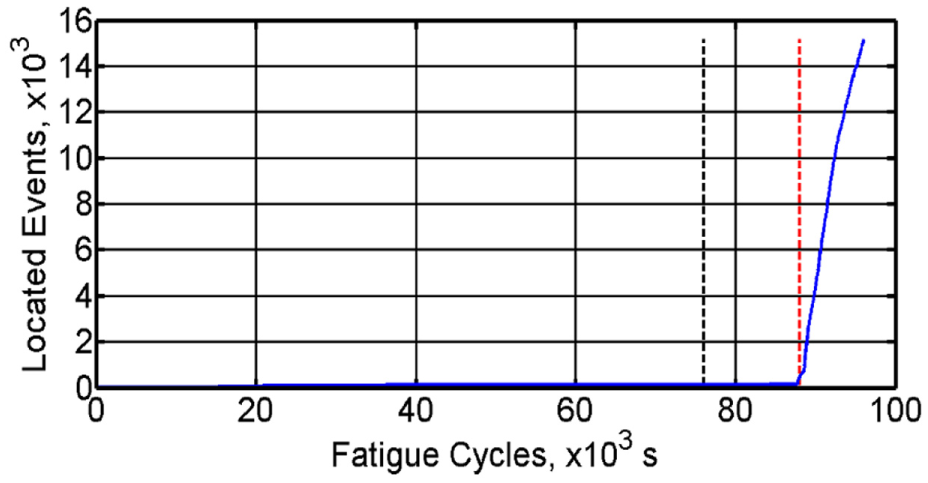
Events located throughout the fatigue testing.

Figure 14 illustrates the damage regions in the specimen as well as the results of spatially binned located events. The number of events that were located within each 5 × 5 mm spatial bin are shown. The results presented enable a comparison between the TOA, conventional and AIC Delta-t mapping techniques. The TOA results show three location groups, with the closest being approximately 15 mm away from the right-hand side thin section damage region. From these results, it would be difficult to conclude that damage had occurred in the specimen. The results for the Delta-t mapping improve on those of the TOA technique, with significantly higher numbers of located events occurring in the top half of the specimen. Again from these results, it would be difficult to confidently determine that damage had occurred in the structure. The spatial bin with the highest concentration of located events is at (100,135) mm and contains 381 events. Averaging the locations in this bin results in a Euclidean distance error of 24 mm. There are 50–100 events located on the right damage region; however, this event bin concentration also occurs frequently in the top half of the specimen, which adds further difficulty in confidently determining damage in the specimen. The AIC Delta-t mapping spatial binning results are very promising and due to the close grouping of located events show a clear indication that damage has occurred in the specimen. The results would allow for confident determination of an area of interest to investigate further. There are two areas of higher activity (greater than 250 events). The first and most active area contains 2117 events and is located 19 mm directly north of the right-hand damage region. A lower intensity of located events (217 events) occurs at the damage site. The relative size of this region of higher located events (2117 events) is not surprising as it is possible that the AE is being detected from plastic deformation and the damage region. The other area of higher activity is located at (55,130) mm and contains 381 events. This particular region could be from the left-hand side damage region. There are a variety of reasons why this area maybe mis-located; the first is that the higher AE activity of the right-hand side damage region could have masked signals from the left-hand side region, if the right-hand side damage region propagated all the way across this section before the left-hand section failed, causing alterations of the training grid resulting in erroneous locations. The final possible reason could be the rapid failure of this section, which was evident from the crack surfaces, arising in a short sudden release of AE activity. Although all three techniques have been unable to locate the damage on the left-hand thin section, the accuracy of the AIC Delta-t mapping technique would enable the user to have greater confidence that damage had occurred. It should also be stated that in total, both damage surfaces were 5 mm in length and the ability to accurately locate damage of this size is an achievement. Overall, the AIC Delta-t mapping shows a clear area of higher activity which could direct an operator to investigate the damage area further.

Figure 14.

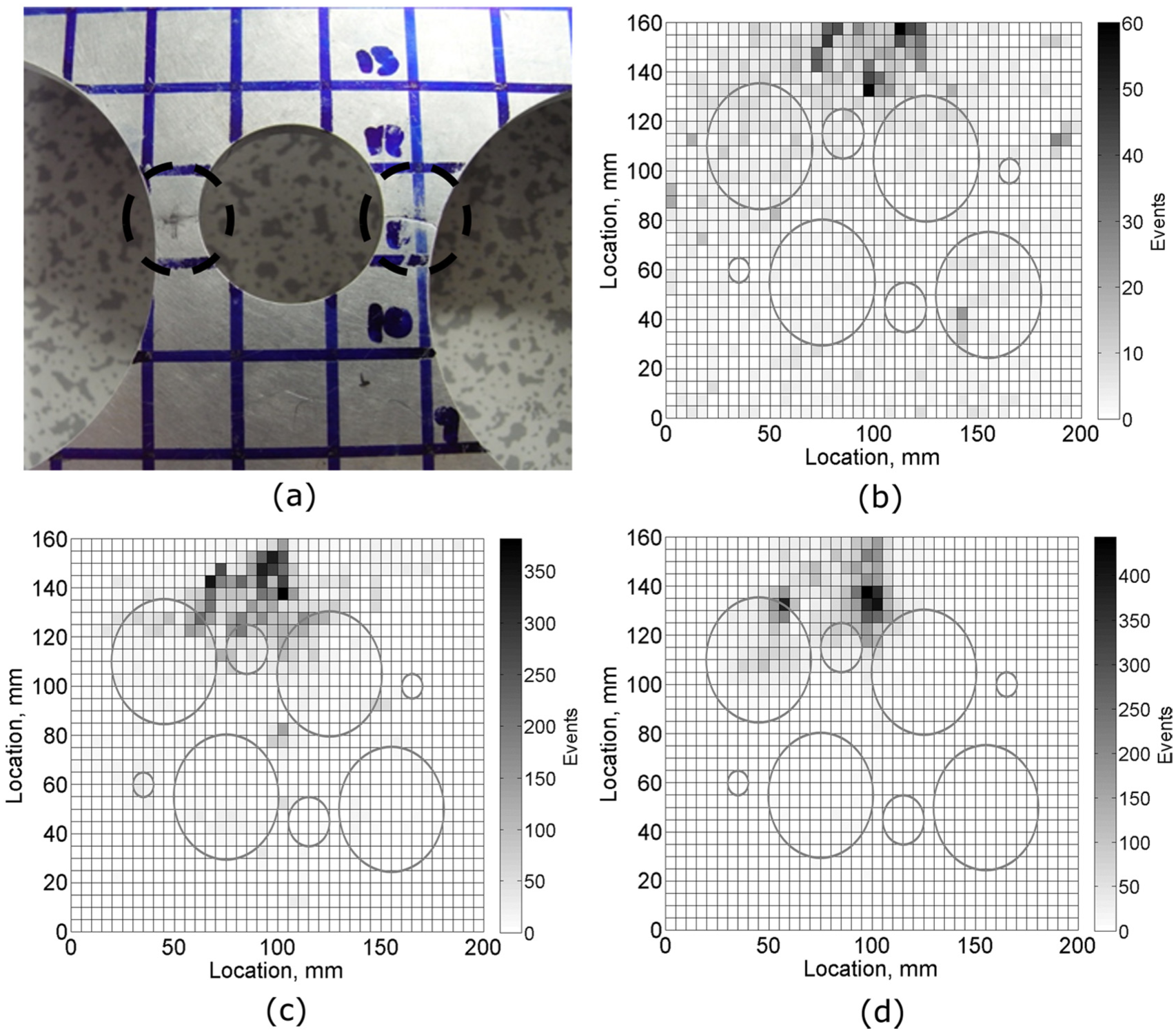
(a) Visual observation of the damage regions and the associated events’ spatial binning for all fatigue cycles for the (b) TOA, (c) Delta-t and (d) AIC Delta-t mapping.

Figure 15 shows the results of energy spatial binning where individual bins represent the energy summation of the first hit sensor in the event. The energy approach can be another useful tool for determining significant AE activity. The figure also shows the average Euclidean distance error for located events in spatial bins with energy levels greater than 7.2 × 10⁷ aJ. The location events within these bins were averaged to gain a representative evaluation of the accuracy of each technique. In addition, the figure shows the number of events contained within these higher energy spatial bins. The results for the TOA technique show a region of higher energy located 20.2 mm away from the right-hand side damage region; the total AE energy recorded is 3.99 × 10⁸ aJ from 102 events. The results for Delta-t mapping again show one specific region of higher AE activity; this area on average is located 4.19 mm away from the damage region and contains a total energy of 3.51 × 10⁸ aJ from 213 events. Finally, the results for the AIC Delta-t mapping show that it is the only technique where the significant energy bins are located at the damage region. The higher AE activity region is located within an average error of 3.42 mm from the damage region and totals a region of 3.91 × 10⁸ aJ and contains 410 events. Both the traditional and AIC Delta-t mapping technique show an improvement over the TOA technique where a reduction in the average error of 15.97 and 16.74 mm was observed, respectively. The comparison of the traditional and AIC Delta-t mapping technique shows similar performance in the average error when detecting aluminium fatigue damage. However, a significant improvement is that the AIC Delta-t technique has located a further 197 events when compared with traditional technique. From a statistical approach, this can further improve the confidence of damage location, showing that the AIC Delta-t mapping is able to locate lower energy events more consistently than the Delta-t mapping technique. Therefore, this has the potential to provide an earlier indication of the damage presence.

Figure 15.

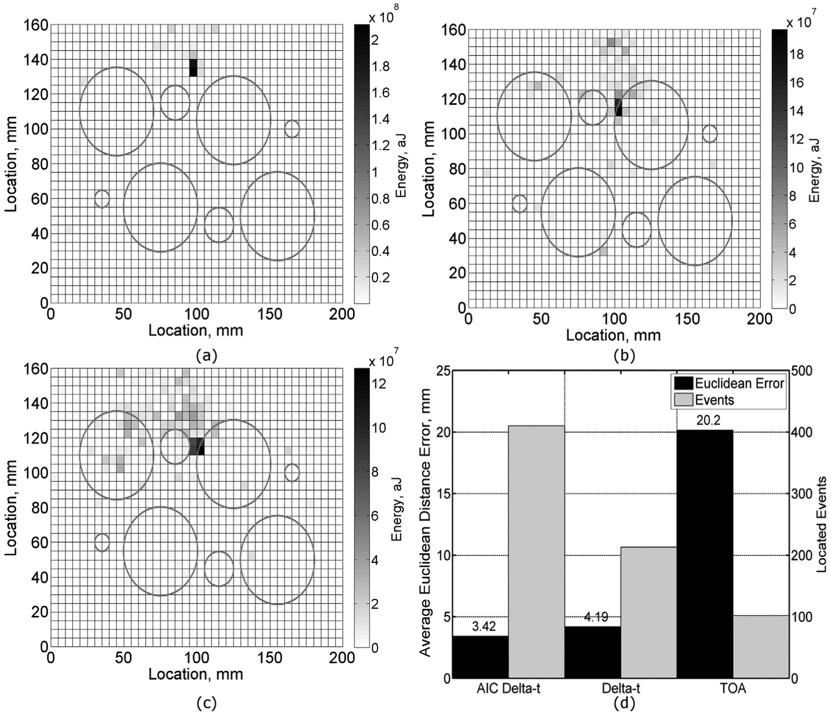
AE energy spatial binning for all fatigue cycles for the (a) TOA, (b) Delta-t and (c) AIC Delta-t mapping and (d) the Euclidean distance area for spatial bins above the energy threshold.

Composite impact specimen

Ultrasonic C-scans were performed pre and post impact testing; the results for the pre-impact C-scan showed that there was no manufacturing damage in the panel. Figure 16 shows the C-scan results for the specimen after it was subjected to four impacts with respective impact energies of 3, 4, 5 and 5 J. The figure clearly shows an area of delamination at the impact location, which had an approximate size of 188 mm² using ‘−6 dB drop method’.^51,52 The other higher attenuation areas correspond to the four sensors. Figure 17 shows the results of the TOA, Delta-t and AIC Delta-t mapping locations for the impact events overlaid on the C-scan image. The TOA technique located all four impact events; however, none was located within the delamination area. The Delta-t technique located three of the four impacts and was unable to locate impact 1. The TOA technique located impact 1 at (−362,22) mm; this large error has arisen due to inaccurate arrival time estimation using the threshold crossing technique, and therefore, erroneous Delta-t is used in the TOA algorithm. This also effects the calculation of the source position using the Delta-t mapping technique, meaning the impact event Delta-t’s fall outside those contained in the training grids, and therefore, no source position can be determined. The impact locations for the AIC Delta-t mapping technique are extremely promising, locating all four impacts within the damage area. Figure 18 shows the Euclidean distance errors calculated for each impact. Comparing all three techniques, the TOA technique’s largest and smallest location errors were 404 and 19 mm, respectively, while for the Delta-t mapping these values were 39 and 5 mm. The most accurate technique was the AIC Delta-t mapping with the maximum and minimum errors of 5 and 2.5 mm, respectively. The average Euclidean distance errors for all the located impact events for the TOA, traditional Delta-t and AIC Delta-t mapping were 124.7, 18.9 and 3.3 mm, respectively. Again these results show the performance enhancement of the AIC Delta-t mapping for locating impact events with significant improvements in the accuracy and confidence that all impacts will be located. This is increasingly important as impact events are one off events. It is noted that despite the clamping frames sitting between the impact site and the sensor positions, they do not appear to have a detrimental effect on the location accuracy (Figure 18). The small width of the frames (20 mm) and the dry interface (i.e. they are not acoustically coupled to the sample) mean that their effect on propagation is minimal. Consideration of frequency content and attenuation of the recorded waves may reveal some changes, but the concern here is the time of flight (ToF) from source to sensor which appears to have remained unaffected.

Figure 16.

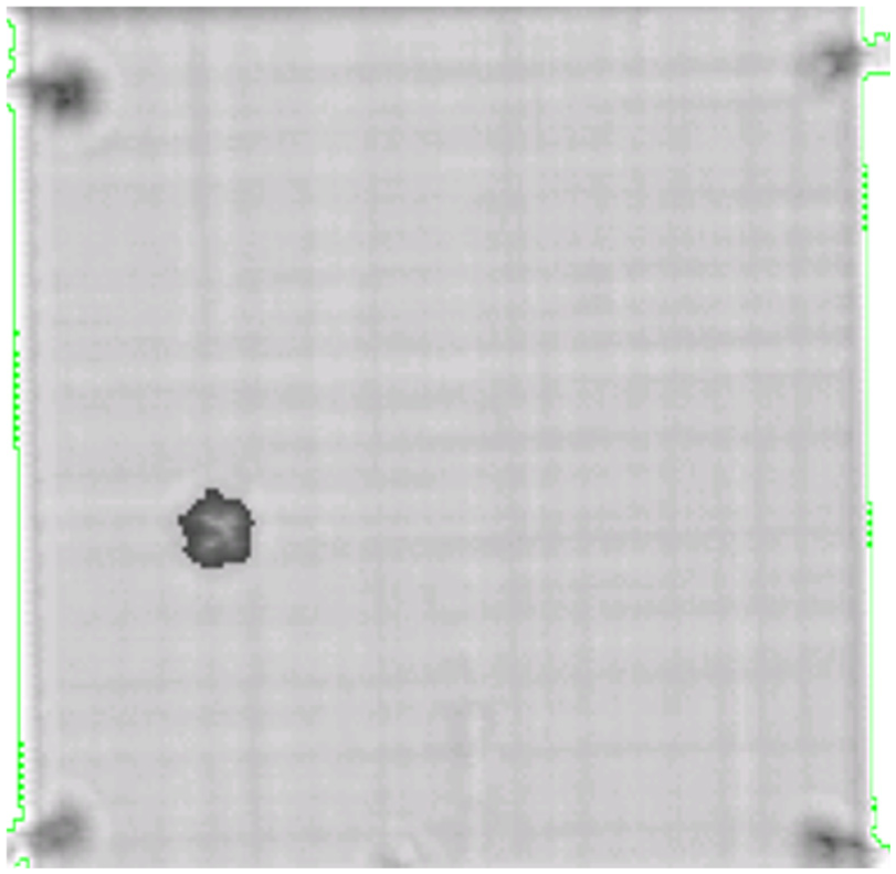
Ultrasonic C-scan of composite impact specimen.

Figure 17.

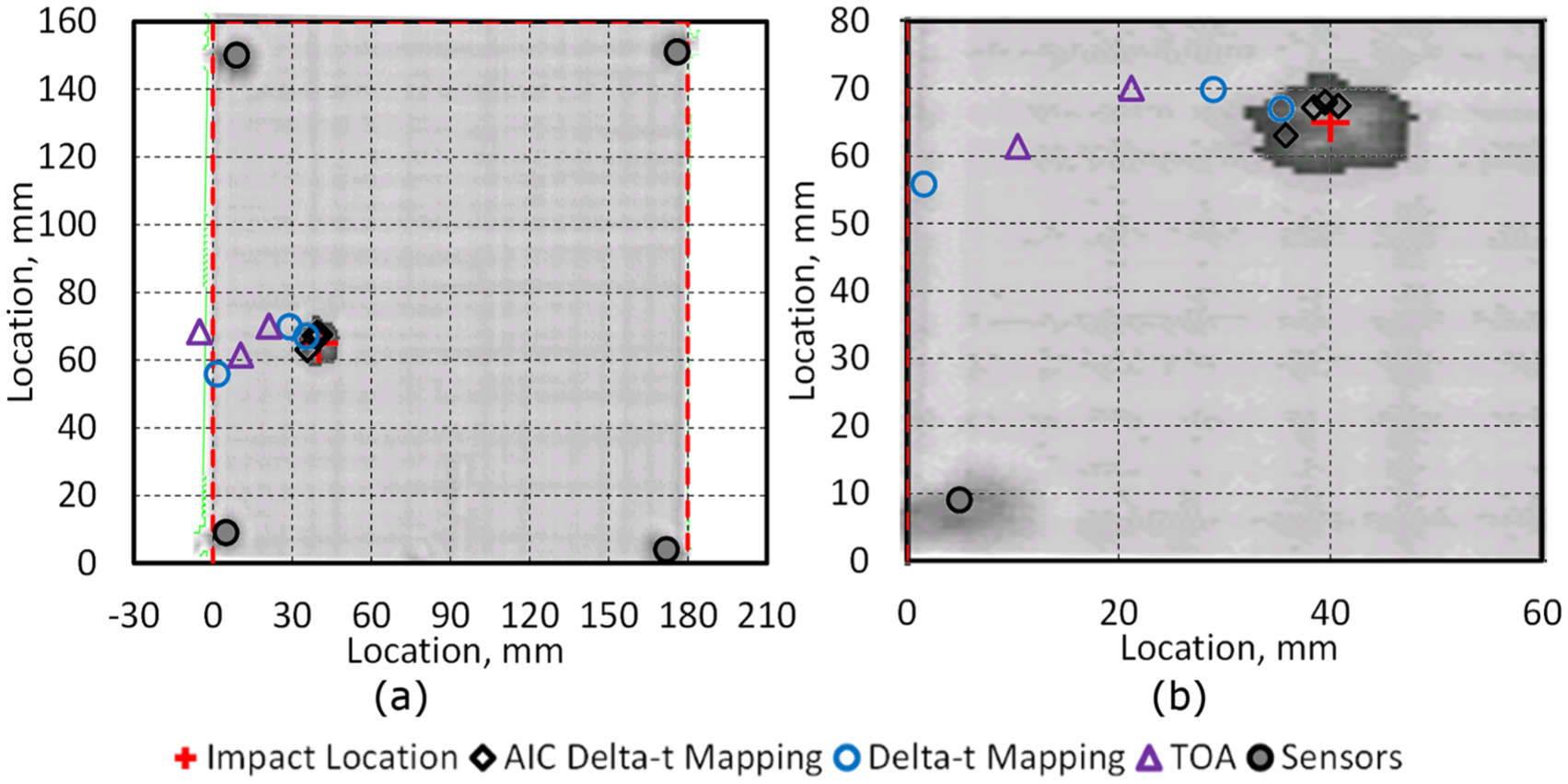
Composite impact specimen estimated H–N source locations showing the a) identified area of interest and b) a close up of the damage region.

Figure 18.

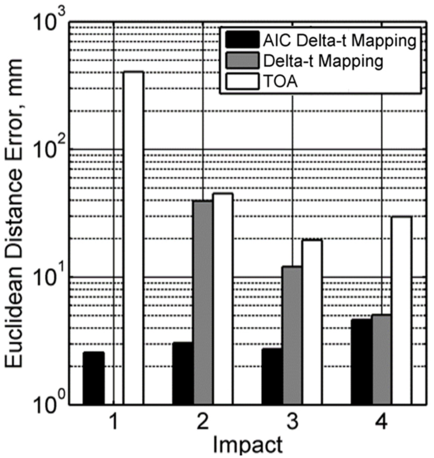
Euclidean distance error for each impact event.

Results summary

Table 2 shows the summary of the average Euclidean source location error for all the investigations undertaken for both specimens. For locating H–N sources on the aluminium specimen, the average Euclidean source location error was 32.6, 5.8 and 3 mm for the TOA, traditional and AIC Delta-t mapping techniques, respectively. For locating fatigue damage, the average errors were 20.2 mm (TOA), 4.2 mm (Delta-t) and 3.4 mm (AIC Delta-t). In addition, the AIC Delta-t technique was able to locate a further 197 and 308 events in the spatial bins with an accumulated energy greater than 7.2 × 10⁷ aJ. For locating H–N sources on the composite specimen, the average error was 19.3 mm (TOA), 18.9 mm (Delta-t) and 4.2 mm (AIC Delta-t). Furthermore, for locating impact events, the average errors were 124.7 mm (TOA), 18.9 mm (Delta-t) and 3.3 mm (AIC Delta-t). Finally, the results of a larger grid (400 × 400 mm) for locating H–N sources on an aircraft panel showed the average errors of 13.0 mm (TOA), 8.7 mm (Delta-t) and 3.6 mm (AIC Delta-t) mapping. Overall, AIC Delta-t mapping shows a reduction in error irrespective of the material or source type when compared with the other two techniques and excellent accuracy with average errors less than 4.2 mm, which was not achieved with the other techniques. In all the presented examples, a single set of training data were captured and used to locate damage from subsequent testing. The question still remains as to how much damage or degradation a structure can sustain before the training data become invalid. If damage occurs at a localised site, such as an impact event on a composite panel, then this damage will only affect subsequent location calculations if it interrupts the shortest path from a new source to any sensors and hence changes the ToF and therefore Delta-t values. For example, in the case of the composite impact tests above, multiple impacts were performed at the same location and all accurately located, without update to the training data. However, in this example, the damage all occurred at the same position and wave paths propagated from the damage site out to sensors, uninterrupted, hence accuracy was maintained. Had damage occurred at a different position and the resulting waves had to travel through a previous damage site, then a reduction in accuracy would be expected. The extent of this change will depend on both the position of the existing and the new damage and also the type and extent of damage present.

Table 2.

Summary of the average Euclidean error in source location.

		Average Euclidean source location error (mm)
		TOA	Delta-t	AIC Delta-t
Aluminium specimen	H–N sources	32.6	5.8	3.0
Aluminium specimen	Fatigue damage	20.2	4.2	3.4
Composite specimen	H–N sources	19.3	18.9	4.2
Composite specimen	Impact events	124.7	18.9^a	3.3
Aircraft panel	H–N sources	13.0	8.7	3.6

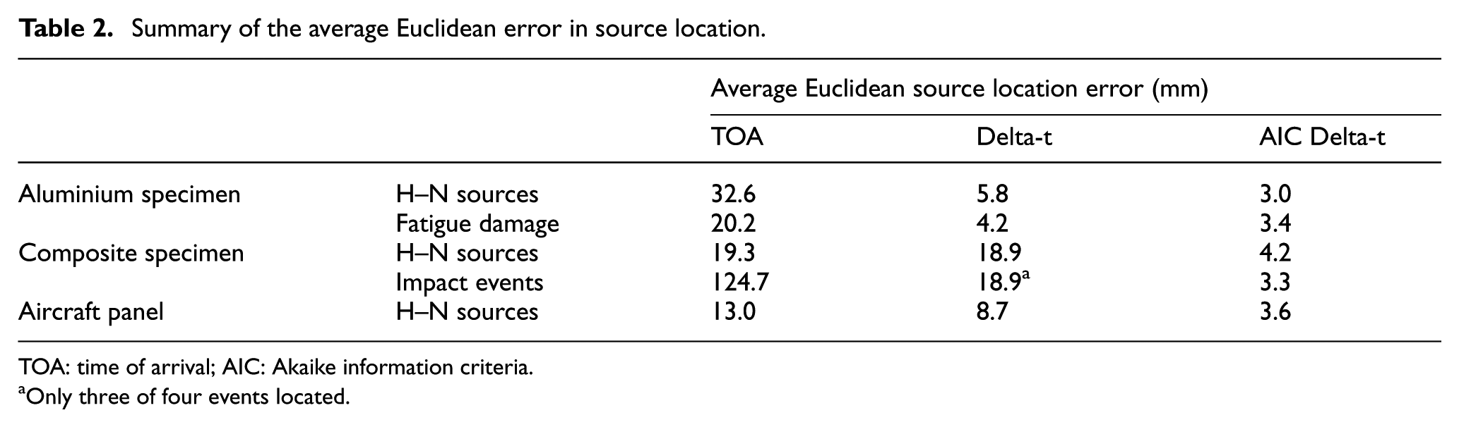
TOA: time of arrival; AIC: Akaike information criteria.

Only three of four events located.

Conclusion

TOA, Delta-t and the novel AIC Delta-t mapping techniques were used to locate H–N sources, fatigue damage in aluminium and impact events in composite panels. The AIC Delta-t technique was able to consistently show accuracy improvements when compared with the TOA and the Delta-t mapping when locating H–N sources in aluminium and composite specimens. The ability of all three location techniques to detect real damage mechanisms, which could be prevalent when using an SHM system in reality, was assessed. For locating fatigue damage, the AIC Delta-t mapping technique produced results where a user could confidently determine an area of interest. Increasing the confidence damage could be detected and shows that AIC Delta-t mapping can accurately detect lower energy events. Finally, the results for locating impacts showed the AIC Delta-t mapping technique located all four impacts with the highest level of accuracy, further demonstrating the robustness of the AIC Delta-t mapping technique for located different damage mechanisms. Overall, the combination of the Delta-t mapping technique with an AIC picker is able to provide accurate location and showed significant improvements over the conventional TOA and Delta-t mapping techniques. The use of the AIC Delta-t mapping for locating damage in an SHM system would allow confident and more probable detection of damage irrespective of the threshold used. Often damage location is the first step in any SHM system; this needs to be achieved with accuracy and confidence so that any other technique used, such as classification, can determine the nature of deterioration. The AIC Delta-t mapping technique offers a very credible method of achieving this and in reality could lead to a greater confidence in SHM systems.

Footnotes

Declaration of Conflicting Interests

The author(s) declared no potential conflicts of interest with respect to the research, authorship and/or publication of this article.

Funding

The author(s) disclosed receipt of the following financial support for the research, authorship, and/or publication of this article: This work was supported by Innovate UK (grant number 100444).

References

Beral

Speckmann

. Structural health monitoring (SHM) for aircraft structures: a challenge for system developers and aircraft manufacturers. In: Chang

(ed.) Structural health monitoring 2003: from diagnostics & prognostics to structural health management: proceedings of the 4th international workshop on structural health monitoring. Lancaster, PA: DEStech Publications, 2003, pp. 12–28.

Kapoor

Boller

Worden

. Prospective applications for SHM on commercial aircraft. In: Chang

(ed.) Structural health monitoring 2009: from system integration to autonomous systems: proceedings of the 7th international workshop on structural health monitoring. Lancaster, PA: DEStech Publications, 2009, pp. 223–230.

Chang

Markmiller

JFC

. A new look in design of intelligent structures with SHM. In: Structural health monitoring 2006: proceedings of the third European workshop on structural health monitoring, Granada, 5–7 July 2006, pp. 5–20. Lancaster, PA: DEStech Publications.

Miller

Hill

EvK

Moore

PO.

Nondestructive testing handbook, third edition: volume 6: acoustic emission testing. Columbus, OH: ASNT, 2005.

Mostafapour

Davoodi

Ghareaghaji

Acoustic emission source location in plates using wavelet analysis and cross time frequency spectrum. Ultrasonics 2014; 54: 2055–2062.

Paget

Atherton

O’Brien

. Triangulation algorithm for damage location in aeronautical composites structures. In: Chang

Flynn

Todd

Wilcox

. Maximum-likelihood estimation of damage location in guided-wave structural health monitoring. P Roy Soc A: Math Phy 2011; 467: 2575–2596.

Ward

Croxford

Paget

Passive impact localisation for the structural health monitoring of new airframe materials. J Phys Conf 2013; 457: 1–11.

Koabaz

Hajzargarbashi

Kundu

. Locating the acoustic source in an anisotropic plate. Struct Health Monit 2011; 11: 315–323.

10.

Kundu

Das

Martin

. Locating point of impact in anisotropic fiber reinforced composite plates. Ultrasonics 2008; 48: 193–201.

11.

Improving source location accuracy of acoustic emission in complicated structures. J Nondest Eval 2009; 28: 1–8.

12.

Ciampa

Meo

A new algorithm for acoustic emission localization and flexural group velocity determination in anisotropic structures. Compos Part A: Appl S 2010; 41: 1777–1786.

13.

Ciampa

Meo

Baram

Impact localization in composite structures of arbitrary cross section. Struct Health Monit 2012; 11: 643–655.

14.

Aljets

Chong

Wilcox

. Acoustic emission source location in plate-like structures using a closely arranged triangular sensor array. J Acoust Emiss 2010; 28: 85–98.

15.

Surgeon

Wevers

One sensor linear location of acoustic emission events using plate wave theories. Mat Sci Eng A: Struct 1999; 265: 254–261.

16.

Matt

Lanza di Scalea

Macro-fiber composite piezoelectric rosettes for acoustic source location in complex structures. Smart Mater Struct 2007; 16: 1489–1499.

17.

Kundu

Nakatani

Takeda

Acoustic source localization in anisotropic plates. Ultrasonics 2012; 52: 740–746.

18.

Kundu

Yang

Nakatani

. A two-step hybrid technique for accurately localizing acoustic source in anisotropic structures without knowing their material properties. Ultrasonics 2015; 56: 271–278.

19.

Grosse

. Acoustic emission localization methods for large structures based on beamforming and array techniques. In: 7th International symposium on nondestructive testing in civil engineering, Nantes, 30 June–3 July 2009.

20.

Pan

Liu

. Near-field beamforming analysis for acoustic emission source localization. Ultrasonics 2012; 52: 587–592.

21.

Xiao

Pan

. A novel acoustic emission beamforming method with two uniform linear arrays on plate-like structures. Ultrasonics 2014; 54: 737–745.

22.

Schumacher

Straub

Higgins

Towards a probabilistic acoustic emission source location algorithm: a Bayesian approach. J Sound Vib 2012; 331: 4233–4245.

23.

Zarate

Pollock

Momeni

. Structural health monitoring of liquid-filled tanks: a Bayesian approach for location of acoustic emission sources. Smart Mater Struct 2015; 24: 1–10.

24.

Yan

Tang

A Bayesian approach for localization of acoustic emission source in plate-like structures. Math Probl Eng 2015; 2015: 1–14.

25.

Niri

Farhidzadeh

Salamone

Adaptive multisensor data fusion for acoustic emission source localization in noisy environment. Struct Health Monit 2012; 12: 59–77.

26.

Niri

Farhidzadeh

Salamone

Nonlinear Kalman filtering for acoustic emission source localization in anisotropic panels. Ultrasonics 2014; 54: 486–501.

27.

Julier

Uhlmann

JK.

New extension of the Kalman filter to nonlinear systems. Proc SPIE 1997; 3068: 182–193.

28.

St-Pierre

Gringas

. Comparison between the unscented Kalman filter and the extended Kalman filter for the position estimation module of an integrated navigation information system. In: Proceedings of IEEE intelligent vehicle symposium, Parma, 14–17 June 2004, pp. 831–835. New York: IEEE.

29.

Niri

Farhidzadeh

Salamone

Determination of the probability zone for acoustic emission source location in cylindrical shell structures. Mech Syst Signal Pr 2015; 60–61: 971–985.

30.

Scholey

Wilcox

Wisnom

. A generic technique for acoustic emission source location. J Acoust Emiss 2009; 27: 291–298.

31.

Hensman

Mills

Pierce

. Locating acoustic emission sources in complex structures using Gaussian processes. Mech Syst Signal Pr 2010; 24: 211–223.

32.

Ziola

Gorman

MR.

Source location in thin plates using cross-correlation. J Acoust Soc Am 1991; 901: 2551–2556.

33.

Jeong

Analysis of plate wave propagation in anisotropic laminates using wavelet transform. NDT&E Int 2001; 34: 185–190.

34.

Jeong

Jang

YS.

Fracture source location in thin plates using the wavelet transform of dispersive waves. IEEE T Ultrason Ferr 2000; 47: 612–619.

35.

Hsu

Breckenbridge

FR.

Characterisation and calibration of acoustic emission sensors. Mater Eval 1981; 39: 60–68.

36.

Hamstad

O’Gallagher

Gary

A wavelet transform applied to acoustic emission signals: part 2: source location. J Acoust Emiss 2002; 20: 62–82.

37.

Ding

Reuben

Steel

JA.

A new method for waveform analysis for estimating AE wave arrival times using wavelet decomposition. NDT&E Int 2004; 37: 279–290.

38.

Shehadeh

Steel

Reuben

RL.

Acoustic emission source location for steel pipe and pipeline applications: the role of arrival time estimation. Proc IMechE Part E: J Process 2006; 220: 121–133.

39.

Lokajicek

Kilma

A first arrival identification system of acoustic emission signals by means of a high-order statistics approach. Meas Sci Technol 2006; 17: 2461–2466.

40.

Baer

Kradolfer

An automatic phase picker for local and teleseismic events. B Seismol Soc Am 1987; 77: 1437–1445.

41.

Akaike

Markovian representation of stochastic processes and its application to the analysis of autoregressive moving average processes. Ann I Stat Math 1974; 26: 363–387.

42.

Kitagawa

Akaike

A procedure for the modeling of non-stationary time series. Ann I Stat Math 1978; 30: 351–363.

43.

Hinkley

DV.

Inference about the change-point for cumulative sum tests. Biometrika 1971; 58: 509–523.

44.

Grosse

Winpecker version 1.2: instruction manual. Stuttgart: University of Stuttgart, 2000.

45.

Kurz

Grosse

Reinhardt

HW.

Strategies for reliable automatic onset time picking of acoustic emissions and of ultrasound signals in concrete. Ultrasonics 2005; 2005: 538–546.

46.

Carpinteri

Lacidogna

. Reliable onset time determination and source location of acoustic emissions in concrete structures. Cement Concrete Comp 2012; 34: 529–537.

47.

Sedlak

Hirose

Enoki

Acoustic emission localization in thin multi-layer plates using first-arrival determination. Mech Syst Signal Pr 2013; 36: 636–649.

48.

Sedlak

Hirose

Khan

. New automatic localization technique of acoustic emission signals in thin metal plates. Ultrasonics 2009; 49: 254–462.

49.

Baxter

Pullin

Holford

. Delta T source location for acoustic emission. Mech Syst Signal Pr 2007; 21: 1512–1520.

50.

Eaton

Pullin

Holford

KM.

Acoustic emission source location in composite materials using delta T mapping. Compos Part A: Appl S 2012; 43: 856–863.

51.

Broughton

Sims

Lodeiro

MJ.

Overview of DTI-funded programme on ‘Standardised procedures for ultrasonic inspection of polymer matrix composites’. Insight: Non-Dest Test Cond Monit 1998; 40: 8–11.

52.

Smith

Jones

Willsher

. Diffraction and shadowing errors in −6 dB defect sizing of delaminations in composites. Insight: Non-Dest Test Cond Monit 1998; 40: 44–49.

Improved acoustic emission source location during fatigue and impact events in metallic and composite structures

Abstract

Keywords

Introduction

AE source location

Onset picking

Delta-t mapping

Improved AIC Delta-t mapping

Experimental procedure

Aluminium fatigue specimen

Composite impact specimen

Aluminium aircraft panel

Experimental results and discussion

H–N source investigations

Complex fatigue specimen

Composite impact specimen

Aluminium aircraft panel

Aerospace damage mechanism case studies

Aluminium fatigue study

Composite impact specimen

Results summary

Conclusion

Footnotes

Declaration of Conflicting Interests

Funding

References