Frequentist and Bayesian approaches to data analysis: Evaluation and estimation

Abstract

Statistical thinking is essential to understanding the nature of scientific results as a consumer. Statistical thinking also facilitates thinking like a scientist. Instead of emphasizing a “correct” procedure for data analysis and its outcome, statistical thinking focuses on the process of data analysis. This article reviews frequentist and Bayesian approaches such that teachers can promote less well-known statistical perspectives to encourage statistical thinking. Within the frequentist and Bayesian approaches, we highlight important distinctions between statistical evaluation versus estimation using an example on the facial feedback hypothesis. We first introduce some elementary statistical concepts, which are then illustrated with simulated data. Finally, we demonstrate how these approaches are applied to empirical data obtained from a Registered Replication Report. Data and R code for the example are provided as supplementary teaching material. We conclude with a discussion of key learning outcomes centred on promoting statistical thinking.

Research in statistics education advocates statistical thinking that is supported by the Guidelines for Assessment and Instruction in Statistics Education College Report (GAISE College Report American Statistical Association Revision Committee, 2016). Statistical thinking promotes the selection of appropriate models over applying a “correct” procedure to the data (Doerr & English, 2003; Wild & Pfannkuch, 1999). Statistical thinking discourages teaching students from following “recipes” by shifting focus to being a data detective (Rodgers, 2010; Schoenfeld, 1998; Tukey, 1969), reflecting the process of adjudicating new information, where the evidence is examined or evaluated with respect to extant hypotheses, expectations, or beliefs. Teaching statistical thinking is one way to address the perception of a replication crisis, stemming from ritualizing the application of statistical tests in a procedural fashion (Gigerenzer, 2018; Tukey, 1969).

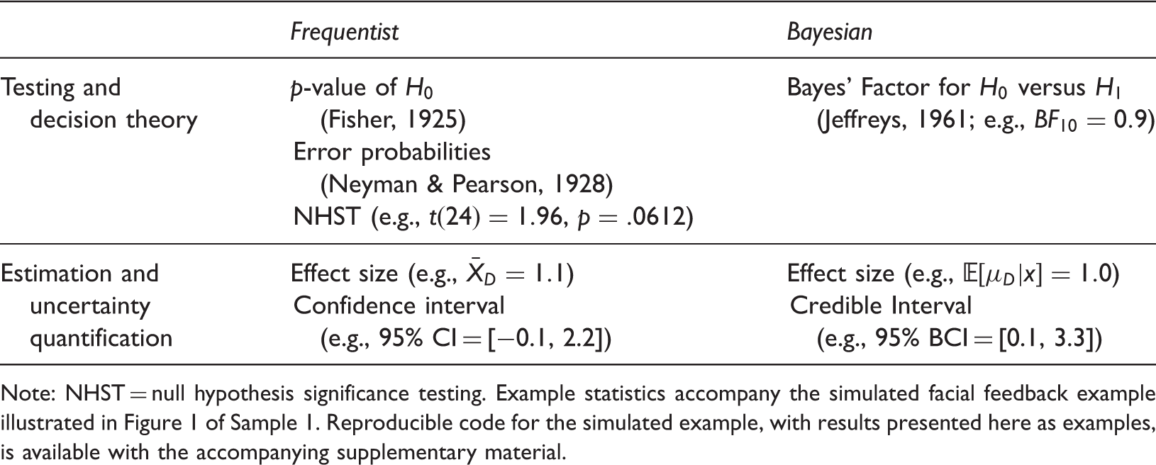
This paper presents a general framework that organizes alternative approaches and perspectives to statistics employed in psychological science (i.e., frequentist versus Bayesian and evaluation-based versus estimation-based; Table 1; cf. Jeon & De Boeck, 2017; Kruschke & Liddell, 2018). Our review of this taxonomy serves as a cornerstone for teachers in psychology to promote less well-known statistical perspectives. Familiarity with these alternatives to analysing and making sense of the same data from different perspectives is a starting point to statistical thinking.

Table 1.

Taxonomy of alternative statistical approaches in psychological science.

	Frequentist	Bayesian
Testing and decision theory	p-value of H0 (Fisher, 1925) Error probabilities (Neyman & Pearson, 1928) NHST (e.g., $t(24)=1.96$ , $p=.0612$ )	Bayes’ Factor for H0 versus H1 (Jeffreys, 1961; e.g., ${\mathit{BF}}_{10}=0.9$ )
Estimation and uncertainty quantification	Effect size (e.g., ${\overline{X}}_D=1.1$ ) Confidence interval (e.g., 95% CI = [−0.1, 2.2])	Effect size (e.g., $\mathbb{E}[{\mu }_D|x]=1.0$ ) Credible Interval (e.g., 95% BCI = [0.1, 3.3])

Note: NHST = null hypothesis significance testing. Example statistics accompany the simulated facial feedback example illustrated in Figure 1 of Sample 1. Reproducible code for the simulated example, with results presented here as examples, is available with the accompanying supplementary material.

As a motivating example, consider the facial feedback hypothesis, which posits that people’s affective perceptions are influenced by their own facial expressions (e.g., smiling or pouting), even when these expressions are not due to an emotional experience. In a famous experiment, Study 1 in Strack, Martin, and Stepper (1988) had participants hold a pen with their lips forming a “pout” versus holding a pen with their teeth forming a “smile” while rating cartoons with the pen in their mouths. Cartoons were rated on whether they were 0 = not at all funny to 9 = very funny on a 10-point Likert-type scale. In a between-subjects design, participants endorsed higher ratings in the smile condition ( ${\overline{X}}_{\text{smile}}$  = 5.14) compared with the pout condition ( ${\overline{X}}_{\text{pout}}=4.32$ ), or a ${\overline{X}}_D=.82$ unit difference, which was taken as evidence in support of the facial feedback hypothesis.

Concepts underlying evaluation and estimation

Does facial posture influence ratings of amusement or, more critically, a person’s mood? To answer this question, we need to analyse data. Specifically, we need to quantify the extent to which our data support our hypotheses (i.e., perform a statistical test to evaluate the extent to which the data stem from a hypothesis), or we need to estimate the effect size or parameters of a model that represents the effect of facial posture on mood. First, we need to decide if we will take an evaluative or an estimation approach, and then we need to decide if we will take a frequentist or a Bayesian approach (see Table 1).

We should note at this point that the standard null hypothesis significance testing approach, which is current practice in psychology and the social sciences, falls into none of these approaches. We will discuss this issue in the Evaluation of hypotheses section next.

Evaluation of hypotheses

Evaluation ¹ of a hypothesis can be done from either a frequentist or a Bayesian perspective. The frequentist approaches can be categorized according to the Fisherian or Neyman-Personian approaches. The Bayesian perspective considers the probability of the null hypothesis as well as the relative odds of different hypotheses based on the observed data.

Fisherian approach

Fisher’s (1934) approach starts with a null hypothesis; e.g., H₀: no effect of facial posture $({\mu }_D=0$ ), where ${\mu }_D$ is the population mean difference. The null hypothesis is always formulated as an absence of an effect, so the population mean difference between the smile and pout conditions is equal to zero. Assuming H₀ is true we can compute the probability of observing a mean difference as large as ${\overline{X}}_D=.82$ and over repeated experiments, a p-value: P (observed mean difference ≥ .82 $;H_0$ : no effect of facial posture). ² A large p-value (say, .9100) implies that the observed mean difference is consistent with H₀ whereas a small p-value (say, .0012) implies the opposite. Fisherian evaluation examines the probability of the observed data (and more extreme values) assuming that H₀ is true (i.e., inductive inference; Lehmann, 1993), but does not involve rejecting H₀ (e.g., deciding that, in contrast to H₀, facial posture has an effect on mood). Instead, the p-value quantifies how well H₀ accounts for the data.

Neyman-Pearson decision theory

Decisions are required to inform behaviour, which is the basis of Neyman-Pearson (N-P) testing (i.e., inductive behaviour; Lehmann, 1993). To improve on Fisher’s procedures, N-P introduced the idea of an alternative hypothesis H₁. Suppose that a teacher, aware of the facial feedback hypothesis, plans to conduct his own experiment to help him decide whether to have his/her students put their pencils in their teeth to start the day for the rest of the school year. ³

Recall that H₀: no effect of facial posture on mood ( ${\mu }_D=0$ ), and suppose that past research suggests that the mean increase in amusement from holding a pencil in one’s teeth is at least 1.0 (see above). Under N-P testing, we can then establish an alternative hypothesis H₁: facial posture affects mood, with an effect size of ${\mu }_D=1.0$ . The teacher might waste time having his students begin the day by putting pencils in their mouths when there is no effect of facial posture on mood (i.e., rejecting H₀ when H₀ is true, a Type I error). Alternatively, he could fail to take advantage of a simple strategy to aid in classroom management when there is an effect of facial posture on mood (i.e., accepting H₀ when H₁ is true, a Type II error).

Part of the teacher’s decision must involve an evaluation of the relative costs of Type I and Type II errors. Let the probabilities of Type I and Type II errors be written as α and β, respectively. These probabilities are determined by the values of ${\mu }_D$ provided by the null and alternative hypotheses (the effect size) and the number of students he will measure in the experiment (the sample size, which determines the variance of the sampling distributions of the mean difference between the smile and pout conditions). Because making mistakes is costly, he wants to keep both α and β small.

After choosing acceptable α and β (say, .01 and .20, respectively) the teacher must determine the sample size that maintains these error rates. The error rates (and, potentially, the relative costs of each type of error) determine the critical value of ${\overline{X}}_D$ for which he will decide to either perform or forgo the daily activity. Equivalently, he could make the decision on the basis of the p-value of ${\mu }_D$ , and accept H₀ when p > .01 or accept H₁ when p < .01.

It is important to recognize that the decision to perform the activity or not is a dichotomization of a continuous quantity (the p-value) and that rejecting a hypothesis does not make the hypothesis false. Conversely, accepting a hypothesis does not make the hypothesis true. When the teacher accepts H₁ because the p-value of ${\overline{X}}_D$ was less than α, and decides that all his students will begin the day by holding their pencils in their teeth, he knows that students’ mood may not improve 1 out of 100 days $(\alpha =.01)$ . When the teacher accepts H₀ and decides not to have the students hold pencils in their teeth, he knows that the students might have improved their mood by doing so 80 out of 100 days ( $\beta =.20$ ). The teacher is not making an inference about mood changes due to facial posture; he is making a decision about whether he should implement the activity for the rest of the year.

Null hypothesis significance testing

The difference between Fisherian and N-P statistical evaluation dwells in use of the alternative hypothesis and the distinction between inductive inference and statistical decision-making. The confusion between the approaches has led to the current ritual called null hypothesis significance testing (NHST; Gigerenzer, 2004). Fisher was concerned with quantifying discrepancies between data and the null hypothesis without consideration of alternatives to the null. By contrast, N-P were concerned with controlling errors in statistical decisions. In N-P testing, alternatives to the null are proposed and these alternatives open the way for the concepts of Type I and Type II errors and consideration of sample size.

NHST borrows the alternative hypothesis concept from the N-P approach and the significance evaluation from the Fisherian approach. With these two notions we arrive at a ritual in which a p-value is computed based on long-run (frequentist) notions of sampling variability. The goal is to reject H₀ using the p-value and by so doing make a claim of the truth of the alternative hypothesis.

The NHST procedure is what Abelson (1995) called “ritualized devil’s advocacy.” It is a recipe, a formula, that can be applied to almost any null hypothesis about a data set. Therefore, NHST does not encourage evaluation of strength of evidence that Fisher advocated. NHST and it discourages statistical thinking, which requires exploration of data, and the development of models that can explain the characteristics of the data and can predict new data or guide new experiments.

Bayesian approaches

Fisherian and N-P approaches are oriented around the probabilities associated with a test statistic, assuming H₀ to be true, and do not quantify relative probabilities associated with H₀ and H₁, given the data. ⁴ The idea of “testing” a hypothesis, or making a binary “accept”/“reject” decision about H₀ is anathemic to Bayesian inference. Instead, we can evaluate explicitly the probabilities of different hypotheses about ${\mu }_D$ , such as $H_1:{\mu }_D>0$ . First, we need some prior information about the parameter ${\mu }_D$ , which is expressed as a probability distribution $\pi ({\mu }_D)$ . We will also need a model of how facial feedback influences mood, and this model will provide a likelihood $L(x;{\mu }_D)$ for the current measurement x. ⁵ The likelihood of x can be seen as the probability of the data x for a fixed value of ${\mu }_D$ (which can also be used to compute a p-value). With the prior and the likelihood we can then compute the posterior distribution $\pi ({\mu }_D;x)$ of the mean difference ${\mu }_D$ given the current measurement x.

This computation uses Bayes’ rule, which states that

$$\pi ({\mu }_D|x)\propto L(x|{\mu }_D)\pi ({\mu }_D)$$

(1)

where the relation ∝ means “proportional to”: the posterior distribution of ${\mu }_D$ given the observed data x is proportional to the product of the likelihood of the data for a fixed ${\mu }_D$ and the prior distribution of ${\mu }_D$ . ⁶ Given the posterior, we can compute explicitly the probability of H₀ and H₁ given the observed data x.

We should note that the probability of H₀ (or H₁) given the data is not a p-value, although many students interpret the p-value in this way. Bayesian approaches, therefore, are more intuitive than frequentist approaches, and answer questions in ways that solve Abelson’s (1995) concerns about the counter-intuitive nature of NHST.

With Bayes’ theorem, the probability of predicted data x under H₀ that we write as $P(x|H_0)$ can be computed. This probability conveys the strength of evidence in support of H₀ in terms of how the hypothesis (or model) predicts data (Rouder & Morey, 2017). One popular method for Bayesian evaluation of H₀ and H₁ involves the ratio of these probabilities of predicted data x under different hypotheses, which is the Bayes factor. Let $B_{10}=\frac{P(x|H_1:\text{facialfeedback})}{P(x{|\text{H}}_0:\text{nofacialfeedback})}$ . The subscript 10 means that the predicted probability of data under H₁ in the numerator is expressed as a factor of the predicted probability of data under H₀ in the denominator. (Therefore the inverse $1/{\mathit{BF}}_{10}={\mathit{BF}}_{01}$ .) The larger the value of ${\mathit{BF}}_{10}$ , the greater the strength of evidence for H₁ relative to H₀. For instance, a ${\mathit{BF}}_{10}$ of 5 means that the data are 5 times more likely under H₁ relative to H₀.

The value of the Bayes factor does not necessarily result in a decision to accept or reject a hypothesis. Kass and Raftery (1995) labelled the strength of evidence for H₁ relative to H₀ provided by the Bayes factor as “positive” if ${\mathit{BF}}_{10}>3$ and “strong” if ${\mathit{BF}}_{10}>20$ . Using good statistical thinking we must reject the impulse to dichotomize values of the Bayes factor in an attempt to reject or accept different hypotheses.

While guidelines are useful for evaluating hypotheses, “bright-line” rules such as p < .05, have a tendency to be given more importance than they actually deserve. Like Fisher’s p-value that is a measure of how consistent the data are with H₀, the Bayes factor quantifies the strength of evidence for (and against) different hypotheses (even when those hypotheses are not restricted to be complements of each other) given the observed data. It is up to us, then, to interpret the strength of evidence appropriately while keeping in mind that making a binary decision about a hypothesis carries some potential of error.

Estimation

Unlike evaluating hypotheses, estimation deals with the measurement of the magnitude and direction of an effect (or equivalently, a model’s parameters; e.g., ${\mu }_D$ , see note 4). If we observe a change in rated amusement of ${\overline{X}}_D=.82$ , then we could use that value to estimate ${\mu }_D$ to be .82. The statistic ${\overline{X}}_D$ , when used as an estimator of ${\mu }_D$ , is called a point estimate. We might also want to think about a possible range of values of ${\mu }_D$ that are consistent with the data we have observed. This range is called an interval estimate, and will depend on some probability according to either the frequentist or Bayesian perspective.

Frequentist

Consider the term “frequentist,” which arises from the idea that, were an experiment to be replicated a large number of times, we could establish the sampling distribution of a particular test statistic, such as ${\overline{X}}_D$ . We recognize that the value of ${\overline{X}}_D$ that we obtain will be different each time the experiment is repeated because the sampled participants in every experiment is different. The sampling distribution therefore represents a (hypothetical) distribution of values for ${\overline{X}}_D$ that might arise in any experiment. This sampling distribution is the basis for the computation of p-values, ⁷ as well as interval estimates of the parameter ${\mu }_D$ . Given the sampling distribution of ${\overline{X}}_D$ , we can estimate the extent of variability (the standard error, or standard deviation of the statistic ${\overline{X}}_D$ ) when it is used to estimate ${\mu }_D$ . This standard error is the basis for an interval estimate. If the standard error of ${\overline{X}}_D$ is 1, then we might expect that the true value of ${\mu }_D$ would be contained in the range ${\overline{X}}_D\pm 1=.82\pm 1=[-.18,1.82]$ with some probability (68% if the sampling distribution is a standard normal). Accordingly, the margin of error for a 95% confidence interval (CI) about ${\mu }_D$ would be $\pm 2$ , resulting in an interval estimate $[-1.18,2.82]$ . Over repeated experiments, 95% of similarly constructed intervals will contain the true value of ${\mu }_D$ . If the experiment is conducted 100 times, of these intervals constructed as ${\overline{X}}_D\pm 2$ , 95 of them will contain ${\mu }_D$ and 5 of them will not.

Bayesian

Instead of the sampling distribution of ${\overline{X}}_D$ , the Bayesian approach makes use of the posterior distribution of ${\mu }_D$ . As described above, the posterior distribution of ${\mu }_D$ will depend on the selection of the prior distribution of ${\mu }_D$ and the proposed likelihood of the data. If we presume the data follow a normal distribution with mean ${\mu }_D$ and standard deviation 1, and if we choose a normal prior for ${\mu }_D$ with mean 0 and standard deviation 1, then the posterior distribution of ${\mu }_D$ will follow a normal distribution with mean .41 and standard deviation $\sqrt{2}$ (Bolstad, 2010). Using this posterior, we can compute the probabilities associated with ${\mu }_D$ taking on values within an interval of interest.

In particular, we can use the posterior to construct an interval estimate for ${\mu }_D$ similar to a confidence interval (though a very different interpretation). A Bayesian “credible interval” (BCI) is a range of values for ${\mu }_D$ selected based on a number of considerations. For example, an equal-tailed BCI is determined by lower and upper values of ${\mu }_D$ that cut off equal probabilities in the lower and upper tails of the posterior. If the posterior distribution of ${\mu }_D$ is normal with mean .41 and standard deviation $\sqrt{2}$ , then the 95% equal-tailed credible interval for ${\mu }_D$ is .41  $\pm 2\sqrt{2}$ .

The difference between a Bayesian 95% credible interval and a 95% confidence interval, even if the values of those intervals are very similar, is substantial. For the frequentist interval, we are making a statement about the data: how often would we expect the values of the sample mean ${\overline{X}}_D$ to be within a margin of error from true value of ${\mu }_D$ . For the Bayesian interval, we are making a statement about the probability associated with ${\mu }_D$ itself: how likely is it that the parameter takes on values within the interval.

Simulated example: facial feedback

To illustrate the frequentist and Bayesian concepts, we make use of simulated data for a paired samples design about facial feedback based on Strack et al. (1988). With simulated data, we specify values of population parameters (e.g., ${\mu }_D)$ that are typically unknown in empirical data, and observe how frequentist and Bayesian approaches perform. We generated data for $N=25$ pairs of participants drawn from a population mean difference ${\mu }_D=1.0$ and standard deviation $\sigma =2.5$ . R code for this simulated example is available as supplementary material. ⁸

The first step to statistical thinking is to explore the data, typically with graphics. From the N = 25 simulated difference scores on amusement (smile minus pout), the sample mean ${\overline{X}}_D=1.1$ and the standard deviation $s=2.8$ . Notice that these sample estimates are close to the population values of ${\mu }_D=1.0$ and $\sigma =2.5$ . The five number summary of the minimum, second quartile, median, third quartile, and maximum observed difference scores are −3.7, −1.2, 0.9, 3.2, and 5.8, respectively. Sixty-one percent of the observed difference scores fall above 0 because positive difference scores begin at the 39th percentile, supporting the predicted direction of the effect of facial feedback.

Frequentist

Evaluation

Let the null hypothesis be $H_0:{\mu }_D=0$ that states no difference in amusement scores between the smile and pout conditions. H₀ instantiates the (null) model and is expected to be inconsistent with the data.

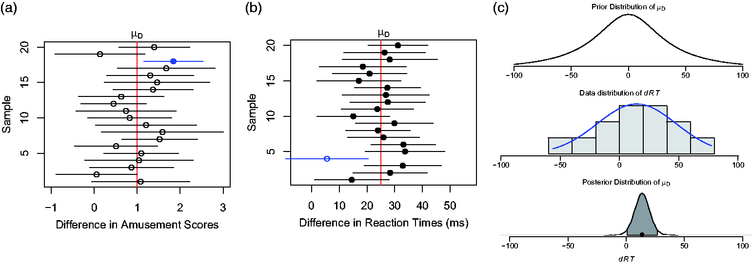
We conduct a t-test to evaluate the null hypothesis according to Fisher. The p-value is $P(T\ge \left|t\right||H_0)$ , where $t=\frac{{\overline{X}}_D-0}{s/\sqrt{N}}$ and T is the variable representing all possible values of t that might be obtained over repeated samples (the sampling distribution of t). Here, t(24) = 1.96, p = .0612, where $(N-1)=24$ are the degrees of freedom for the test statistic. The left plot of Figure 1 presents the sampling distribution of T. The observed statistic, $|t|$ is represented by the two vertical reference lines corresponding to $\pm 1.96$ , and the p-value of .0612 is represented by the sum of the two shaded areas more extreme than the observed t-test statistics. According to Fisher, when the p-value is small, the data are inconsistent with H₀. When the p-value is large, there is insufficient evidence against H₀, suggesting that more data should be obtained. Here, the p-value is relatively small suggesting that the data were less likely to have come from a population with ${\mu }_D=0$ .

Figure 1.

The left plot displays the sampling distribution of the t-test statistic for Sample 1. The blue line is the t-test value $t(24)=|1.96|$ and the shaded area represents the p-value $.0612$ . The middle plot displays frequentist 95% confidence intervals (CIs) of 20 samples of $N=25$ from a population with ${\mu }_D=1$ and $\sigma =2.5$ ; sample means are represented as circles and dots. The right plot shows the components to Bayesian inference. The prior distribution is ${\mu }_D\sim \sigma \mathit{Cauchy}(0,1)$ , with $\pi ({\sigma }^2)={\sigma }^{-2}$ (not shown). This histogram presents data from Sample 1 in the frequentist CI plot, with the fitted model overlaid as a normal curve. The shaded area in the posterior distribution for ${\mu }_D$ is the 95% Bayesian credible interval, and the dot represents the mean of the posterior.

If the null hypothesis was directional so that $H_0:{\mu }_D\le 0$ , it means that pouting elicits more amusement that smiling. The p-value associated with this directional hypothesis would be .0306 (the right tail probability of Figure 1). This p-value suggests that the data are less likely to have come from a family of populations with ${\mu }_D<0$ rather than from a population with ${\mu }_D=0$ . Considering different ways to specify H₀ is another aspect of statistical thinking.

With this information, a decision according to N-P theory can also be made by specifying some α or Type I error associated with testing $H_0:{\mu }_D=0$ before the data are analysed. Recall the context where a teacher will use this test to decide whether to implement this activity for the school year. When α = .05, he accepts $H_0:{\mu }_D=0$ because p = 0.0619 > .05, and does not implement pencil-holding-in-teeth in class. This decision is made independently of any alternative hypothesis H₁ in mind. Therefore, it does not imply that $H_1:{\mu }_D\ne 0$ is true. Note that this decision can be an error 5% of the time. Because the data was generated from a population with ${\mu }_D=1$ , the decision to accept $H_0:{\mu }_D=0$ is an error. If the teacher specifies α = .10 instead, he will reject H₀ and have the students hold pencils in their teeth.

Estimation

Recall that the estimation perspective focuses on effect sizes and their uncertainty or precision in estimation (e.g., Cumming, 2014). The estimated mean difference in amusement is ${\overline{X}}_D=1.1$ . On average, participants in the smile condition rated cartoons 1.1 more amusing than those in the pout condition.

The 95% CI equals $[-0.1,2.2]$ for the unknown mean difference ${\mu }_D$ . Over repeated samples of the population, 95% of intervals constructed identically to $[-0.1,2.2]$ contain the mean difference ${\mu }_D$ (known to be 1.0 in this case because we simulated the data). In the centre plot of Figure 1, 20 of such 95% CIs have been constructed for the facial feedback effect that was estimated by samples of $N=25$ . ⁹ Circles or a dot represent the estimated means, and lines intersecting the means represent the CIs. Five percent, or one out of 20, of these CIs (i.e., the dot representing sample 18) does not contain the unknown population mean difference, ${\mu }_D$ . The probability that any single CI contains ${\mu }_D$ is 0 or 1. The variability between means and their CIs from sample to sample in Figure 1 illustrates the random nature of data over the long run or frequentist sampling variability.

Relative to p-values, CIs shift focus away from hypotheses onto estimated effect sizes (e.g., ${\overline{X}}_D$ ) and communicate the extent of estimate precision by their widths: the smaller the CI, the more precise the estimate of the effect size. The frequentist results suggest that there is weak evidence in support of facial feedback: plausible estimates of ${\mu }_D$ (i.e., ${\overline{X}}_D$ ) tend to be positive but span a large range of values that can include 0.

Bayesian approach

Recall that the Bayesian perspective incorporates prior beliefs into the probability of an event. In lay terms, prior beliefs, represented by a probability distribution, are updated by data to obtain a posterior probability distribution. This posterior probability reflects the strength of belief that an event will occur from the perspective of the entity providing prior information (see Kruschke & Liddell, 2018 for an introduction).

Estimation

For the simulated example on the facial feedback effect, we assume that the likelihood of the data (difference scores) is normal with mean ${\mu }_D$ and variance ${\sigma }^2$ . Suppose we are sceptical and initially suspect that the facial feedback effect represented by ${\mu }_D$ is around 0. One useful Bayesian model that can be applied to experimental designs that are traditionally analysed with t-tests and analyses of variance uses a Jeffreys-Zellner-Siow (JZS) prior (see Ly, Verhagen, & Wagenmakers, 2016 for an introduction).

The right panel of Figure 1 shows this prior distribution for ${\mu }_D$ in the topmost plot. The histogram in the middle plot represents the simulated data; and the likelihood of the model fit to the data is represented as the superimposed normal distribution. Finally, the bottom plot presents the posterior distribution for ${\mu }_D$ , which is obtained from the multiplication of the prior (topmost plot) and the likelihood (middle plot).

The posterior distribution in the bottom plot in the right panel of Figure 1 represents our updated beliefs about ${\mu }_D$ after incorporating information from the data. The posterior distribution can be summarized by any reasonable statistic (e.g., the five number summary). The posterior mean or expectation of the posterior distribution $\mathbb{E}[{\mu }_D|x]$ and the posterior median are both 1.0, which is a reasonable effect size estimate. Beginning with the prior expectation of no facial feedback effect $\mathbb{E}[{\mu }_D|x]$ $({\mu }_D=0)$ , incorporating new data shifts the posterior expectation to a facial feedback effect of 1.0 points in difference amusement scores.

The posterior mean of 1.0 is a weighted average of the prior mean of 0 and the observed mean ${\overline{X}}_D=1.1$ . As the sample size becomes very large, $\mathbb{E}[{\mu }_D|x]$ and ${\overline{X}}_D$ approach the same value. The 95% Bayesian credible interval, BCI = [0.1, 3.3] maps onto the bounds of the shaded region of the posterior density in Figure 1. Given the observed data, there is 95% probability that the unknown ${\mu }_D$ falls within the interval [0.1, 3.3]. The BCI and posterior mean suggest a nonzero effect of facial feedback that can be close to 0.

Evaluation

Consider the Bayes factor ( ${\mathit{BF}}_{10}$ ), which, as described above quantifies the relative strength of evidence of H₁ against H₀. In this example, we use the same JZS prior as before and let $H_0:{\mu }_D=0.$ Additionally, we let $H_1:{\mu }_D\ne 0$ to take on any value except 0. Here, ${\mathit{BF}}_{10}=0.87$ , meaning that the evidence for H₁ is reduced to 87% of what it was before we observed the data.

We could formulate a competing alternative hypothesis distinct from $H_1:{\mu }_D\ne 0$ , which allows for negative values of ${\mu }_D$ . For example, we might want to evaluate the hypothesis $H_2:{\mu }_D>0$ using a BF. Then, ${\mathit{BF}}_{20}=1.7$ , suggesting that the evidence for H₂ is 1.7 times stronger than it was before observing the data. Additionally, we can compute ${\mathit{BF}}_{21}=1.9$ , indicating evidence in support of $H_2:{\mu }_D>0$ relative to $H_1:{\mu }_D\ne 0$ . Among the three competing hypotheses, H₂ is more likely, followed by H₀ and then H₁. With such close $\mathit{BF}$ values, the hypotheses are not strongly distinguishable from one another.

Summary

Statistical thinking requires the consideration of multiple sources of information. In this simulated example, the different approaches to statistical inference (see Table 1) obtain corroborating results consistent with a population mean of ${\mu }_D=1.$ Because statistics is about quantifying uncertainty, our sample mean is not exactly equal to the population mean as reflected in the 95% CI and BCI. Uncertainty is also reflected in the lack of strong distinctions among the hypotheses evaluated. Additionally, the decision rule we set up under N-P testing results in a decision error of behaving as though there was no facial feedback effect despite the effect being nonzero or true in the population.

The student should note that results from statistical procedures from a single dataset are not definitive because of uncertainty due to sampling variability. With one dataset, uncertainty regarding the (unknown) value of the population mean, ${\mu }_D$ , can be reduced when different statistical approaches applied to answering the same question have corroborative results. Consistent results obtained from different methods applied to the same data indicate a strong signal relative to noise in the data. Alternatively, to address uncertainty due to sampling variability, confidence is gained when hypothesized effects are repeatedly observed over a large set of replication studies. These points can be empirically demonstrated by drawing different samples from the same population in the simulation study and observing the variability in statistical results (e.g., see middle plot in Figure 1).

Empirical example: facial feedback

Unlike simulated data, psychological science investigates phenomena where the population parameters are unknown and data are examined for whether they support theories. Below, we demonstrate statistical thinking by applying the different statistical approaches to empirical data on the popular facial feedback hypothesis (Strack et al., 1988, which has almost 2000 citations according to Google scholar). This popularity provoked Wagenmakers et al. (2016) to publish a multi-lab registered replication report consisting of 17 replication studies. For our empirical example, we focus on analysing data from the 17th study by Zeelenberg, Zwaan, and Dijkstra (credited in Wagenmakers et al., 2016).

Zeelenberg et al. (credited in Wagenmakers et al., 2016) recruited 145 students to participate in the smile or pout condition, where they rated 4 cartoons on a 10-point scale ranging from 0 (I felt not at all amused) to 9 (I felt very much amused). The study protocol is documented on a video at https://osf.io/spf95/. Participants were excluded from analyses when their average cartoon ratings exceeded 2.5 standard deviations from the group mean in their condition (i.e., outliers), when they correctly guessed the goal of the study, when they indicated that they did not understand the cartoons, and when they did not hold the pen correctly with their mouth for two or more cartoons. The final sample consisted of N = 108 participants, with n = 50 in the smile condition and n = 58 in the pout condition.

Data analysis

Descriptive statistics

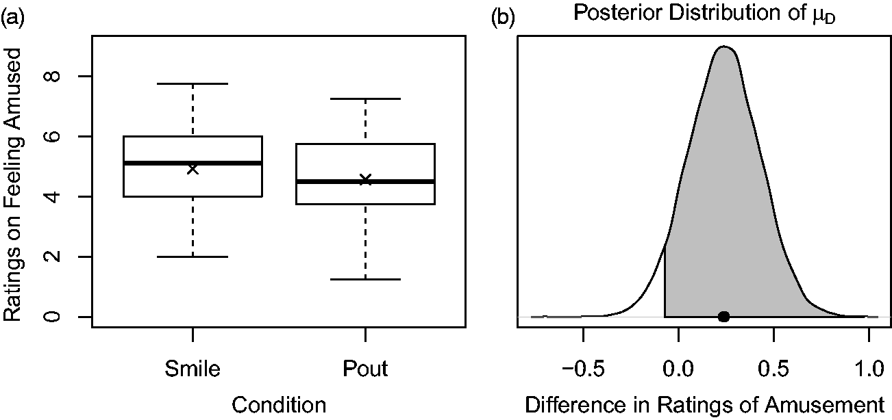
The left panel of Figure 2 presents boxplots of the amusement ratings by condition ( ${\overline{X}}_{\text{smile}}=4.93$ , $s_{\text{smile}}=1.40$ versus ${\overline{X}}_{\text{pout}}=4.58$ , $s_{\text{pout}}=1.41$ ). These means are consistent with the facial feedback hypothesis (i.e., ${\mu }_D>0$ , where ${\mu }_D={\mu }_{\text{smile}}-{\mu }_{\text{pout}}$ ). The means are represented by crosses, and the medians are represented by the bold vertical lines within the bars. The boxplots indicate no outliers (because they were removed according to the 2.5 standard deviation rule), suggest similar variances across the two conditions, and point to symmetry in the observed data distributions because the means are close to their medians. These preliminary analyses are important to ensure that downstream results are not invalidated by the presence of unusual cases or assumption violations (e.g., unequal variances).

Figure 2.

The left plot displays side-by-side box plots on ratings on feeling amused across four cartoons by the smile and pout conditions. Sample means per condition is represented by the crosses. The right plot is the posterior distribution $P({\mu }_D|x)$ . The shaded area represents the 90% probability that ${\mu }_D>0$ , and the dot represents the mean, $\mathbb{E}[{\mu }_D|x]=.24$ .

Frequentist statistics

The t-test of equal variances for $H_0:{\mu }_D\le 0$ gives the test statistic t(106) = 1.30, p = .0981. With a p-value that is not small, the value of ${\overline{X}}_D$ is consistent with random variability, diminishing the extent to which the alternative hypothesis ( $H_1:{\mu }_D>0$ ) provides a sensible explanation for the data. The facial posture manipulation resulted in a small difference score of ${\overline{X}}_D=0.35$ with 95% CI = [−0.2, 0.74]. Although the direction of the effect is positive, the scale of this effect lacks consequential meaning (cf. number of chuckles) for it to be informative. We do not apply the N-P approach here as the focus is on inferring the nature of an effect in the population and not behaviour.

Bayesian statistics

We used the JZS prior for these data, assuming equal variances, and obtained the posterior distribution of ${\mu }_D$ . Comparing $H_1:{\mu }_D>0$ against $H_2:{\mu }_D=0$ , we have ${\mathit{BF}}_{12}$  = 0.59. However, when we compare H₁ against $H_3:{\mu }_D<0$ , ${\mathit{BF}}_{13}$  = 8.6. Although the evidence supporting H₁ over H₃ is strong, H₂ is the most likely hypotheses ( ${\mathit{BF}}_{23}$ and ${\mathit{BF}}_{21}$ are both 1.7). Lacking a meaningful scale associated with the estimated effect, information about the effect size and its uncertainty is non-informative and not reported here. ¹⁰ To quantify the posterior probability of $H_1{\mu }_D>0$ , we observe that $P(H_1|x)=0.8978.$ This estimate of the posterior probability is interpreted as the probability that amusement scores are larger in the smile than pout condition is a close to 90% (see right panel of Figure 2). Code to reproduce these analyses is available at https://osf.io/5v8kw/.

Summary

Results from frequentist and Bayesian approaches do not always lead to the same conclusion. The frequentist results suggest that the data are noisy and one logical plan of action is to examine ways to reduce random error (e.g., develop a better measure of amusement) to obtain data inconsistent with $H_0:{\mu }_D\le 0$ . Although the posterior probability of $H_1:\mu >0$ that represents the facial feedback hypothesis is a large 90%, the $\mathit{BF}$ results suggest that relative to the three competing hypotheses, $H_2:{\mu }_D=0$ is most likely, followed by H₁, and then by $H_3:{\mu }_D<0$ as the most unlikely. Both approaches point to the need for less noisy data.

Discussion

Teaching statistics is challenging because of its abstraction, technicality, and complexity. We forward statistical thinking as a unifying learning objective that underlies four topics. First, we advocate distinguishing frequentist from Bayesian probability by appealing to intuition and illustrating concepts with simulation and graphics. Berry (1997) provides suggestions on how to introduce Bayesian concepts at the undergraduate level.

Second, students must be able to appreciate uncertainty in results. The role of statistics is to quantify uncertainty. How well students use information about uncertainty depends on their ability to think statistically. Students should recognize that the scientific endeavour is characterized by the motivation to reduce uncertainty while also appreciating that this uncertainty cannot be eliminated.

Third, students must recognize the importance of being a data detective. Empirical data often have unexpected characteristics that can only be discovered by exploration. Competing models or hypotheses must be developed with these unexpected characteristics in mind.

Fourth and finally, the use of statistical software and coding facilitates statistical thinking. As with any technical skill, consistent practice with incremental challenges is necessary to achieve coding mastery. Data Camp (https://www.datacamp.com/) provides free online courses to get started with R, and R code to accompany the two examples is provided in the supplementary material. We computed $\mathit{BF}$ s using the BayesFactor package in R (Morey, Rouder, & Jamil, 2015), and recommend the freely available JASP software (JASP Team, 2018) that can conduct both frequentist and Bayesian analysis. Compared with R, JASP has the advantage of a graphical user interface that minimizes the use of script-based programming.

Incorporating both Bayesian and frequentist approaches within a course is challenging, and we recommend teaching at least two different perspectives. With two approaches and sets of results, students are more likely to engage in statistical thinking instead of treating statistics akin to following a single “correct” recipe. The student who masters statistical thinking can flexibly approach research questions with a toolkit of related approaches, providing different insights to the data. Within this toolkit, students should recognize that statistical tests focus on one aspect of a model whereas scientific inquiry is moving toward the examination of models as a whole. Instead of seeking for answers with an eye for “fact finding,” students should approach research questions from different angles, considering alternative explanations of the data. Promoting statistical thinking is a first step towards thinking like a scientist and being savvy consumers of scientific results.