An In-Class Demonstration of Bayesian Inference

Abstract

Sir Ronald Fisher’s venerable experiment “The Lady Tasting Tea” is revisited from a Bayesian perspective. We demonstrate how a similar tasting experiment, conducted in a classroom setting, can familiarize students with several key concepts of Bayesian inference, such as the prior distribution, the posterior distribution, the Bayes factor, and sequential analysis.

Over 80 years ago, Sir Ronald Fisher conducted the famous experiment “The Lady Tasting Tea” in order to test whether his colleague, Dr Muriel Bristol, could taste if the tea infusion or the milk had been added to the cup first (Fisher, 1937, p. 11). Dr Bristol was presented with eight cups of tea and the knowledge that four of these had the milk poured in first. Dr Bristol was then asked to identify these four cups. Fisher analyzed the results using null hypothesis significance testing:

1. Assume the null hypothesis to be true (i.e., Dr Bristol lacks any ability to discriminate the cups).

2. Calculate the probability of encountering results at least as extreme as those observed.

3. If that probability is sufficiently low, consider the null hypothesis discredited.

This probability is now known as the p-value and it features in many statistical analyses across empirical sciences such as biology, economics, and psychology (for recent critique, see Benjamin et al., 2018; Wasserstein & Lazar, 2016).

Decades later, Dennis Lindley (1993) used an experimental procedure similar to that of Fisher to highlight some limitations of the p-value paradigm. Specifically, the calculation of the p-value depends on the sampling plan, that is, the intention with which the data were collected. Consider the Lindley setup: the lady is offered six pairs of cups, where each pair consists of a cup where the tea was poured first, and a cup where the milk was poured first. She is then asked to judge, for each pair, which cup has had the tea added first. A possible outcome is the sequence RRRRRW, indicating that she was right for the first five pairs, and wrong for the last pair. However, as Lindley demonstrated, the original sampling plan is crucial in calculating the p-value. Was the goal to have the lady taste six pairs of cups – no more, no less – or did she need to continue until she made her first mistake? The observed data are compatible with either sampling plan; yet in the former case, the p-value equals 0.109, whereas in the latter case the p-value equals 0.031. The difference lies in the inclusion of more extreme cases. In the “test six cups” plan, the only more extreme outcome is RRRRRR (i.e., the binomial sampling distribution), whereas for the “test until error” plan the more extreme outcomes include sequences such as RRRRRRW and RRRRRRRW (i.e., the negative binomial sampling distribution). It seems undesirable that the p-value depends on hypothetical outcomes that are in turn determined by the sampling plan. Harold Jeffreys summarized: “What the use of p implies, therefore, is that a hypothesis that may be true may be rejected because it has not predicted observable results that have not occurred. This seems a remarkable procedure” (Jeffreys, 1961, p. 385; see also Berger & Wolpert, 1988).

In this article we revisit Fisher’s experimental paradigm to demonstrate several key concepts of Bayesian inference, specifically the prior distribution, the posterior distribution, the Bayes factor, and sequential analysis. Furthermore, we highlight the advantages of Bayesian inference, such as its straightforward interpretation, the ability to monitor the result in real-time, and the irrelevance of the sampling plan. For concreteness, we analyze the outcome of a tasting experiment that featured 57 staff members and students of the Psychology Department at the University of Amsterdam; these participants were asked to distinguish between the alcoholic and the non-alcoholic version of the Weihenstephaner Hefeweissbier, a German wheat beer. We describe how classroom tasting experiments can acquaint students with Bayesian inference, noting that beer can be substituted with anything else suitable (e.g., red and green M&M’s, Coca Cola and Pepsi, decaf and regular coffee). We analyze and present the results in the open-source statistical software JASP (JASP Team, 2019).

The Tasting Experiment

On a Friday afternoon, May 12th 2017, an informal beer tasting experiment took place at the Psychology Department of the University of Amsterdam. The experimental team consisted of three members: one to introduce the participants to the experiment and administer the test, one to pour the drinks, and one to process the data. Participants tasted two small cups filled with Weihenstephaner Hefeweissbier, one with alcohol and one without, and indicated which one contained alcohol. Participants were also asked to rate the confidence in their answer (measured on a scale from 1 to 100, with 1 being completely clueless and 100 being absolutely sure), and to rate the two beers in tastiness (measured on a scale from 1 to 100, with 1 being the worst beer ever and 100 being the best beer ever). The experiment was double-blind, such that the person administering the test and interacting with the participants did not know which of the two cups contained alcohol. For ease of reference, each cup was labeled with a random integer between 1 and 500, and each integer corresponded either to the alcoholic or non-alcoholic beer. A coin was flipped to decide which beer was tasted first. The setup was piloted with nine participants; subsequently, we tested as many people as possible within an hour, and also recorded which of the two beers was tasted first. On average, testing took approximately 30 seconds per participant, yielding a total of 57 participants. Of the 57 participants, 42 (73.7%) correctly identified the beer that contained alcohol; in other words, there were s = 42 successes and f = 15 failures. ¹

Theoretical Analysis

In order to assess statistically whether and to what extent participants were able to discriminate between alcoholic and non-alcoholic beer we apply the binomial model, where the rate parameter θ governs the probability of a correct response for each of the participants. Chance performance corresponds to $\theta =1/2$ . Above-chance performance corresponds to values of θ higher than $1/2$ , with θ = 1 indicating perfect performance.

In the Bayesian framework, we start by specifying a prior distribution. The prior distribution quantifies our beliefs about the parameter of interest before seeing the data. For convenience, we may specify a beta distribution: a probability distribution on the domain $[0,1]$ governed by two shape parameters, a and b. Setting $a=b=1$ yields a uniform distribution, and implies that all values of rate θ are equally likely a priori. Setting a > b assigns more prior probability mass to values of θ higher than $1/2$ , whereas setting a < b assigns more mass to values of θ lower than $1/2$ . ²

The beta prior distribution is then updated to a posterior distribution using Bayes’ rule, such that values of θ that predicted the data well receive a boost in credibility, whereas values of θ that predicted the data poorly suffer a decline (Rouder & Morey 2017; Wagenmakers et al., 2016):

$$\underset{\text{Posterior}}{\underbrace{p(\theta |s,f)}}=\underset{\text{Prior}}{\underbrace{p(\theta )}}\times \stackrel{\text{Predictionforspecific}\theta }{\overbrace{\underset{\genfrac{}{}{0ex}{}{\text{Averageprediction}}{\text{acrossall}\theta \text{'}\text{s}}}{\underbrace{\frac{p(s,f|\theta )}{p(s,f)}}}}}$$

(1)

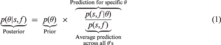
The right-most term is the predictive updating factor that quantifies the change from prior to posterior beliefs brought about by the data. This predictive updating factor indicates how well each value of θ predicted the data, relative to the average prediction across all values of θ. When a specific value of θ predicted the data better than average, the posterior density at that point will be higher than the prior density.

We used the binomial likelihood to assess the quality of each value’s prediction (i.e., the likelihood of observing s successes and f failures, given a specific value of θ). Because we used the binomial likelihood and a beta prior distribution, the updated posterior distribution will also be a beta distribution – a property known as conjugacy (Gelman et al., 2003).

The obtained posterior distribution can be used for both parameter estimation and hypothesis testing. For parameter estimation, either a point estimate or an interval estimate can be obtained. Commonly used point estimates include the posterior median and posterior mean. Interval estimation can be done with a so-called credible interval, which is an interval that contains x% of the posterior mass ³ and can be interpreted as follows: there is an x% probability that the true parameter lies in this interval. For example, if we obtain a 95% credible interval of $[0.6,0.9]$ for θ, we can be 95% sure that the true value of θ lies between 0.6 and 0.9.

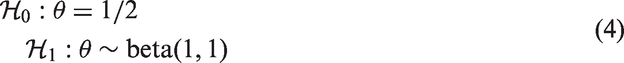
The posterior distribution can also be used for hypothesis testing, where the traditional goal is to examine specific values of θ. For instance, we can test the hypothesis ${\mathcal{H}}_0⋮\theta =1/2$ (i.e., chance performance) by comparing its predictive adequacy to that of an alternative hypothesis ${\mathcal{H}}_1⋮\theta \ne 1/2$ . In other words, ${\mathcal{H}}_0$ represents the idealized position of a skeptic who believes that the data can be accounted for purely by chance. This “chance only” model is pitted against an alternative that allows θ to take on values different from $1/2$ .

As before, hypotheses that predict the data well receive a boost in credibility, whereas hypotheses that predict the data poorly suffer a decline. In the Bayesian framework, hypothesis testing is traditionally achieved through the Bayes factor (Etz & Wagenmakers, 2017; Kass & Raftery, 1995). ⁴ The Bayes factor can be seen as a weighing of one hypothesis’ predictive quality relative to that of another. The following equation illustrates this principle, and is very similar to equation (1):

$$\underset{\genfrac{}{}{0ex}{}{\text{Posteriorbeliefs}}{\text{abouthypotheses}}}{\underbrace{\frac{p({\mathcal{H}}_1|s,f)}{p({\mathcal{H}}_0|s,f)}}}=\underset{\genfrac{}{}{0ex}{}{\text{Priorbeliefs}}{\text{abouthypotheses}}}{\underbrace{\frac{p({\mathcal{H}}_1)}{p({\mathcal{H}}_0)}}}\times \underset{\text{Bayesfactor}}{\underbrace{\frac{p(s,f|{\mathcal{H}}_1)}{p(s,f|{\mathcal{H}}_0)}}}$$

(2)

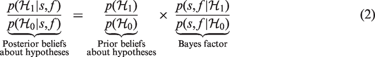
It is important to note here that the Bayes factor is a relative metric of the hypotheses’ predictive quality. For instance, if the Bayes factor equals 5, this means that the data are 5 times as likely under ${\mathcal{H}}_1$ than under ${\mathcal{H}}_0$ . The relative nature of the Bayes factor stands in stark contrast with the frequentist paradigm, where only the null hypothesis is under consideration.

The computation of the Bayes factor is usually not straightforward; however, when the two hypotheses are nested, a convenient computational shortcut can be used, known as the Savage–Dickey density ratio (Dickey & Lientz, 1970; Wagenmakers et al., 2010). The shortcut entails that the Bayes factor equals the ratio of the prior density and the posterior density at the test value θ₀. For instance, in the current study, ${\theta }_0=1/2$ so we have the following ratio:

$${\text{BF}}_{10}=\frac{p(\theta =1/2)}{p(\theta =1/2|\text{data})}$$

(3) where the numerator indicates the prior ordinate and the denominator indicates the posterior ordinate evaluated at the test value, $\theta =1/2$ . BF denotes the Bayes factor, and the subscript indicates which hypotheses are compared. ${\text{BF}}_{10}$ indicates the Bayes factor in favor of ${\mathcal{H}}_1$ $(\text{i}.\text{e}.,\frac{\text{p}(\text{data}|{\mathcal{H}}_1)}{\text{p}(\text{data}|{\mathcal{H}}_0)})$ , whereas ${\text{BF}}_{01}$ indicates the Bayes factor in favor of ${\mathcal{H}}_0$ $(\text{i}.\text{e}.,\frac{\text{p}(\text{data}|{\mathcal{H}}_0)}{\text{p}(\text{data}|{\mathcal{H}}_1)})$ . For instance, if ${\text{BF}}_{10}=1/5$ , then ${\text{BF}}_{01}=5$ .

We stress that the mathematical details are not critical for students’ understanding of the Bayesian procedures. The following section shows how the example and the associated graphs suffice to clarify the key Bayesian concepts at an intuitive level.

Bayesian Inference with JASP

When the statistical explanation does not resonate with students, a practical demonstration of the analysis might. This can be done with the statistical software JASP, which offers a graphical user interface for conducting Bayesian (and frequentist) analyses. In order to analyze the collected data, the Bayesian binomial test can be used, which can be found under the menu labeled “Frequencies”. Several settings are available for the binomial test, allowing students to explore different analysis choices. Figure 1 presents a screenshot of the options panel in JASP. For this analysis, we specify a test value of $1/2$ (i.e., chance performance), and $a=b=1$ for the prior distribution of θ under ${\mathcal{H}}_1$ . Note that in a sensitivity or robustness analysis, other values for a and b may be explored to assess their impact on the posterior distribution.

Figure 1.

The input panel for the Bayesian binomial test in JASP. The upper-left box displays all available variables. The upper-right box displays the tested variables. Below are other options, such as setting the test value, the alternative hypothesis, and the shape parameters of the beta prior.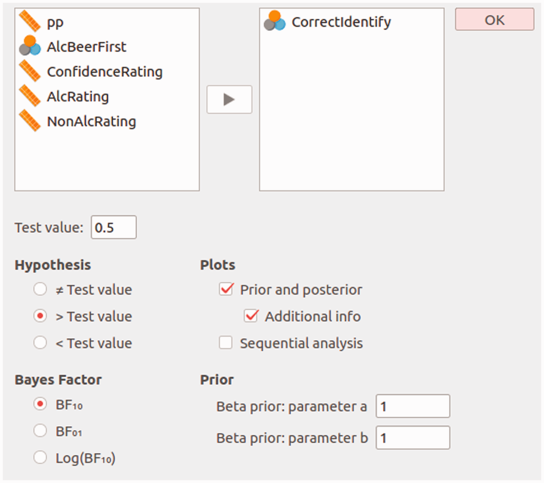

The null hypothesis postulates that participants performed at chance level, whereas the alternative hypothesis postulates that this is not the case. For instance, in the case of two-sided hypothesis testing, the hypotheses are specified as follows

$$\begin{array}{c}{\mathcal{H}}_0⋮\theta =1/2\\ {\mathcal{H}}_1⋮\theta \sim \text{beta}(1,1)\end{array}$$

(4)

However, since we wish to test whether or not participants’ discriminating ability exceeds chance, we can specify the alternative hypothesis to allow only values of θ greater than $1/2$ (note the ‘+’ in the subscript):

$${\mathcal{H}}_{+}⋮\theta \sim \text{beta}(1,1)\text{I}(1/2,1)$$

(5) where I indicates truncation of the beta distribution to the interval $[1/2,1]$ .

Figure 2 illustrates the results of the binomial test. The left panel shows the prior and the posterior distribution of θ for the two-sided alternative hypothesis, along with the median and credible interval of the posterior distribution. The posterior median equals 0.731 and the 95% credible interval ranges from 0.610 to 0.833, indicating a substantial deviation of θ from $1/2$ . For each value of θ, the change from prior distribution to posterior distribution is quantified by predictive adequacy: for those values of θ that predict the data better than average, the posterior density exceeds the prior density (see equation (1)). The left panel shows inference for the two-sided alternative hypothesis (i.e., ${\mathcal{H}}_1⋮\theta \ne 1/2$ ) compared to the null hypothesis (i.e., ${\mathcal{H}}_0⋮\theta =1/2$ ). The resulting Bayes factor is 122.65 in favor of the alternative hypothesis, that is, the observed data are about 123 times more likely to occur under ${\mathcal{H}}_1$ than under ${\mathcal{H}}_0$ .

Figure 2.

Bayesian binomial test for the rate parameter θ. The probability wheel at the top illustrates the ratio of the evidence in favor of the two hypotheses. The two gray dots indicate the prior and posterior density at the test value—the ratio of these is the Savage–Dickey density ratio. The median and the 95% credible interval of the posterior distribution are shown in the top-right corner. The left panel shows the two-sided test and the right panel shows the one-sided test. Both figures from JASP. (a) 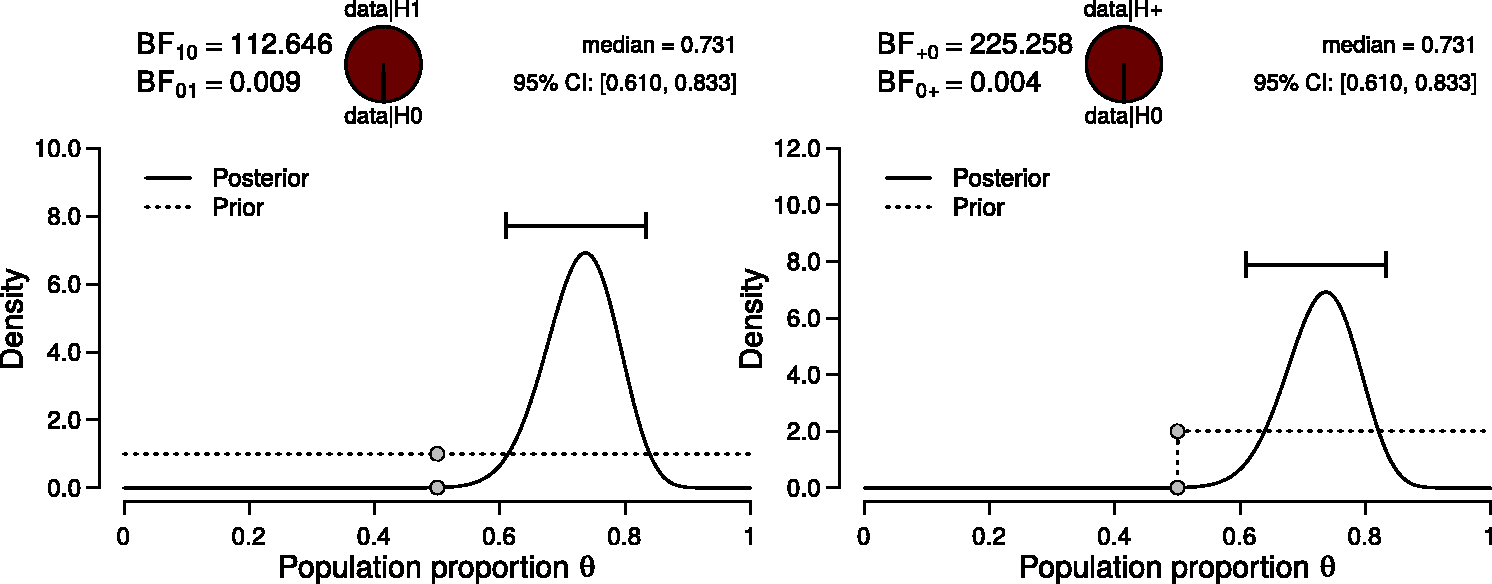${\mathcal{H}}_0⋮\sim \mathit{beta}(1,1)$ and (b) ${\mathcal{H}}_0⋮\sim \mathit{beta}(1,1)I(1/2,1)$ .

The right panel shows inference for the one-sided positive hypothesis (i.e., ${\mathcal{H}}_{+}⋮\theta \ge 1/2$ ) compared to the null hypothesis: the resulting Bayes factor is 225.26 in favor of the alternative hypothesis. Note that the posterior distribution itself has hardly changed: the posterior median still equals 0.731 and the 95% credible interval ranges from 0.610 to 0.833. Because virtually all posterior mass was already to the right of $1/2$ in the two-sided case, the posterior distribution was virtually unaffected by changing from ${\mathcal{H}}_1$ to ${\mathcal{H}}_{+}$ . However, in the right panel, ${\mathcal{H}}_{+}$ only predicts values greater than $1/2$ , which is reflected in the prior distribution: all prior mass is now located in the interval $(1/2,1)$ , and as a result, the prior mass in the interval $(1/2,1)$ has doubled. Since the posterior density at the point of testing is the same in both panels, but the prior density is doubled in the right panel, the Bayes factor for the directed hypothesis doubles as well.

The experimental procedure also highlights one of the main strengths of Bayesian inference: real-time monitoring of the incoming data. As the data accumulate, the analysis can be continuously updated to include the latest results. In other words, the results may be updated after every participant, or analyzed all at once, without affecting the resulting inference. To illustrate this, we can use Equation 1 to compute the posterior distribution for the first nine participants of the experiment for which s = 6 and f = 3. Specifying the same beta prior distribution as before, namely a truncated beta distribution with shape parameters $a=b=1$ , and combining this with the data, yields a truncated beta posterior distribution with shape parameters $a=6+1=7$ and $b=3+1=4$ . ⁵ The resulting posterior distribution is presented in the left panel of Figure 3. Now, we can take the remaining 48 participants and conduct the Bayesian binomial test. Because we already have knowledge about the population’s rate parameter θ, namely the results of the first nine participants, we can incorporate this in the analysis through the prior distribution, following Lindley’s maxim “today’s posterior is tomorrow’s prior” (Lindley, 1972).

Figure 3.

Sequential updating of the Bayesian binomial test. The left panel shows results from a one-sided Bayesian binomial test for the first n = 9 participants (s = 6, f = 3). The shape parameters of the truncated beta prior were set to a = 1 and b = 1. The right panel shows results from a one-sided binomial test for the remaining 48 participants. Here, the specified prior is the posterior distribution from the left panel: a truncated beta distribution with 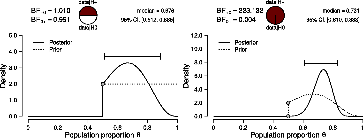$a+s=7$ and $b+f=4$ . The resulting posterior distribution is identical to the posterior distribution in Figure 2(b). In order to obtain the total Bayes factor in Figure 2(b), the component Bayes factors in Figures 3(a) and 3(b) can be multiplied (Jeffreys, 1937). Both figures from JASP. (a) n = 9 and (b) n = 57.

In this case, we can specify a truncated beta prior distribution with a = 7 and b = 4, and update this with the data of the remaining 48 participants using Equation 1. Out of the 48 participants, 36 were correct, and 12 were incorrect. Updating the prior distribution with this data yields a posterior distribution with shape parameters $a=7+36=43$ and $b=4+12=16$ , which is exactly the same posterior distribution obtained when analyzing the full data set at once. This two-step procedure is illustrated in Figure 3. The left panel shows the prior distribution (i.e., the truncated beta distribution with $a=1,b=1$ ) and the posterior distribution for the first nine participants. The right panel shows the inference for the remaining 48 participants, while incorporating the knowledge gained from the first nine participants in the prior distribution by specifying a truncated beta distribution with $a=7,b=4$ .

The ability to monitor the data in real-time and update the inference accordingly prevents wasteful data collection: if there is sufficient evidence to discredit either hypothesis with 50 observations, why collect another 10? Wasteful testing is a serious issue, and monitoring the evidence is important in fields such as medicine, biology, and industry. The Bayesian framework for planning experiments is discussed in more detail by Rouder (2014), Schönbrodt & Wagenmakers (2018), and Schönbrodt et al. (2017). Figure 4 shows the evolution of the Bayes factor as more data are collected. Initially the evidence is inconclusive, but after 30 participants the evidence increasingly supports ${\mathcal{H}}_1$ .

Figure 4.

Sequential analysis, showing the evolution of the Bayes factor as n, the number of observed participants, increases. After an initial period of inconclusiveness, the Bayes factor strongly favors 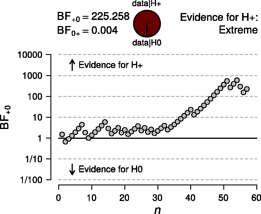${\mathcal{H}}_1$ . Figure from JASP.

Concluding Remarks

This article has outlined a teaching tool for familiarizing students with the basics of Bayesian inference. The educational advantage of the Bayesian binomial test is that both the likelihood function and the parameterization of the prior and posterior distributions are intuitive and straightforward. The tasting experiment allows students to analyze their own data, collected on the fly, making the inferential process more concrete and relevant. Table 1 summarizes the concepts that are introduced during the tasting experiment, as well as how these concepts can be practically demonstrated. The experiment is aimed at introducing college-level students to these concepts. We have positive experiences using it as a teaching tool in both introductory workshops and undergraduate courses in Bayesian inference.

Table 1.

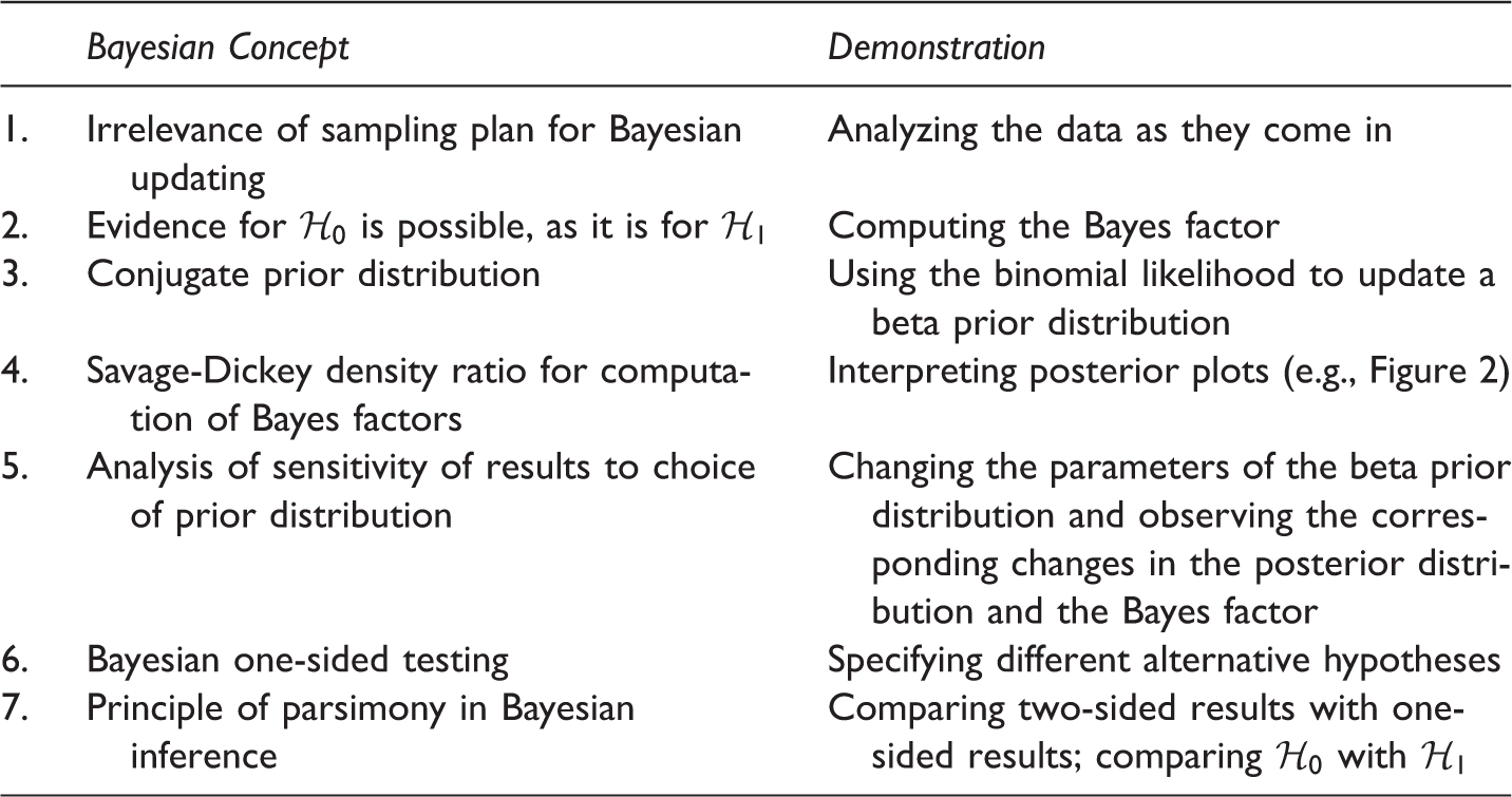
Bayesian concepts that students will learn during the tasting experiment and how these concepts can be demonstrated

	Bayesian Concept	Demonstration
1.	Irrelevance of sampling plan for Bayesian updating	Analyzing the data as they come in
2.	Evidence for ${\mathcal{H}}_0$ is possible, as it is for ${\mathcal{H}}_1$	Computing the Bayes factor
3.	Conjugate prior distribution	Using the binomial likelihood to update a beta prior distribution
4.	Savage-Dickey density ratio for computation of Bayes factors	Interpreting posterior plots (e.g., Figure 2)
5.	Analysis of sensitivity of results to choice of prior distribution	Changing the parameters of the beta prior distribution and observing the corresponding changes in the posterior distribution and the Bayes factor
6.	Bayesian one-sided testing	Specifying different alternative hypotheses
7.	Principle of parsimony in Bayesian inference	Comparing two-sided results with one-sided results; comparing ${\mathcal{H}}_0$ with ${\mathcal{H}}_1$

We have created an Open Science Framework repository that contains the original data set, as well as a fully annotated JASP-file that presents additional analyses, such as a t-test on the difference in ratings for the alcoholic and non-alcoholic beer. The repository can be found at http://tinyurl.com/yyyc928g.

Declaration of Conflicting Interests

The author(s) declared no potential conflicts of interest with respect to the research, authorship, and/or publication of this article.

Funding

The author(s) disclosed receipt of the following financial support for the research, authorship, and/or publication of this article: This work was supported in part by a Vici grant from the Netherlands Organization of Scientific Research awarded to EJW (016.Vici.170.083). DM is supported by a Veni grant (451-15-010) from the Netherlands Organization of Scientific Research (NWO).