Numerical and experimental investigation of aerodynamic noise from a cooling fan in a turbulent flow

Abstract

The investigation into aerodynamic noise arising from rotating surfaces bears significant practical implications. Among these, engine cooling fans have persistently been identified as primary contributors to vehicle noise. This study aims to provide a deeper comprehension of the complex unsteady flow dynamics surrounding an automotive cooling fan and its consequential impact on the generation of aerodynamic noise. Prediction of sound generated from fluid flow, despite its difficulty, can be simulated using modern numerical techniques and computational fluid dynamics (CFD). This research undertakes both numerical and experimental investigations. The experiment involves evaluating fan pressure against mass flow rate at 1500 rpm, while aerodynamic noise assessment transpires at two rotational speeds of 1500 rpm and 2500 rpm. Empirical sound pressure level data of the fan is meticulously captured using the requisite measurement apparatus. In addition, numerical investigations of the aerodynamic noise of an automotive cooling fan based on computational fluid dynamics and computational aeroacoustic (CAA) method have been performed. Initially, a steady-state aerodynamic simulation is carried out, followed by the simulation of the flow field through the application of the improved delayed detached eddy simulation (IDDES) formulation. The pressure rise of the fan versus the mass flow rate is obtained. The satisfactory concurrence observed between the simulation outcomes derived from the numerical method and the experimental dataset stands as notable validation. For the aeroacoustic computation, the Ffowcs Williams-Hawkings model is invoked to deduce sound pressure levels at specific flow points. The broadband noise sources model is also used to obtain the sound power level on the blade surface. Conclusively, it emerges that maximal noise manifestation occurs at a 90° degree angle, corresponding to the hub’s frontal orientation, with discernible dominance of tonal noise within lower frequency ranges (sub-1000 Hz).

Introduction

Noise is a modern social problem that has been considered in various fields in recent years due to the progress of societies. For example, in recent years, noise reduction requirement has increased with the increasing number of automobiles. In Internal Combustion Engine (ICE) vehicles, the primary sources of noise are typically engine and road noise, particularly at lower speeds. However, it is noteworthy that in specific driving conditions, such as urban settings and traffic scenarios, the cooling fan has been recognized as a significant contributor to vehicle noise, distinct from engine noise.^1,2 This acknowledgment underscores the importance of considering the cooling fan as a notable noise source, particularly in certain operational contexts. It should be noted that the cooling fan is an essential component of vehicles that use a combustion engine. Thus, it is necessary to reduce automotive cooling fan noise. ³ Cooling fan module noise comprises aerodynamic noise, vibration/mechanical noise, and electromagnetic noise, with aerodynamic noise being the predominant factor. The subject of aerodynamically generated noise became of considerable interest around 1950 as a result of the appearance of the aircraft jet engine. The basic sound sources are monopole, dipole, and quadrupole. The physical significance of the basic sound sources, namely, the monopole, dipole, and quadrupoles are described in relation to their occurrence in compressors and fans, and to their consequent radiation characteristics by Powell. ⁴

In recent years, academia and industry have made efforts to propose noise reduction solutions. Pignier ⁵ stated that the development of more silent vehicles now requires the repetition of design through prototyping and wind tunnel testing. However, as these methods are costly and time-consuming, more manufacturers are relying on numerical methods.

One of the most important applications that has been considered in the field of noise reduction is aeroacoustic. The aeroacoustic analysis is commonly used to identify noise sources and in redesigning the equipment identified as the source of sound. In most numerical studies, aeroacoustic modeling is based on the FW–H equation and it considers the mean velocities obtained from the CFD analysis to estimate overall sound pressure level (OSPL) values. The FW–H equation considers only the surface monopole and dipole noise sources and it is an exact rearrangement of the continuity and the momentum in the form of an inhomogeneous wave equation. These methods are widely used to predict jet and rotor noise, see for instance West and Caraeni ⁶ and Suresh et al. ⁷ The FW–H equation, derived from the most common form of the Lighthill acoustic analogy, is able to calculate the sound produced by multiple acoustic sources. For example, Krishna et al. ⁸ reduced the motor fan noise using CFD and CAA simulations.

The study of axial flow machines from an acoustical viewpoint can be said to have begun with Gutin ⁹ ; whose work on propeller noise was the basis of most of the advances made during the next 20 years. Since then, Lighthill’s development of aerodynamic sound theory, ¹⁰ and in particular Curle’s extension of the theory in 1955 to include solid boundaries, ¹¹ have been recognized as a general foundation for further work in this area. The study of noise generation mechanisms in axial fans started with Sharland. ¹² They presented the various possible mechanisms of noise generation in axial flow fans. Neise ¹³ presented a review of axial flow fan noise generation mechanisms and control methods that deal with noise sources and generation mechanisms in axial flow fans. With the emergence of high-speed digital computers, the utilization of numerical simulations to predict noise gained significant advantages in identifying noise sources and elucidating generation mechanisms within turbomachines, particularly axial fans. ⁸

For instance, Maaloum et al. ¹⁴ made an aeroacoustic performance evaluation of axial flow fans based on the unsteady pressure field on the blade surface. Suzuki and Soya ¹⁵ studied the noise reduction for automotive radiator cooling fans. Amoiridis et al. ¹ predicted axial flow fan broad-band noise using LES. Nashimoto et al. ¹⁶ detected the aerodynamic noise sources over a rotating radiator fan blade for automobiles. Udawant et al. ¹⁷ predicted fan noise using CFD and made its validation. Lee and Nam ¹⁸ developed a low-noise cooling fan using uneven fan blade spacing.

Yoshida et al.3 studied the reduction of the blade passing frequency (BPF) noise radiated from an engine cooling fan. The purpose of this work was to find sound sources of the BPF noise by measuring sound intensity and analyzing the flow structure around the blade by CFD. Khelladi et al. ¹⁹ predicted tonal noise from a high rotational speed centrifugal fan. Udawant et al. ²⁰ designed and developed a radiator fan for automotive applications. Tannoury et al. ²¹ studied the influence of blade compactness and segmentation strategy on tonal noise prediction of an automotive engine cooling fan. Gérard et al. ²² made the use of a beat effect for the automatic positioning of flow obstruction to control tonal fan noise by theory and experiments. Ota et al. ²³ developed a highly efficient radiator cooling fan for automotive applications. Becher and Becker ²⁴ investigated the applicability of numerical noise prediction of an axial vehicle cooling fan. Zanon et al. ²⁵ made a numerical investigation of the location and coherence of broadband noise sources for a low-speed axial fan. The aerodynamic noise characteristics of an axial cooling fan were studied by Mo and Choi. ²⁶ They studied the analysis of the noise sources generated by the fan using an LES and FW-H method through the commercial CFD software.

In the present study, numerical simulations are carried out using a hybrid method of the improved delayed detached eddy simulation (IDDES) ²⁷ and the FW-H equation. ²⁸ The flow simulation employs the IDDES approach, while noise prediction is conducted through the utilization of the FW-H method. In some of the previous studies, Ottersten et al. ²⁹ and Sanjose and Moreau ³⁰ ; the unsteady Reynolds-averaged Navier Stokes (URANS) equations were adopted for the flow simulation. Additionally, it was found in a recent study by Ottersten et al. ³¹ that the aerodynamic forces obtained using the URANS are in good agreement with experimental data. Although this method is well coupled with the acoustic analogy and predicts the principal tonal noise well but not the broadband noise. The reason is that the URANS cannot resolve transient small-scale flow fluctuations that are also noise sources, although large-scale unsteady contents are captured. The IDDES, by contrast, simulates most of the fluctuations despite the modeling of sub-grid scale quantities. Hence, coupling the IDDES with the FW-H equation enables accurate prediction for both tonal and broadband noise, as was reported in previous studies on vehicle cooling fans by Rynell et al. ³² and Rynell et al. ³³ However, there are few studies that performed such a practice accurately. In the present study, the car cooling fan module is considered and its aerodynamic noise is investigated. In this research, acoustic simulation of a car radiator fan is performed using the finite volume method, obtained from STAR-CCM+ ³⁴ software. An experimental test was done to validate the aerodynamic results. Also, to measure the noise, an experimental test of two rotational speeds was performed. Interesting results concerning the SPL at different distances from the fan are obtained. Including the fact that tonal sound is the main component of aerodynamic sound. Moreover, It is observed that the sound field has a strong axial dipole characteristic at low frequencies while axial deviation occurs at high frequencies.

The chosen rotational speeds, 1500 rpm and 2500 rpm, correspond to low and high operational conditions of the car fan, respectively. These speeds were selected to capture the fan’s performance across a range of practical scenarios. The angles of 0° and 90° were chosen based on the position of cars in traffic and their relevance to urban noise pollution. In this context, 90° represents the forward position upstream of the fan, considering the expected symmetric sound radiation commonly observed in such configurations. ¹

The selected fan geometry is specifically tailored to an automotive model that plays a substantial role in contributing to noise pollution within the persistent traffic conditions experienced on highways and roads. In the present study, we bring novelty through an exploration of this particular fan geometry, representing the first comprehensive investigation of its noise characteristics. Our dual approach, combining numerical and experimental methods, strengthens the depth of our findings. Simultaneously, we examine the effects of angle, distance, and rotational speed on fan noise, contributing fresh insights to the field.

The rest of this paper is organized as follows. The next session explains the numerical method and the turbulence modeling approaches used. Then, the details of the geometry of the problem are introduced. The following section explains the equipment for the experimental measurements. After that results are discussed. Finally, the main conclusions of the work are presented in the last section.

Numerical methods and turbulence modeling

Aerodynamics

The flow simulations are performed utilizing the commercial software STAR-CCM+ ³¹ double precision. As the noise generated by a fan running at subsonic speed is primarily attributed to the fluctuating surface pressure exerted on the surrounding fluid, ³⁵ the aerodynamic calculations are performed assuming that density is constant. Governing equations characterizing the unsteady flow are the incompressible versions of continuity and Navier–Stokes equations, that is

$\frac{\partial {\overline{u}}_i}{\partial x_i}=0$

(1)

$\frac{\partial {\overline{u}}_i}{\partial t}+{\overline{u}}_j\frac{\partial {\overline{u}}_i}{\partial x_j}=-\frac{1}{\rho }\frac{\partial \overline{p}}{\partial x_i}+\frac{\partial }{\partial x_j}\left(\nu \frac{\partial {\overline{u}}_i}{\partial x_j}\right)-\frac{\partial {\tau }_{i,j}}{\partial x_j}$

(2)

In equation (2), u _j is the velocity in direction j, ρ is the density, p is the pressure and τ_i,j denotes the Reynolds stress tensor. The meaning of the overbar (−) on the flow variables depends on the turbulence methodology applied. In URANS mode, it corresponds to a time-averaged quantity whereas in LES mode, it represents a filtered quantity. As such, the unresolved momentum fluxes denoted by τ_i,j for the former technique represent all turbulence except for certain low-frequency modes in time. However for LES, the term accounts for the contribution from turbulent scales smaller than the computational grid. In either case, the term is unknown and is modeled by the Boussinesq assumption with an appropriate definition of turbulent viscosity.

Improved delayed detached eddy simulation

To correctly simulate high Reynolds number flows that contain a large range of turbulent scales, scale-resolving techniques are needed to capture the key features that govern noise production from subsonic fans. Hence, although LES alleviates uncertainties related to turbulence modeling, it imposes a severely increased computational cost compared to URANS. The main strategy to reduce the computational cost associated with wall-resolved LES, is by allowing hybridization of the LES technique with URANS, where boundary layers are simulated by the URANS and LES is employed in the remaining volume. This lays the foundation for the numerical strategy known as detached eddy simulation (DES). ³⁶ A number of shortcomings were addressed at the time of publication. Some were detected later on and were dealt with by the extended DES version which is the delayed detached eddy simulation (DDES). ³⁷ Although the DES methodology was primarily intended to use the URANS modeling in the entire attached boundary layer, recent versions allow LES to act within the boundary layer region. As such, wall-modeled LES (WMLES) capability represents a useful extension of the DES methodology. This motivated Shur et al. ²⁷ to formulate IDDES by blending the functionalities of DDES and WMLES. Depending on the inflow of turbulent content, IDDES responds differently: treating the boundary layer flows in either DDES ³⁷ or WMLES ³⁸ mode, respectively. An essential feature of IDDES is the new definition of the grid filter which depends on both the grid spacing and the wall distance. The formula for the grid filter is

$△=\mathit{min}\left(\mathit{max}\left[0.15d_W,0.15h_{\mathit{max}},h_{wn}\right],h_{\mathit{max}}\right),$

(3)

Where d _W is the distance to the wall, h _max is the maximum of the local streamwise, wall-normal, and spanwise cell sizes and h _wn is the grid step in wall-normal direction. The length scales of LES and URANS are combined as

$l_{IDDES}=\overline{f_d}\left(1+f_e\right)l_{URANS}+\left(1+\overline{f_d}\right)l_{LES},$

(4)

$l_{URANS}=\sqrt{k}/0.09\omega ,$

(5)

$l_{IDDES}=C_{DES}△.$

(6)

The function $\overline{f_d}$ acts as a blending function between the URANS and the LES mode. It depends on the grid construction and sensors in the boundary layer. To counteract the reduced amount of turbulence at the interface within the boundary layer separating the two flow regimes, a boosting function f _e is used as a part of the length scale definition. Thus, the amount of modeled turbulence is enhanced to compensate for less resolved turbulence. The k − ω SST developed by Menter ³⁹ is chosen as the background two-equation turbulence model. In this model, k and ω are the turbulent kinetic energy and the specific dissipation rate, respectively. The C _DES term in equation (6) is calculated by blending the two constants for the dissipation equations, that is ω and ϵ where ϵ is the turbulent dissipation rate. Based on the concept presented by Strelets ⁴⁰ ; the sink term in the transport equation for the kinetic energy k includes the length scale definition of equation (7) and hence enables switching between the URANS and the LES modes;

$\frac{\partial k}{\partial t}+u_j\frac{\partial k}{\partial x_j}=P_k+\frac{\partial }{\partial x_j}\left[\left(\nu +\frac{{\nu }_T}{{\sigma }_k}\right)\frac{\partial k}{\partial x_j}\right]-\sqrt{k^3}/l_{IDDES}.$

(7)

In equation (7), the last term on the right-hand side represents the sink that is dissipation term whereas P _k denotes the production of turbulent kinetic energy, and the second term accounts for the effect of viscous and turbulent diffusion. The constants are left unchanged in relation to the original formulations.^27,39 The governing flow equations outlined in this section are implemented in the numerical software.

Aeroacoustics

A hybrid approach is adopted to predict the noise generated from the flow. In this approach, the IDDES is coupled with formulation 1A of Farassat. ³⁷ The ambient air density and the speed of the sound are set to ρ = 1.225 m³/kg and C₀ = 340 m/s, respectively. The formulation 1A reads

$p^{\prime }\left(x,t\right)=\frac{1}{4\pi }{\int }_{f=0}{\left[\left[\frac{1}{1-M_r}\frac{\partial }{\partial \tau }\left[\frac{{\rho }_0{\nu }_n}{r\left(1-M_r\right)}+\frac{p\hspace{0.17em}\cos \hspace{0.17em}\theta }{c_{0}r\left(1-M_r\right)}\right]\right]+\left[\frac{p\hspace{0.17em}\cos \hspace{0.17em}\theta }{r^2\left(1-M_r\right)}\right]\right]}_{{\tau }_e}dS,$

(8)

where r = |x − y|, and M _r = (x − y)ν/(rc₀). The variable ν _n is the normal velocity of the local surface and τ _e denotes the emission time. Besides, cos θ = (x − y). n, where n is the unit vector normal to the surface. According to Neise ¹³ ; the fan noise generation at low Mach numbers is dominated by dipole noise sources that are derived based on the FW-H equation. The same observation has also been reported for the current volute-less centrifugal fan using URANS coupled with formulation 1A, see the works by Ottersten et al. ²⁹ and Ottersten et al. ³¹ Hence, the noise prediction in this study considers only an impermeable integral surface for formulation 1A. The integral surface consists of the fan blades and shroud, this approach is chosen so that the sources for the BPF can be compared. The accuracy and validity of this method were discussed in Younsi et al. ⁴¹ where the unsteady flow in a centrifugal fan was studied and evaluated with experiments.

Geometry of the problem

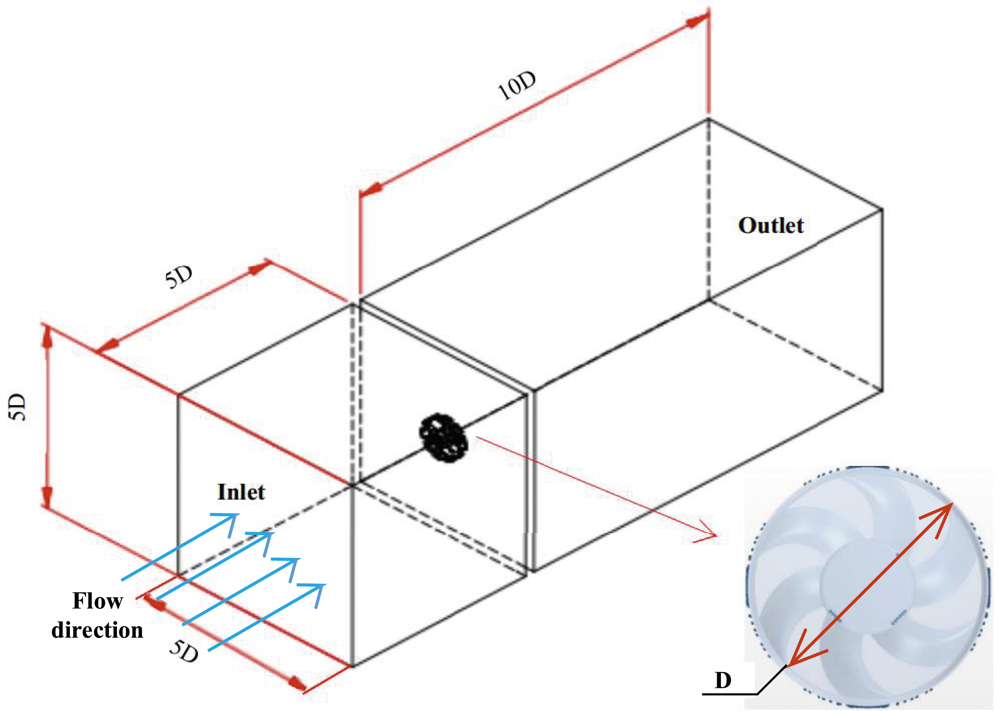
A reasonable geometrical aerodynamic model is an important foundation for numerical aeroacoustic prediction. The investigated model is a 6-blade automotive cooling fan module with a fan diameter of D = 31 cm. Figure 1(a) shows the original model of the fan and Figure 1(b) shows the fan test setup. The schematic of the computational domain is shown in Figure 2, where the numerical boundary conditions are indicated as well. Rotational and fixed domains are created in the numerical software. According to the aerodynamic test environment, the total length of the external fixed area is 2000 mm. The input and output are on the front and rear sides of the external fixed area, respectively. The boundary conditions at the inlet and outlet of the flow field are defined as the ambient pressure. Wall conditions are defined as “adiabatic, no-slip conditions.” As the Mach number of the flow is less than 0.2, the working fluid is defined as an incompressible gas.

Figure 1.

(a) The original model of the automobile fan, (b) the test setup of the fan together with the radiator.

Figure 2.

Computational domain and boundary conditions of the fan, where D is the diameter of the fan D = 31 cm.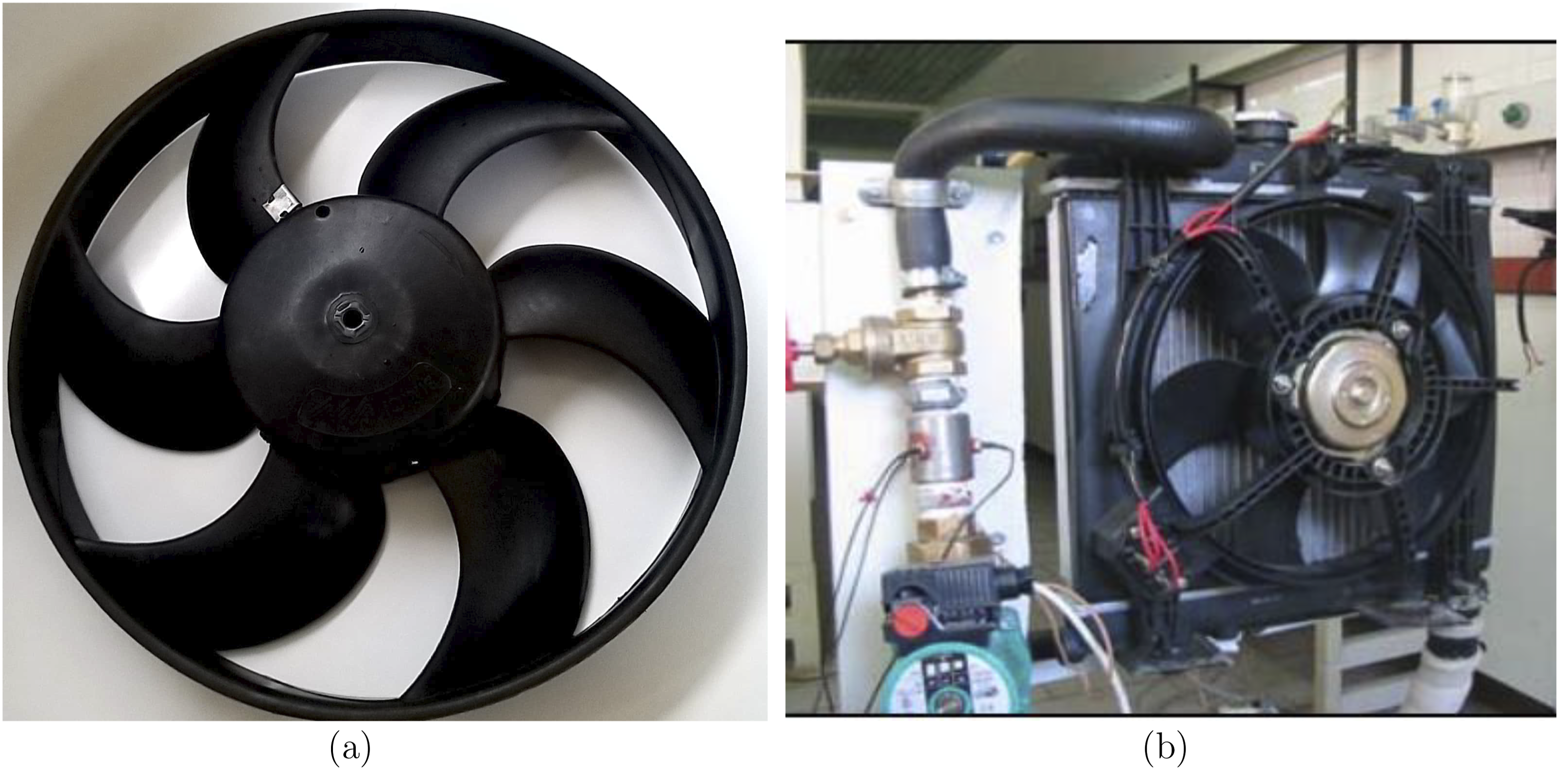

Mesh and boundary conditions

Due to the computational cost of running a DES simulation, creating an efficient grid is of key importance. Figure 3 shows the generated grid, where Figure 3(a) focuses on a cross-section of mesh distribution, Figure 3(b) presents a three-dimensional view, Figure 3(c) shows mesh on fan blades and Figure 3(d) shows mesh distribution in the entire computational domain. The computing area consists of two fixed and rotating parts. A polyhedral mesh is employed to solve the rotating area around the fan more accurately. In the rest of the domain, the trimmed mesh based on hexagonal elements is utilized. Naturally, in important flow areas, around the fan blade for example the mesh density is increased and in further areas where the flow is slower, the number of elements is decreased.

Figure 3.

Mesh distribution around the fan, (a) cross-section of mesh distribution, (b) three-dimensional view of the mesh distribution, (c) mesh distribution on fan blades, and (d) mesh distribution in the entire computational domain.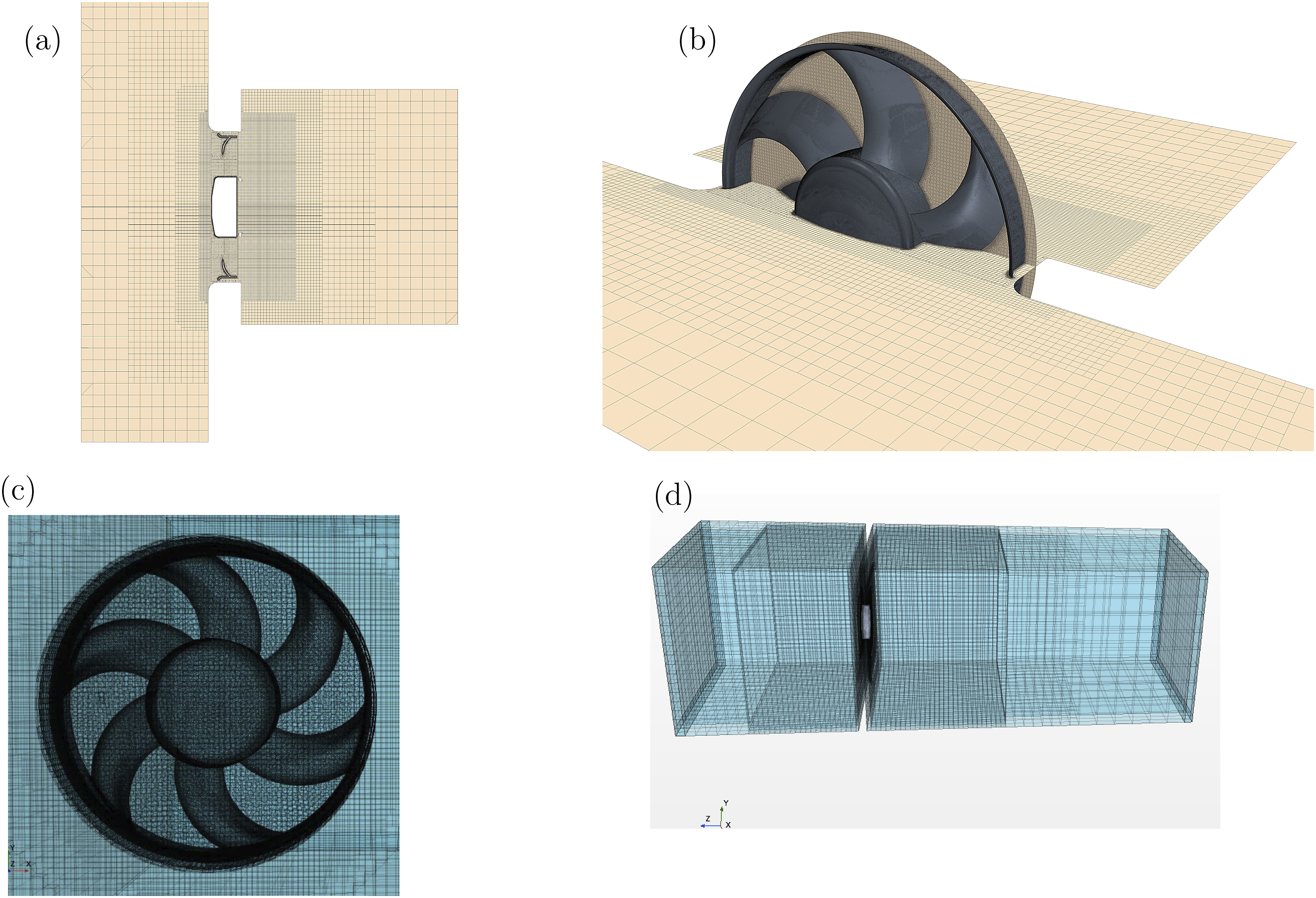

The inlet and outlet boundary conditions are considered in a way that distant effects and return flow do not affect the convergence of the solution. For the rotating area, the multiple rotating coordinate system method is used in the permanent mode. In this method, a rotating reference frame that is, a moving coordinate device is used for the area around the fan, and a fixed reference frame that is, a fixed coordinate device is used for the area outside the fan. In order to correctly predict the area near the wall, the number of layers in the boundary layer is equal to 10 layers and the distance of the first layer from the wall is 4 mm. In the simulation, the average value of the dimensionless distance from the wall is about y⁺ ≈ 2. Figure 4 shows the y⁺ value distribution on the fan blades. Figure 4(a) and (b) show the distribution of y⁺ on the suction and pressure side, respectively, which are suitable for the use of the turbulence model.

Figure 4.

The y⁺ value distribution on the fan blades. (a) The suction side; (b) the pressure side.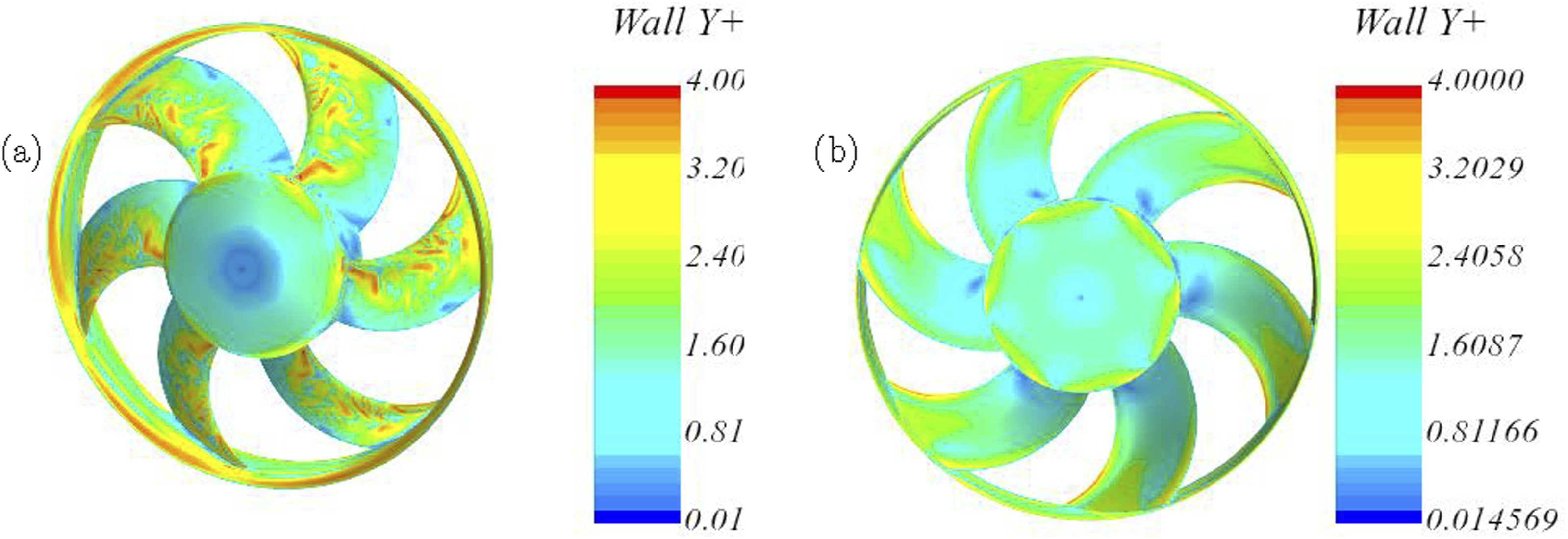

Grid independency and validation

Grid study

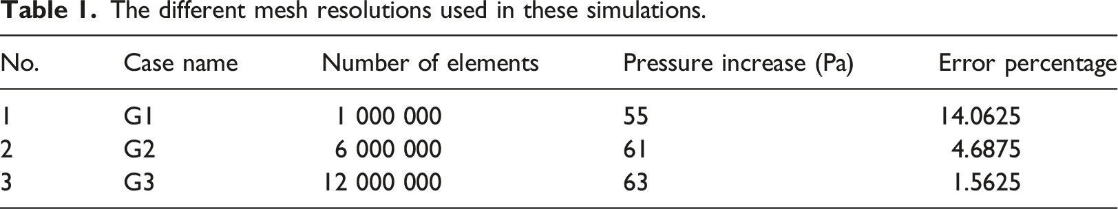
Figure 5 shows the number of elements with different quality levels for case G2. In Figure 5 the closer the quality value to unity, the higher the quality of the grid. As can be seen, the quality of many elements equals one and the rest have high quality and are appropriate. To investigate the sensitivity of the grid, three different mesh numbers of one million, six million, and 12 million are examined and named G1, G2, and G3 respectively. The rotating fan pressure is measured at the rotational speed of 1500 rpm using three different grid numbers. The values of pressure increase and the error stated in percentage are summarized in Table 1. These results are calculated with the k − ω turbulence model and the IDDES method, in an unsteady state, and with the time step of 0.000025 s.

Figure 5.

The cell quality diagram for the computational grid.

Table 1.

The different mesh resolutions used in these simulations.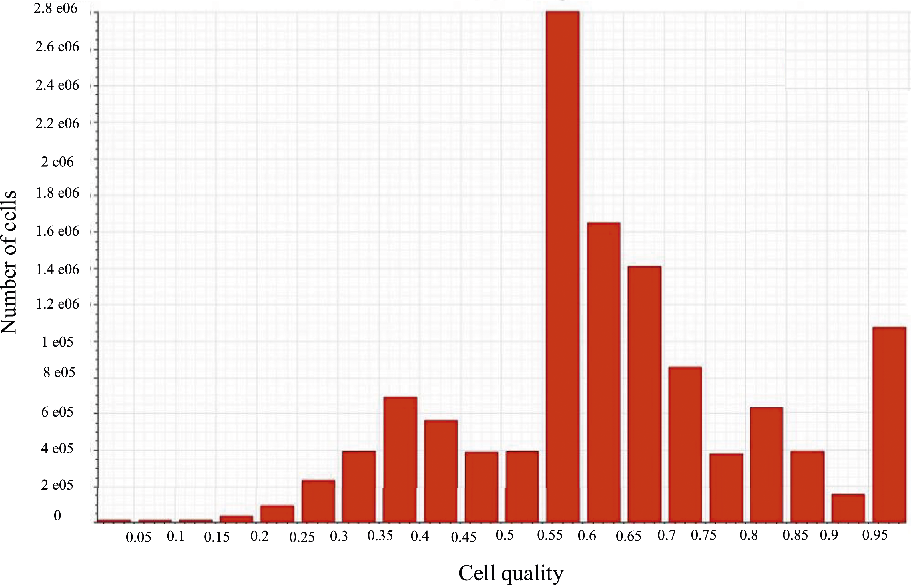

No.	Case name	Number of elements	Pressure increase (Pa)	Error percentage
1	G1	1 000 000	55	14.0625
2	G2	6 000 000	61	4.6875
3	G3	12 000 000	63	1.5625

Validation

In order to validate, single-blade fan simulation was performed by the RANS method for different mass flow rates at a rotational speed equal to 1500 rpm. The fan pressure was obtained at different mass flow rates and compared with the experimental measurements. It is found that the results of the numerical simulation are comparable with the experimental results. Figure 6 shows the variation of pressure rise with mass flow rate. The red line shows the result of the present study and the black line shows the experimental measurement. To measure and determine the fan characteristic curve experimentally, a fan test rig in accordance with the ANSI/AMCA 210-99 standard is used. The structure of the fan test setup is of the inlet chamber setup structure and the components of this rig include chambers, nets, nozzles, a variable discharge system, pressure measuring devices, and a data collection and processing system. Figure 1(b) shows the radiator and fan test setup. Upstream and downstream nozzle pressures are measured to determine airflow properties. Static and dynamic pressure are measured in different places and sent to the computer by DAQ card. The data received by the computer is extracted using the software and the characteristic curve including the static and the total pressures in terms of flow rate, is extracted. As is confirmed in Figure 6 the comparison is satisfactory.

Figure 6.

The pressure rise for different mass flow rates, line styles are as follows: : experimental measurement. : numerical simulation.

Arrangement of sound receivers and pressure probes

Figure 7(a) shows two probes that are used to monitor pressure in the numerical simulations while the solvers are running. The designated positions for locating the sound pressure receiver are situated within a 10 cm radius from the fan’s center. Additionally, there is a 7 cm separation from the fan’s disk plate both in the forward and backward directions. A total of 21 microphones are installed at specific locations. The location of the microphones on the azimuth plate is at a distance of 1, 2.5, and 4 m from the fan and with an angle difference of 30° degrees from each other. See Figure 7(b) for the arrangement of sound receivers. Please note that both sound receiver arrangements and pressure probe placements play a crucial role in capturing accurate acoustic measurements.

Figure 7.

The numerical arrangement of microphones at different angles and distances. (a) Probes location around the fan, (b) microphones location. Dimensions are in centimeters/meter.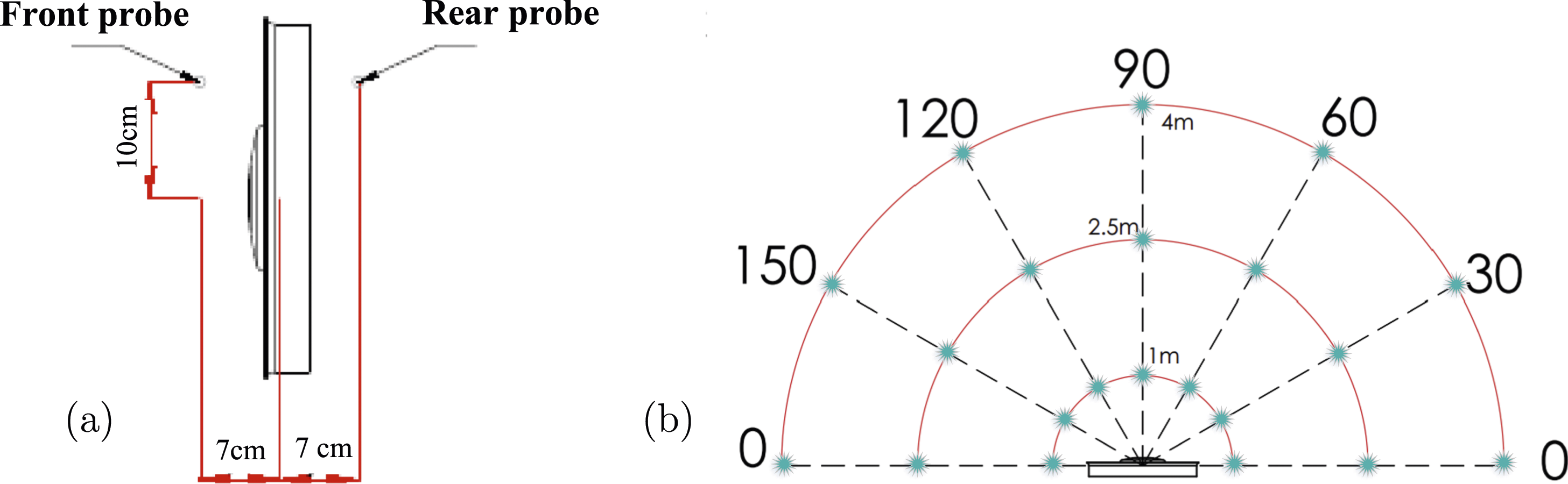

Noise experimental setup

For the verification of the noise prediction of the cooling fan, the noise experiment of the cooling fan is carried out. The noise experiment equipment is shown in Figure 8. The experimental test was conducted in a controlled laboratory environment. The fan, crucial to our measurements, was positioned at a specified height, and its rotational speed was meticulously controlled using a tachometer and power supply. Utilizing the B&K 3160 multichannel analyzer and a Type 2670 microphone ensured accurate and reliable measurements. The laboratory, with dimensions of 6 × 9 × 4 m, while not entirely sound-absorbing, is situated in an environment outside the city, minimizing noise pollution. Additionally, to further ensure the integrity of our results, all non-essential devices were deactivated during the testing phase. In addition, by measuring the background noise the standard requirements for an accurate test are fulfilled. Moreover, the turbulence intensity of the numerical simulations is set to be equal to that of the experimental value. The microphone position is the same as the receiving point in the numerical simulation, the test setup and microphone location are demonstrated in Figure 8. The experiment was performed at 1500 rpm for two angles of 0 and 90° degrees, and also at 2500 rpm for 90° degrees. In the 90° degree case, the fan’s sound was captured per the microphone manufacturer’s guidelines, without additional protection. Recorded data, spanning several seconds, underwent rigorous analysis with an emphasis on filtering out environmental noises for result accuracy.

Figure 8.

The noise experimental setup and related pieces of equipment.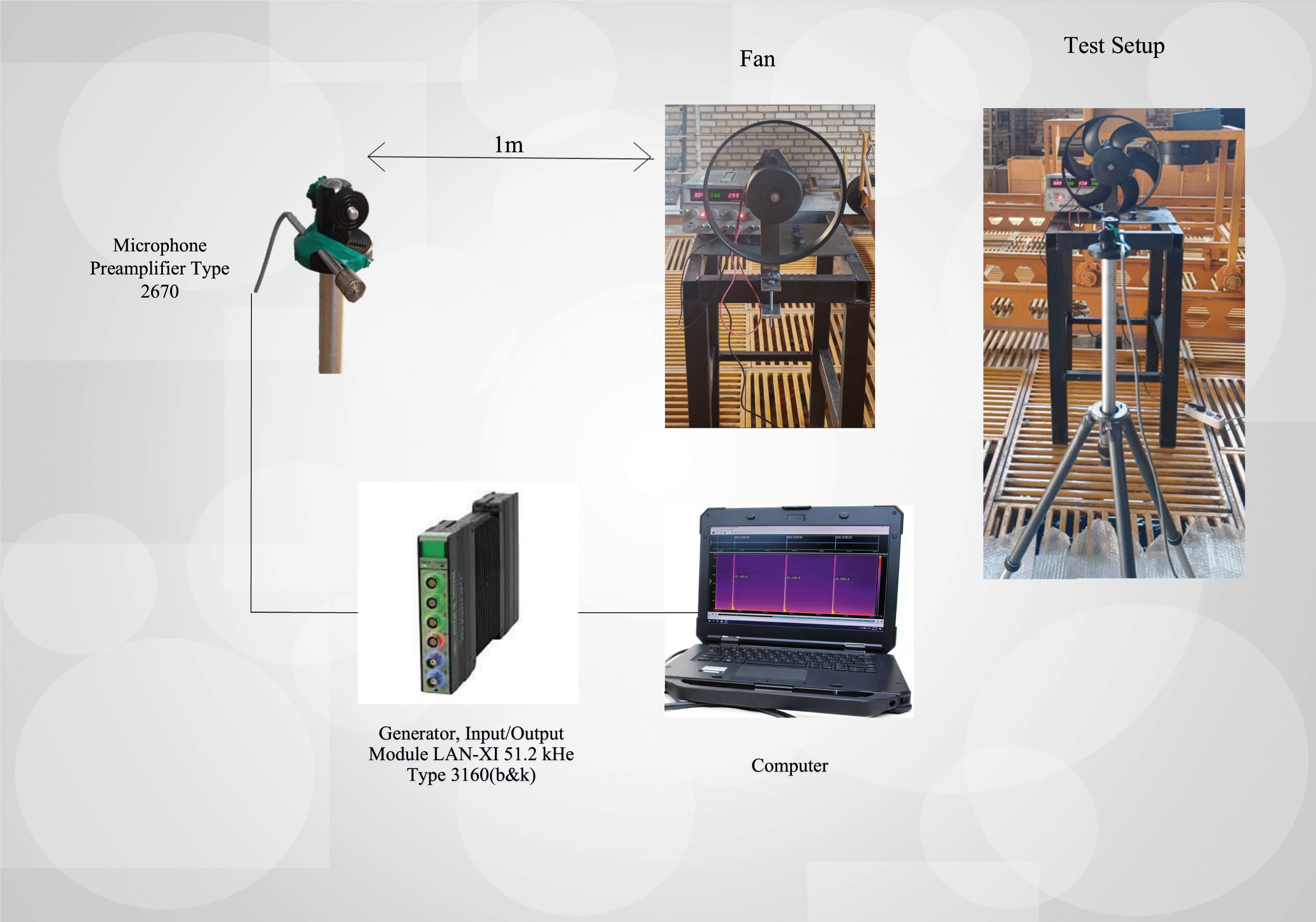

Variation of the sound pressure level at different frequencies for two rotational speeds 1500 and 2500 rpm is shown in Figure 9. The black and red lines show results of 1500 and 2500 rpm, respectively. Some main peaks and their harmonies can be seen in the figure, which can be calculated according to the rotational speed of its frequency. At the speed of 2500 rpm, a higher value was received at the peak of the graph.

Figure 9.

The experimental SPL diagram of the fan at 90° degree. Line styles are as follows: red and black lines show the results for the 1500 and 2500 rpm, respectively.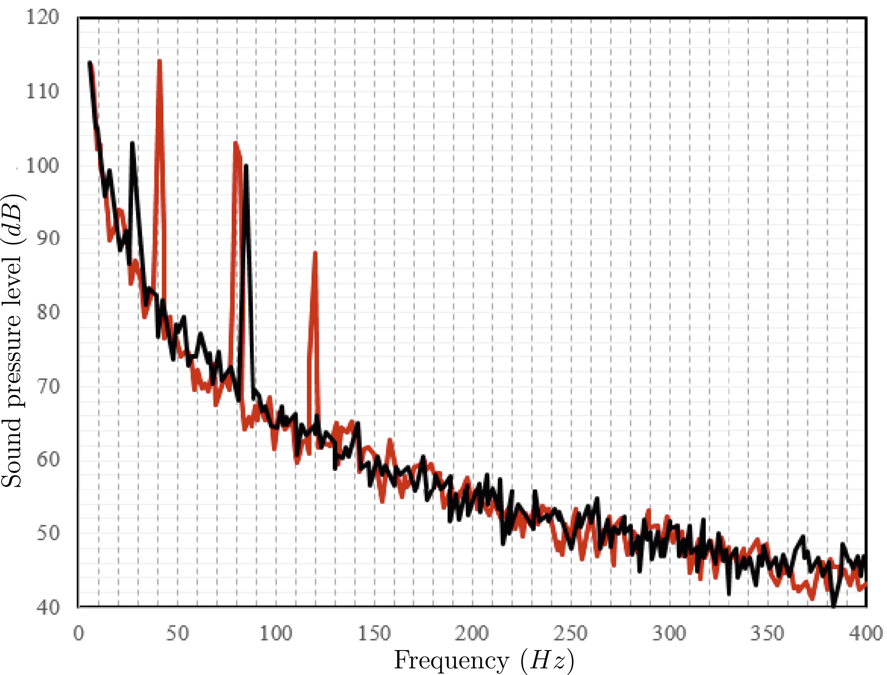

Figure 10 shows the measurement results variation of the sound pressure level at different frequencies for 0° and 90° degrees around the fan. The black and red lines show results of 90° and 0° degrees, respectively. In front of the hub that is, 90° degree, a higher value is received at the peak of the graph. There are several peaks in the graphs which could be due to interference between the rotating blades and shroud or other structural resonances.

Figure 10.

The experimental SPL diagram of the fan at 1500 rpm. Line styles are as follows: red and black lines show the results for the 0° and 90° degrees, respectively.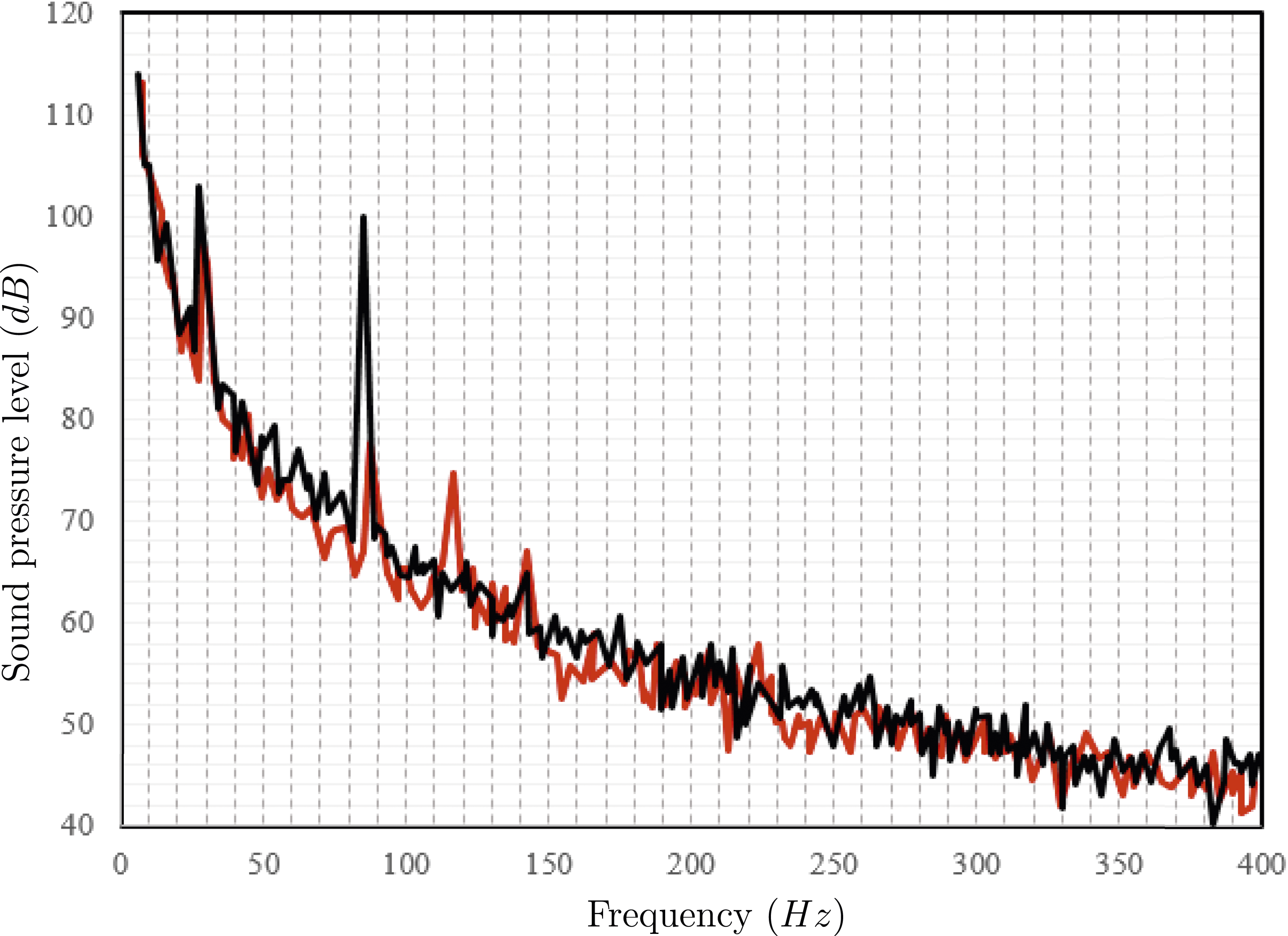

Results and discussion

Figure 11(a) and (b) show the pressure fluctuation field on the suction and pressure sides of the fan blades, respectively. As expected, the pressure on the suction side is lower than on the pressure side, and the highest pressure values are observed at the leading edge on the pressure side. The turbulent flow on the pressure side presents more significant fluctuations than those observed on the suction side. In addition, more significant interactions in the areas close to the trailing edge than the leading edge of the blades are observed. The aerodynamic noise is mainly generated by the interaction between the flow and the leading edges. As can be seen in Figure 11(a) the pressure field on the shroud surface is very inhomogeneous, which demonstrates that the shroud significantly affects the air distribution behind the fan blade surface. The interaction between the fan and the shroud leads to pressure fluctuation and vortex disturbance, which are considered the major source of the aerodynamic noise. Aerodynamic noise can be caused by the movement of turbulent flow or by the collision of aerodynamic forces with colliding surfaces.

Figure 11.

The numerical pressure field on the fan surface, (a) the suction side (b) the pressure side.

The contour plot of turbulent kinetic energy (TKE) on the surface of the fan is visualized in Figure 12. The distribution of TKE on the surface of a fan is closely related to the generation of noise. Areas on the fan’s surface with high TKE values correspond to regions where turbulence is more intense. In these high TKE zones, the velocity fluctuations are more pronounced, resulting in more significant variations in pressure and flow patterns. This, in turn, leads to the generation of stronger noise components. Naturally, high TKE regions can contribute to the formation of vortices, separation zones, and complex flow patterns near the fan blades. These flow features generate pressure fluctuations, which, when coupled with the solid surfaces of the blades, lead to the emission of aerodynamic noise. High TKE areas often lead to tonal noise components, characterized by distinct, repetitive frequencies. These tonal components are associated with the shedding of vortices and blade-passing frequencies. It can be seen in Figure 12 that as the distance from the root of the blade increases, the value of TKE increases as well. Hence, a logical deduction can be drawn that the elevated speed and more intense turbulence at the blade tips lead to higher values of kinetic energy within these specific regions. Additionally, according to Figure 12, the maximum amount of turbulent kinetic energy occurs at the tips of the blades on the leading edge. This can be attributed to the more intensified turbulence at the tips of the blades on the leading edge.

Figure 12.

The numerical contour plot of turbulence kinetic energy on fan surface.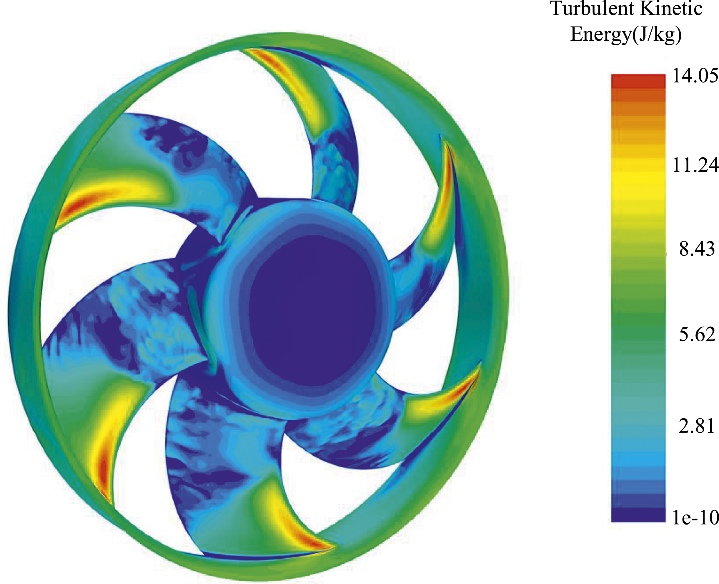

Analyzing the time history of acoustic pressure is crucial for understanding the noise generation and propagation characteristics of the fan. Figure 13 presents the variation of acoustic pressure over a specific duration of physical time. The x-axis represents physical time, in seconds, while the y-axis represents the acoustic pressure in pascals (Pa). The dashed red and solid black lines show the front and back probe results, respectively. The waveform exhibits oscillations that alternate between positive and negative values. The waveform’s amplitude corresponds to the magnitude of the acoustic pressure, indicating the strength of the sound wave at different points in time. For instance, a higher amplitude at around t = 0.03 s suggests a more intense sound, indicating a louder source. Peaks represent regions of maximum positive pressure, while troughs represent minimum negative pressure values. The distance between consecutive peaks or troughs represents the wavelength of the sound wave. The temporal pattern of the waveform can provide insights into the frequency and period of the sound wave. As shown in Figure 13, the pressure on the front side of the fan is higher than that of the backside. The span encompassing the observed changes as well as the degree of fluctuations detected collectively highlight the intrinsic non-uniformity characterizing both the fluctuations themselves and the predictive capability of the FW-H unsteady model. This dual observation suggests that the model possesses the capacity to anticipate such non-uniform fluctuations.

Figure 13.

The numerical time history of acoustics pressure. Line styles are as follows: dashed red and solid black lines show the results for the front and back probes, respectively.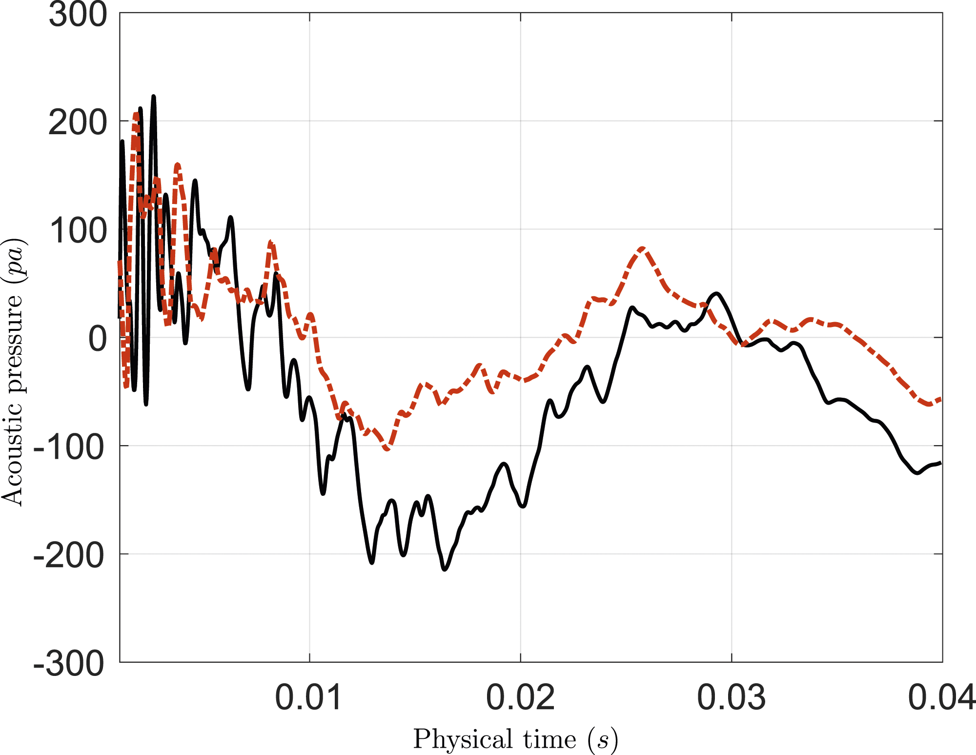

Analyzing the variation of the sound pressure level (SPL) at different frequencies of a fan provides valuable insights into its acoustic characteristics and noise generation mechanisms. Such an analysis helps identify dominant noise frequencies, harmonics, and overall noise profiles. Variation of the sound pressure level at different frequencies is plotted in Figure 14. The dashed red and solid black lines show the front and back probe results, respectively. The sound received via the front and back probes are almost comparable at most frequencies. However, higher sound pressure levels are detected with the back probe at some particular frequencies. The SPL of a fan exhibits a wide range of variation across different frequencies, providing insight into the acoustic characteristics and noise generation mechanisms associated with its operation. The sound pressure level varies between values around 130 dB to the very low values of about 30 dB at high frequencies. At the lower end of the frequency spectrum, the SPL of about 30 dB indicates relatively quiet periods. These low SPL values are often observed at high frequencies, which may be associated with minor mechanical vibrations or other noise sources that do not contribute significantly to the overall noise profile. On the other hand, as the frequency decreases and moves towards the midrange, the SPL starts to rise. This rise could be due to the interaction of the blades with the air generating noise through processes like blade-passing tones, vortex shedding, and turbulence. These mechanisms become more prominent in the mid-frequency range, leading to a gradual increase in SPL. The values around 60 to 80 dB in this midrange might indicate the dominant frequencies of these noise-generating processes. The peak of this graph is observed where the overall sound pressure level of the fan is about 115 dB at the frequency of 410 Hz. This specific frequency and SPL value can provide insights into the noise generation mechanisms and the fan’s acoustic profile.

Figure 14.

The numerical sound pressure level obtained from probes. Line styles are as follows: dashed red and solid black lines show the results for the front and back probes, respectively.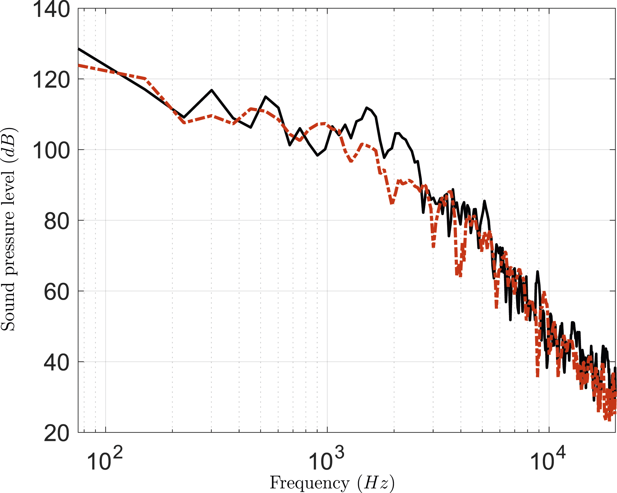

Figure 15 depicts the acoustic power contours of the fan, which have been generated utilizing receiver data collected at a distance of 1 m and various angles including 0°, 30°, 60°, and 90° degrees. These contours provide a comprehensive understanding of how the fan’s noise emission varies across different angular positions. As is observed in Figure 15(a), at 0° degrees, representing the frontal orientation, the contour reveals the primary noise sources directly in line with the fan’s rotation. According to Figure 15(b)–(d), moving to 30° degrees, the contour gains higher values. However, at 60° degrees much higher values are observed, which are comparable to the highest amount of noise that is received at an angle of 90° degrees. As can be seen in Figure 15 in all receivers, the highest amount of noise is produced at the tip of the blades. In addition, the lowest amount of noise is produced at the root of the blades, which also has the lowest linear velocity. As shown previously in Figure 12, the kinetic energy of turbulence has the highest value in these areas. On all blades, the amount of noise decreases by moving from the leading edge to the trailing edge. Collectively, these acoustic power contours provide a comprehensive visualization of the fan’s noise profile, offering valuable insights into its acoustic behavior from different angles and aiding in targeted noise mitigation strategies for the automotive application.

Figure 15.

The numerical acoustic power contour, (a) 0° degree from fan, (b) 30° degree from fan, (c) 60° degree from fan and (d) 90° degree from fan.

Figure 16 shows the overall sound pressure level OSPL plot of the fan at different microphone locations. The OSPL prediction of the fan has been performed at a distance of 1 m upstream from the fan inlet. The highest value is observed at 90° degree angle and is equal to 87.9 dB and the lowest value is observed at 0° degree angle and is equal to 72.3 dB. This image offers insights into the fan’s directivity characteristics and its contribution to the overall sound pressure level. Evidently, the most prominent noise emissions are discernible at a 90° degree angle, a finding that aligns with the patterns observed in Figure 15. However, as can be seen in Figure 16 the sound around the fan is propagated polarly.

Figure 16.

The numerical overall sound pressure level around the fan at the 1 m distance in front of the fan.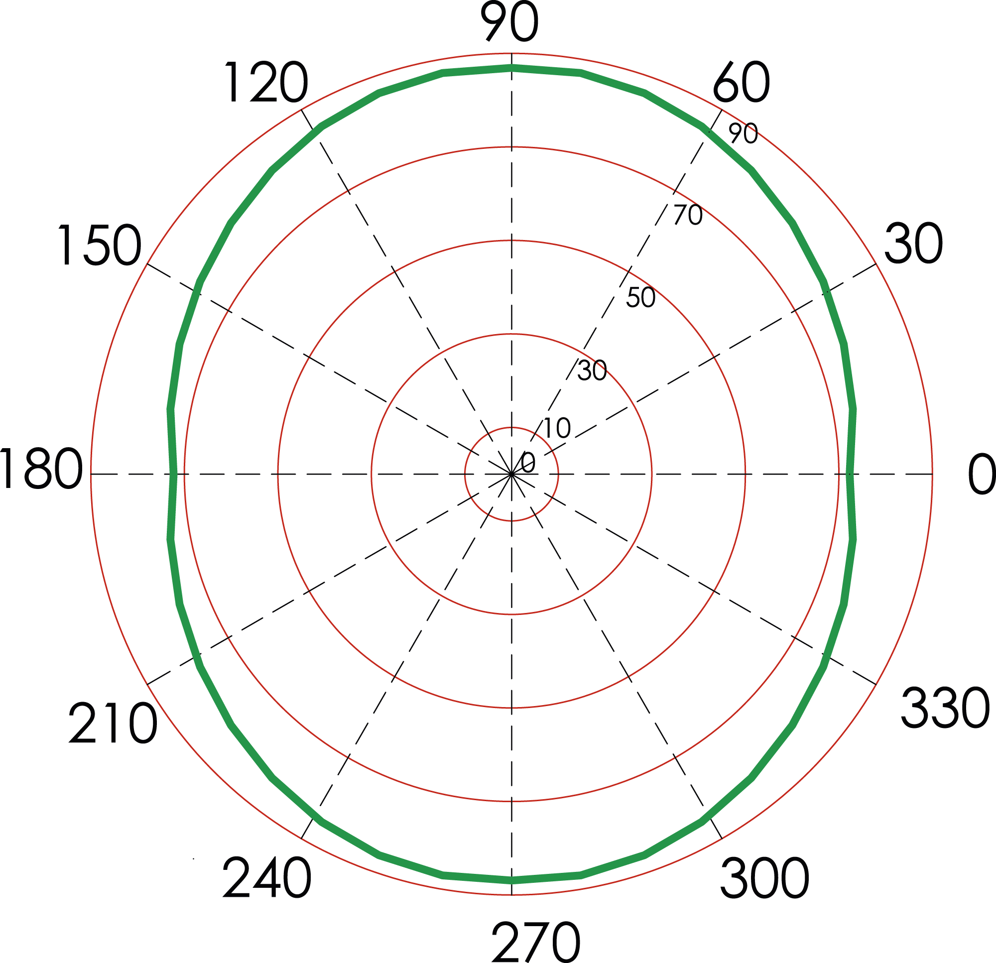

Figure 17 shows the sound pressure level diagram in different receivers. These diagrams are plotted for receivers located at distances of 1 and 2.5 m from the fan. Line styles are as follows: dotted red, dash-dotted black, dashed blue, and solid green lines indicate 90°, 60°, 30°, and 0° degrees, respectively. Considering Figure 17 it is observed that the tonal noise is predominant at low frequencies that is, below 1000 Hz, and a maximum is observed at 500 Hz. According to the SPL diagram of the fan, the maximum amount of noise is at a 90° degree angle and when approaching the side angles, the less the fan noise becomes, and the minimum amount of noise is at angles of 0° and 180° degrees.

Figure 17.

The numerical SPL diagram of the fan at (a) radius = 1 m and (b) radius = 2.5 m from the fan. Line styles are as follows: dotted red: 90° degree, dash-dotted black: 60° and 120° degrees, dashed blue: 30° and 150°, solid green: 0° and 180° degrees, respectively.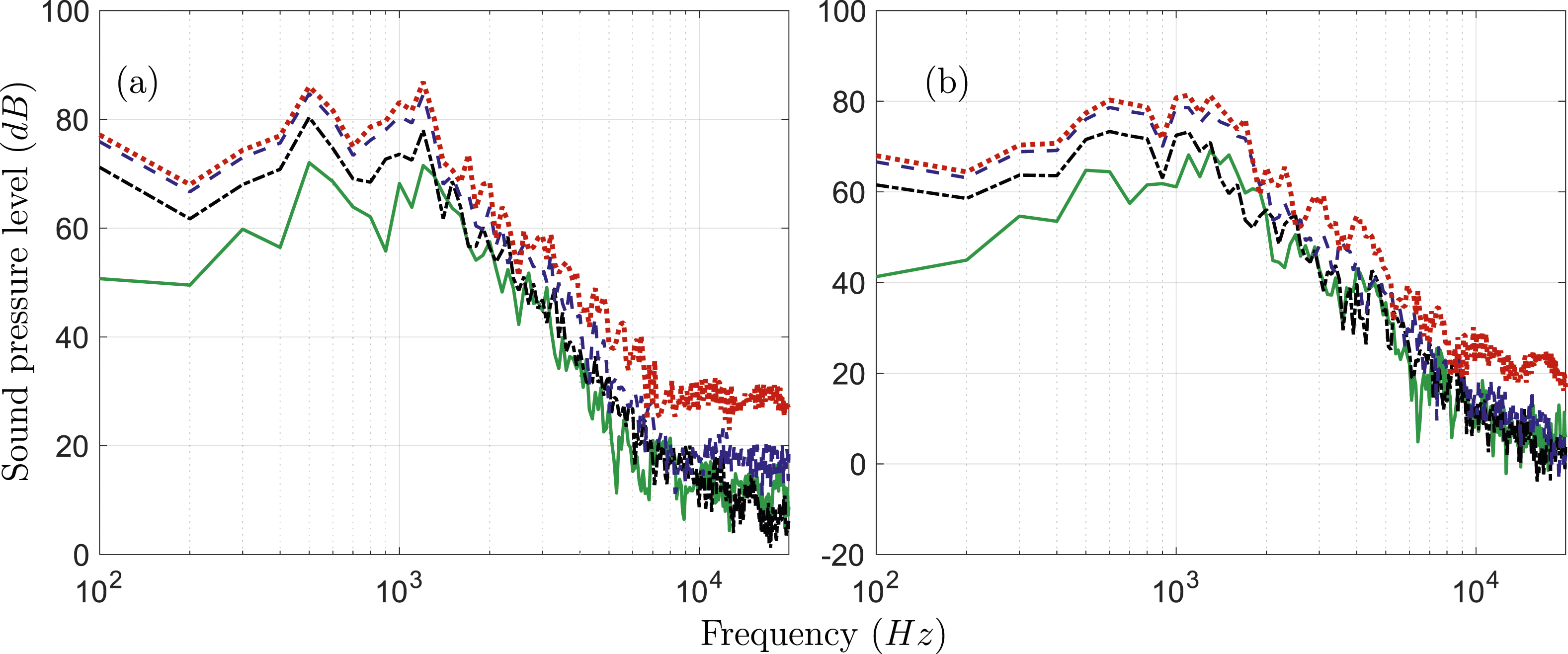

Figure 18 shows the sound pressure level diagram in relation to the frequency at the angle of 90° degree and at different distances from the fan. The dashed blue, dash-dotted black, and solid green lines represent the results of the receiver at radial distances of 1 m meters, 2.5 m meters, and 4 m meters, respectively. As expected, the highest sound pressure level received is related to the microphone placed at a distance of 1 m. As the distance from the fan increases, the received sound is observed to be at a lower level. The trend is almost the same at all frequencies.

Figure 18.

The numerical SPL diagram of the fan at 90° degree from fan. Line styles are follows: dashed blue: radius = 1 m, dash-dotted black radius = 2.5 m and solid green: radius = 4 m.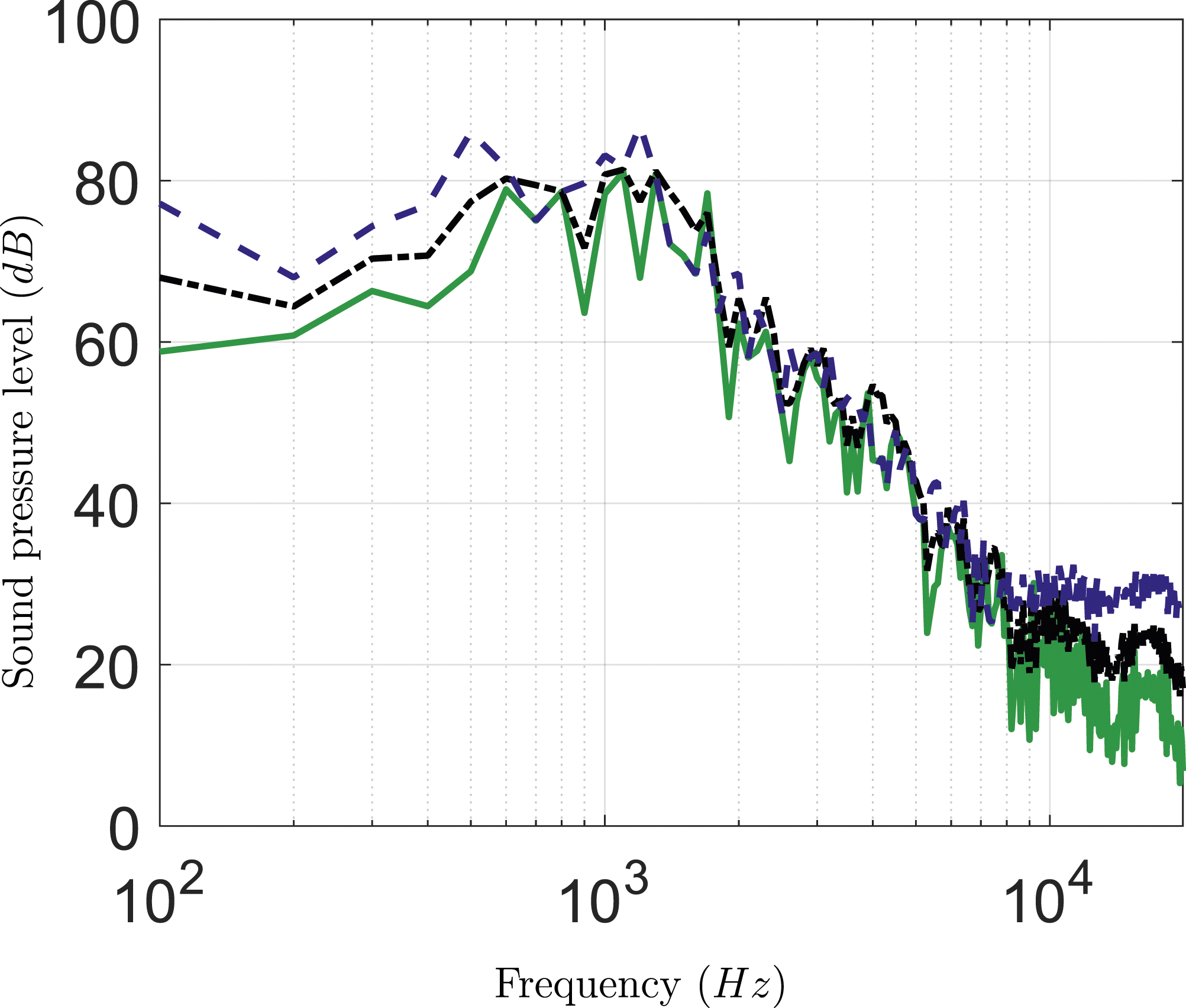

Figure 19 reveals the results of both numerical simulation and experimental testing under the same conditions, specifically at 1500 rpm and 90° degrees. Generally, the numerical simulation indicates a lower value, attributed to factors such as test conditions, environmental noise, and wall reflections, which are absent in the numerical simulation. Despite these variations, the distinctive tonal noise evident in the experimental test is similarly observed in the numerical simulation, albeit with a minor difference in the corresponding frequency range.

Figure 19.

The experimental and numerical SPL diagram of the fan at 1500 rpm and 90° degree. Line styles are as follows: dashed red and solid black lines show the experimental and numerical results, respectively.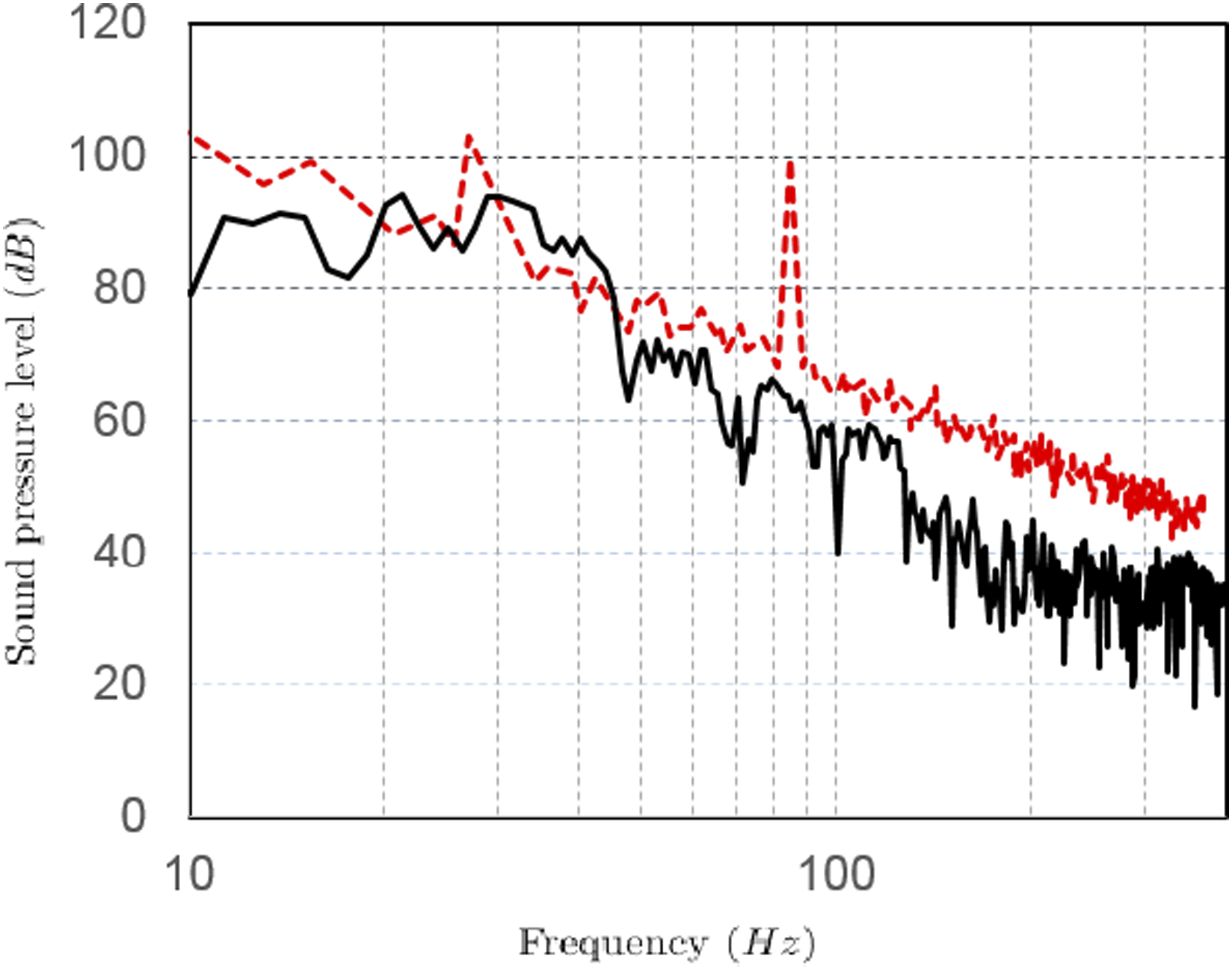

Summary and concluding remarks

The present study examined a cooling fan module both experimentally and numerically. To measure and determine the fan characteristic curve experimentally, the pressure rises for different mass flow rates are obtained using a fan test rig. The corresponding experimental results are comparable with the numerical outcome. In addition, the noise experiment of the cooling fan is carried out. The experimental results of the SPL for two rotational speeds 1500 and 2500 rpm are assessed and at 1500 rpm for two angles of 0° and 90° degrees around the fan, SPL at different frequencies is evaluated.

To perform the numerical investigation, a CFD model is utilized using DES to capture fan noise source information. The sound pressure level of the fan in working conditions is extracted and compared with experimental results, and its independence from the numerical grid and its uncertainty are investigated. The results of this analysis are in good agreement with the results of the experimental test, which indicates the appropriate accuracy of the meshing and solver conditions. It is observed that the DES model predicts noise well. This study showed that the noise produced by the fan is relatively different due to the combination of several noise sources; namely: (i) The interaction of the fan blade with the collision of the turbulent flow and the boundary layer. (ii) Noise behind the blade due to the development and separation of the turbulent boundary layer. (iii) Vortex noise related to the von Kármán vortices that is, circulating release. (iv) Noise generated by diffuse currents and tip vortices.

The simulation results showed that the sound pressure level at the entrance is higher than at the exit. Tonal sound is the main component of aerodynamic sound. It is observed that the sound field has a strong axial dipole characteristic at low frequencies while axial deviation occurs at high frequencies. Moreover, in the investigations, it was observed that the pressure field on the shroud surface is very inhomogeneous, which demonstrates that the shroud significantly affects the air distribution behind the fan blade surface. Additionally, The TKE analysis reveals that as the distance from the root of the blade increases, the value of TKE increases which can be attributed to the higher speed and more intensity of turbulence at the tips of the blades.

The time history of acoustic pressure and the sound received via the probes in front and back of the fan is inspected. Insight into the fan’s directivity characteristics is gained with an examination of the overall sound pressure level. In particular, higher sound pressure levels are detected with the back probe at some particular frequencies. The peak is observed where the overall sound pressure level of the fan is about 115 dB at the frequency of 410 Hz. Remarkably, it is observed that the tonal noise is predominant at low frequencies that is, below 1000 Hz, and a maximum is observed at 500 Hz. Furthermore, it is observed that at a certain distance from the receiver, the tonal noise and the bandwidth noise increase with the rotational speed. By interpreting the experiment and simulation results, it is concluded that the maximum amount of noise is at the angle of 90° degrees and the sound pressure level does not change much from a distance of 1 to 2.5 m.