Extension of the concept of Ffowcs-Williams and Hawkings type wave extrapolation to non-trivial flow effects and exterior surfaces

Abstract

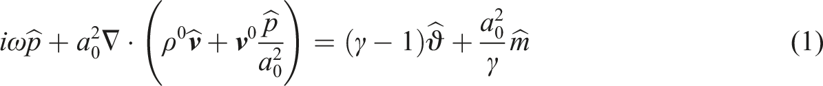
In appreciation of Ffowcs-Williams and Hawkings’ seminal contribution on describing the sound radiation from moving objects, this article discusses a concept of taking into account local non-trivial flow effects on the sound propagation. The approach is motivated by the fact that the numerical simulation of the sound propagation from complete full scale aircraft by means of volume-discretizing (CAA = Computational AeroAcoustics) methods is prohibitively expensive. In fact, a homogeneous use of such CAA approach would waste computational resources since for low speed conditions the sound propagation around the aircraft is subject to very mild flow effects almost everywhere and may be treated by more inexpensive methods. The part of the domain, where the sound propagation is subject to strong flow effects and thus requiring the use of CAA is quite restricted. These circumstances may be exploited given a consistent coupling of methods.

The proposed concept is based on the strong (alternatively weak) coupling of a volume discretizing solver for the Acoustic Perturbation Equations (APE) and a modified Ffowcs-Williams and Hawkings (FW-H) type acoustic integral. The approach is established in the frequency domain and requires two basic ingredients, namely a) a volume discretizing solver for the APE, or for Möhring-Howe’s aeroacoustic analogy, to take into account strong non trivial flow effects like refraction at shear flows wherever necessary, and b) an aeroacoustic integral equation for the propagation part in areas where non-potential mean flow effects are negligible. The coupling of this aeroacoustic integral and the APE solver may be realized in a strong (i.e. two-ways) form in which both components feed back information into one another, or in a weak form (i.e. one-way), in which the sound field output data from the APE solver serves as given input for the integral equation. If an aircraft geometry has minor influence on the sound radiation to arbitrary observer positions, the aeroacoustic integrals may simply be evaluated explicitly. If on the other hand, the presence of the geometry has an important influence on the sound radiation, then the acoustic integral equation is implicit and requires some sort of numerical solution, in this case a Fast Multipole Boundary Element solver. While conceptually the weak coupling follows the spirit of the FW-H approach to describe sound propagation from aeroacoustic sources the underlying aeroacoustic integral is not based on Lighthill’s analogy, but the aeroacoustic analogy of Möhring-Howe. This is a consequence of the fact that in the two way-coupling the acoustic particle velocity in a moving medium needs to be determined, which is non-trivial based on an acoustic integral. As an important feature of the strong coupling the acoustic integral also provides practically perfect non-reflection boundary conditions even when the desireably small CAA domain does not extend into the far field. The validity of the presented computation approach is demonstrated in two example use cases.

Introduction

The installation of propulsors, may it be turbofans, or propellers, on the aircraft may alter their sound radiation considerably. Two main effects come into the picture: (a) source effects and (b) radiation effects. An example for (a) would be a non-uniform inflow condition to a turbofan due to tight engine airframe integration with extreme cases like boundary layer ingestion (BLI). In the context of propeller installation sources the excess noise of pusher arrangements downstream a wing could be mentioned. In both cases the rotating blades experience unsteady loading as they move through the flow inhomogeneities. Apart from this source effect the installation may also affect the acoustic radiation (b) considerably, once the sound has been generated. The radiation-wise installation effects in turn subdivide into two mechanisms, which generally occur in combination. On the one hand the local flow field surrounding the source may have a strong influence on the propagation due to convection, refraction and scattering; on the other hand the acoustic radiation is subject to reflection, diffraction at (hard) surfaces. This article is focused on providing a very efficient computation approach, which allows to take into account the effect of the complete aircraft geometry including all relevant flow effects on the sound radiation of a given source (typically the engine) attached to the aircraft.

Problem background

In general it is important to be able to include the complete aircraft surface in the description of acoustic installation effects of a sound source, e.g. the fan or propeller. Volume resolving discretization schemes to solve the Linearized Euler Equations (LEE) or Acoustic Perturbation Equations (APE) typically all involve high computational complexity and could be substituted by more computationally efficient methods for most day-to-day applications. Ray tracing approaches on the other hand are super efficient but may oversimplify e.g. the situation of acoustic shielding because of problems with representing the diffraction properly or representing extended sources of sound. A view on the problem shows that strong flow effects, which require the use of full blown (volume discretizing) Computational AeroAcoustics (CAA) methods, are typically restricted to quite small sized sub domains, e.g. the intake and intake duct of a turbofan, see e.g. the areas in Figure 1 sketched in green. Most of the domain around the aircraft body however, is subject to flow which is potential or even almost uniform, where very efficient acoustic integral methods are sufficiently accurate, e.g. the surfaces inside the blue lines in Figure 1. Therefore one natural choice would be an appropriate combination of these two approaches in a way as to exploit their respective pros while avoiding the cons.

Figure 1.

Typical problem arrangement of wing or rear installed propulsors on aircraft (upper part turbofan, lower part propeller). Green volumes represent 3D (APE) computation domains, while blue lines indicated 2D (BEM) surface areas which influence the sound radiation due to the aircraft’s surface. The red lines indicate that within this computation concept rotors under installation conditions could potentially be represented by body force models derived from an actuator disk RANS solution of the flow field and driving the 3D perturbation solver Dierke ⁶ ; Franco. ⁷

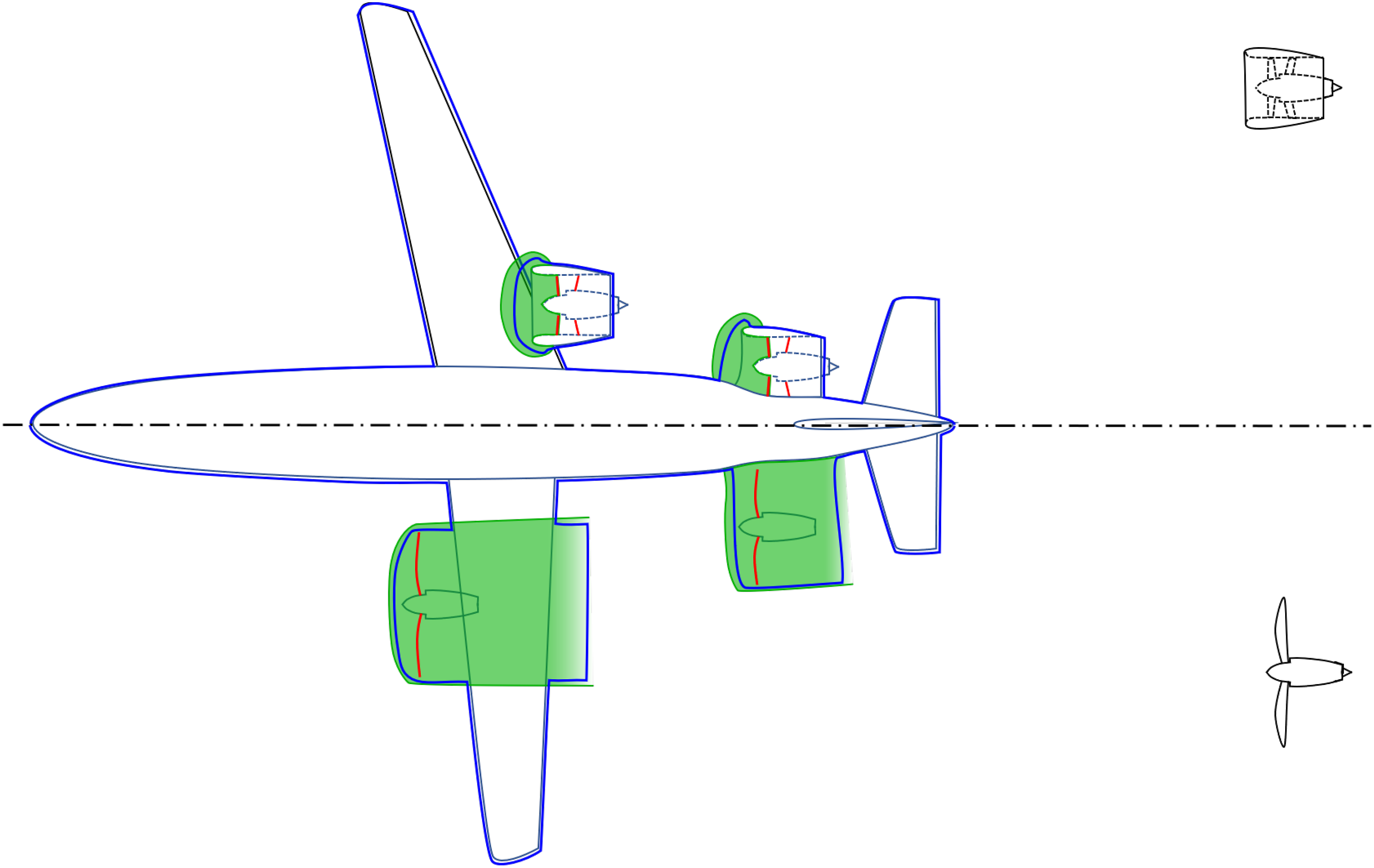
The key question here is the appropriate choice of subdomains for the volume resolving part and the surface integral part and to find a way to couple these consistently. One important issue is, that upon minimizing the subdomain in which the (expensive) 3D perturbation solver works, its free boundary will be located in the nearfield, where local non-reflection boundary conditions (NRBCs) are typically inaccurate. Therefore the coupling with the surface integral solver has to provide for a clean radiation condition in a situation where non radiating signal components are present and radiation components will hit the free boundary at very shallow angles etc. In this context, the availability of not only the sound pressure, but the acoustic particle velocity $\widehat{\mathit{v}}$ as an input to the free boundary of the 3D perturbation solver is a central issue in the two-way coupling. With flow present it is not straight forward to determine $\widehat{\mathit{v}}$ even if $\widehat{p}$ is known from a Ffowcs-Williams and Hawkings (FW-H) acoustic integral.

One solution is to let the respective acoustic integral be based on Möhring-Howe’s acoustic analogy rather than the one of Lighthill’s. Following this path, and assuming uniform flow outside the integral surface, Heitmann et al. ⁸ derived a FW-H type sound field prediction for the stagnation enthalpy $\widehat{B}$ as the acoustic variable, from which the sound pressure as well as the particle velocity and any other related variable like sound intensity and sound power may be obtained (even in the nearfield). The same approach was applied in Dürrwächter et al. ⁹ and Dürrwächter ¹⁰ for the prediction of the sound radiation from a rear-fuselage installed contra rotating propeller at flight conditions including the acoustic influence of the rear fuselage surface. Casenave et al. ¹¹ realized a coupling between a boundary integral method with a FEM solver in uniform flow for the sound scattering at a cylinder in potential cross flow. Proskurov et al. ¹² consequently coupled a Discontinuous Galerkin volume resolving code to solve the acoustic perturbation equations (APE) ¹³ for sound propagation in non-uniform flow with a fast multipole multidomain boundary element solver for the Helmholtz equation, derived from the Taylor transform of Möhring’s wave equation.

Method

The proposed methodology for computing the sound radiation of installed engines at complete aircraft is a useful new combination of established methods, which have been validated and published separately before. Upon coupling them in an appropriate way complex local flow related propagation effects may be accurately accounted for while taking into account the effect of the complete actual aircraft geometry on the sound radiation in parallel. The purpose of this (strong) coupling of methods is to reach a particularly high computational efficiency required when acoustic predictions are desired for full scale aircraft at high geometric fidelity. One particular difficulty with installation effects is their non generic nature, i.e. in contrast to aeroacoustic aircraft component source noise models the (aero)acoustic installation conditions of a propulsor is typically highly specific, so generic empiric or analytical models for the description of installation effects cannot really be provided.

There are three main components of this computational approach, namely

(i) Volume resolving CAA perturbation solver for the APE or LEE (in this case the DLR inhouse 4th order Discontinuous Galerkin solver DISCO++) ¹⁴

(ii) Surface resolving BEM convective wave equation solver, formulated for the computation of pressure and acoustic particle velocity (in this case the DLR inhouse fast multipole multidomain BEM solver FMCAS) ¹⁵

(iii) interface equations for the coupling of CAA DG and BEM acoustic integral equation solver

The DG code was chosen since it works on unstructured (tetrahedral) grid cells, which enable a comparatively simple mesh generation even for complex 3D geometries. A frequency domain version of the DG solver is needed to enable the (strong) coupling to the BEM solver FMCAS, which for the purpose of exploiting the required fast multipole acceleration is formulated in the frequency domain. Last but not less important is the problem that in the two way coupling between CAA and BEM not only the sound pressure $\widehat{p}$ needs to be provided on the free boundary of the DG solver, but also the particle velocity $\widehat{\mathit{v}}$ .

In what follows, the main components of the proposed methodology are briefly described. For details on any of these, the reader is referred to respective publications ¹² Here, focus is put on the overall coupled approach and the necessary steps.

Volume discretizing solver for the solution of the APE

For the prediction of the sound propagation under complex flow conditions (for instance the subdomains in Figure 1) sketched in green) the DLR inhouse code DISCO++ is used in a variant which solves numerically the APE in the frequency domain

$i\omega \widehat{p}+a_0^2\mathit{\nabla }\cdot \left({\rho }^0\widehat{\mathit{v}}+{\mathit{v}}^0\frac{\widehat{p}}{a_0^2}\right)=\left(\gamma -1\right)\widehat{\vartheta }+\frac{a_0^2}{\gamma }\widehat{m}$

(1)

$i\omega \widehat{\mathit{v}}+\mathit{\nabla }\left({\mathit{v}}^0\cdot \widehat{\mathit{v}}+\frac{\widehat{p}}{{\rho }^0}\right)=\frac{1}{{\rho }^0}\widehat{\mathit{f}}\cdot$

(2)

Here, p represents pressure, and v the velocity vector, ρ the density, a the speed of sound; a superscript 0 indicates the given mean flow, while the hat symbol indicates the complex amplitude $\widehat{\varphi }\left(\mathit{x},\omega \right)=\frac{\omega }{2\pi }{\displaystyle {\int }_0^{2\pi /\omega }\varphi \prime }\left(\mathit{x},t\right)\exp \left(-i\omega t\right)dt$ of a fluctuating quantity ϕ^′, t being time, x location and ω the considered angular frequency. The isentropic exponent is denoted γ. The (given) excitation source terms for heat, mass and momentum are denoted $\widehat{\vartheta }$ , $\widehat{m}$ and $\widehat{\mathit{f}}$ respectively.

DISCO++ employs a Discontinuous Galerkin discretization of the field into tetrahedral elements. Orginally formulated as a time domain code which the iteration to the steady monochromatic solution is accomplished in a most straight forward manner using pseudo time stepping with again the available RK4 scheme.

Apart from sources in the volume (e.g. given rotating body forces to represent propeller blades) also incoming, given sound fields may be specified at parts of the boundaries, e.g. upstream traveling duct modes in the outflow domain boundary inside a duct ^{14 2}

Surface discretizing solver for the solution of the convective wave equation

The DLR inhouse code FMCAS is a boundary element method formulated in the frequency domain for the solution of the Helmholtz equation; it employs the fast multipole algorithm in a multiple domain implementation for computational acceleration. The presence of a flow is taken into account by use of Taylor’s transform to map a convected wave equation onto the Helmholtz equation before the latter is solved numerically. The basis for a surface integral equation for acoustics is some wave equation. Since the coupling interface to the APE-domain is typically located in areas with flow an appropriate wave equation has to be chosen. In what follows, no volume source is assumed present at this interface. An acoustic wave equation which may describe such situation exactly for potential mean flows is Möhring-Howe’s analogy equation using the perturbation of the stagnation enthalpy

$\widehat{B}=\frac{1}{{\rho }^0}\widehat{p}+{\mathit{v}}^0\cdot \widehat{\mathit{v}}$

(3)

as the acoustic variable. Note, that by using equation (2) in its homogeneous form the particle velocity may be determined from $\widehat{B}$ like

$\widehat{\mathit{v}}=-\frac{1}{i\omega }\mathit{\nabla }\widehat{B}$

(4)

and the sound pressure $\widehat{p}$ is then retrieved by means of (3). Möhring-Howe’s equation ¹⁶ is exact for potential flows and reads

$\left(i\omega +{\mathit{v}}^0\cdot \mathit{\nabla }\right)\left[\frac{1}{a_0^2}\left(i\omega \widehat{B}+{\mathit{v}}^0\cdot \mathit{\nabla }\widehat{B}\right)\right]-\frac{1}{{\rho }^0}\mathit{\nabla }\cdot \left({\rho }^0\mathit{\nabla }\widehat{B}\right)=0$

(5)

Equation (5) is a direct consequence of equations (1) and (2) and equation (3) and insofar they are compatible to one another. The drawback of Möhring-Howe’s equation as it stands, is, that no generally valid Green’s function is available. However, Taylor’s transform ¹⁷

$\tilde{\mathit{\nabla }}=\mathit{\nabla }-i\omega \frac{{\mathit{v}}^0}{a_0^2}$

(6)

may be applied to substitute ∇ in Möhring-Howe’s wave operator from (5) for this step will reduce it to the classical wave operator in the transformed space (denoted with a tilde symbol) at least up to terms quadratic in the flow Mach number M = | M | = | v ⁰/a₀| and mild gradients of it (see the higher order terms in Appendix)

$\frac{{\omega }^2}{a_0^2}\widehat{B}+{\tilde{\mathit{\nabla }}}^2\widehat{B}\simeq 0.$

(7)

Taylor’s ansatz for $\widehat{B}$ to explicitly take into account the respective convection correction for an assumed potential background flow with Mach numbers much smaller than unity and mild gradients is

$\widehat{B}=\tilde{B}T,\text{with}\mathrm{ }T=\exp \left(i\frac{\omega }{a_0^2}{\varphi }^0\right)$

(8)

Here, ϕ⁰ represents the potential of the (steady) background flow v ⁰ = ∇ ϕ⁰. Inserting (8) into Möhring-Howe’s equation (5) will reduce it to the classical wave operator just as (7) and with exactly the same higher order terms in the Mach number (as in (13)), but now in orginal coordinates. Furthermore, again up to second order in the Mach number, the local speed of sound a₀ may be replaced by its value in the freestream a _∞ (see Appendix)

$k^2\tilde{B}+{\mathit{\nabla }}^2\tilde{B}\simeq 0,\text{with}\mathrm{ }k=\frac{\omega }{a_{\infty }}$

(9)

Once the solution for $\tilde{B}$ has been determined (8) is used to obtain the stagnation enthalpy $\widehat{B}$ as needed.

Thanks to the availability of the free field Green’s function ${\tilde{G}}_0\left(\mathit{x},\mathit{\xi }\right)=\exp \left(-ikr\right)/\left(4\pi r\right)$ , r = | x − ξ |, for $-\left(k^2+\mathrm{\Delta }\right){\tilde{G}}_0=\delta \left(\mathit{x}-\mathit{\xi }\right)$ the problem of solving for the acoustic field in the exterior to a closed surface S = S _B + S _F may be recast into the integral equation

$\alpha \left(\mathit{x}\right)\tilde{B}\left(\mathit{x},\omega \right)={\displaystyle \underset{S_F}{\int }\tilde{B}\left(\mathit{\xi }\right)}\frac{\partial {\tilde{G}}_0}{\partial n}-G_0\frac{\partial \tilde{B}}{\partial n}dS\left(\mathit{\xi }\right)+{\displaystyle \underset{S_B}{\int }\tilde{B}\left(\mathit{\xi }\right)}\frac{\partial {\tilde{G}}_0}{\partial n}-G_0\frac{\partial \tilde{B}}{\partial n}dS\left(\mathit{\xi }\right)$

(10)

where α = 1/2 for x on S and α = 1 in the field exterior to S. S _F denotes the part of the surface on which the integral receives information (from the 3D APE domain), while S _B denotes the part of S, which represents the surface of an aerodynamic object. In order to close equation (10) for the unknown $\tilde{B}$ the reception point x has to be chosen on the surface S. Moreover, the normal derivative $\partial \tilde{B}/\partial n=\mathit{n}\cdot \mathit{\nabla }\tilde{B}$ needs to be either specified (on S _F ) or expressed in terms of $\tilde{B}$ (on S _B ) by means of the surface admittance ${\widehat{Z}}^{-1}:={\widehat{v}}_n/\widehat{p}$ defined as the ratio of the normal component of the particle velocity ${\widehat{v}}_n=\mathit{n}\cdot \widehat{\mathit{v}}$ and the sound pressure measured at no flow condition. Using Myers’ boundary condition ¹⁸ for a curved surface subject to a mean flow field v ⁰ tangential to it, one finds (again to first order in the flow Mach number, and mild gradients of Mach number and impedance see Appendix)

$\frac{\partial \tilde{B}}{\partial n}=-{\rho }^0\left(\left[i\omega +\mathit{n}\cdot \left(\mathit{n}\cdot \mathit{\nabla }{\mathit{v}}^0\right)\right]Z^{-1}+{\mathit{v}}^0\cdot \nabla \left(Z^{-1}\right)\right)\tilde{B}-2{\rho }^0{Z}^{-1}{\mathit{v}}^0\cdot \nabla \tilde{B}$

(11)

For the majority of cases an acoustically hard wall is considered, for which ${\widehat{Z}}^{-1}=0$ and therefore $\partial \tilde{B}/\partial n=0$ , as in all considered examples in this contribution.

In order to avoid unphysical resonant eigenmodes from the interior to S the Burton Miller method ¹⁹ is applied to equation (10), which for the purpose of clarity of presentation is not shown here.

Interface conditions

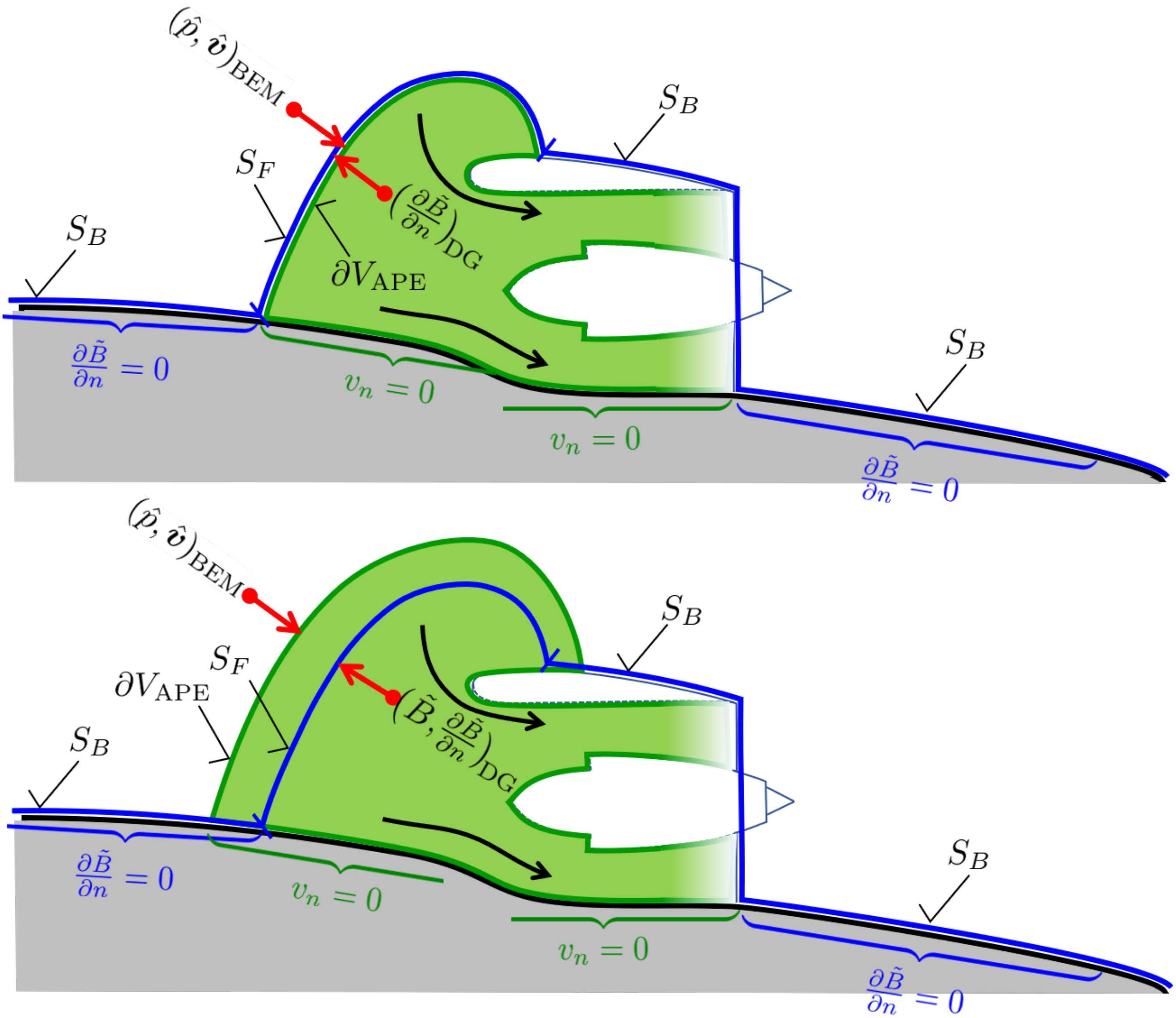
Now, the coupling of the acoustic surface integral (10) to the 3D APE domain may be done in two different ways as sketched in Figure 2. The strong coupling is realized in an iteration process. The exchange of data takes place after a couple of pseudo time steps of the Runge Kutta scheme (the exact number of RK steps before data exchange appeared not to have an effect on the final solution):

1. In the first approach, the surface S _F is identical with a part of the free boundary ∂V_APE of the 3D APE domain from where $\raisebox{1ex}{$\partial B˜$}\!\left/ \!\raisebox{-1ex}{$\partial n$}\right.$ is specified. The surface elements on S _F are arranged to fit onto the volume cell faces forming ∂V_APE in order to allow for a cell face wise 2D interpolation of data. The boundary values from the APE are subject to the local NRBCs based on Riemann invariants and so they represent an approximation only. The communication between S _F and APE is accomplished by use of (8), (3) and (4):

*3D APE domain → Integral surface S _F :

One obtains $\raisebox{1ex}{$\partial B˜$}\!\left/ \!\raisebox{-1ex}{$\partial n$}\right.=-i\omega T\mathit{n}\cdot \left(\widehat{\mathit{v}}+\frac{\widehat{p}}{{\rho }^0{a}_0^2}{\mathit{v}}^0\right)$ to first order in M. Then the integral equation (10) is solved for $\tilde{B}$ on S. Since (10) satisfies the radiation condition exactly (even in the near field), feeding back $\tilde{B}$ onto the free boundary of the APE domain not only contains the acoustic influence of the walls of the aerodynamic body S _B , but also corrects for the approximate NRBCs.

* Integral surface S _F → 3D APE domain:

The respective variables derived from $\tilde{B}$ on ∂V_APE are $\widehat{p}={\rho }^0\left[\tilde{B}+{\mathit{v}}^0\cdot \mathit{\nabla }\tilde{B}/\left(i\omega \right)\right]T^{-1}$ and $\widehat{\mathit{v}}=-\left[\mathit{\nabla }\tilde{B}/\left(i\omega \right)+\tilde{B}{\mathit{v}}^0/a_0^2\right]T^{-1}$ .

A new APE solution is now generated with these boundary values on ∂V_APE starting the next step in the iteration until convergence is reached.

2. In the second approach the 3D APE domain extends somewhat beyond S _F , so that there exists a layer of a few grid cells between S _F and ∂V_APE. In contrast to the first approach the complete integrand on S _F is specified by volumetric interpolation from within the APE domain V_APE. First, the integral equation (10) is now solved for $\tilde{B}$ on S _B using α = 1/2. Then the solution is evaluated for x on ∂V_APE with α = 1. Since this data is evaluated on the basis of (10), again the radiation condition is satisfied along with communication of the acoustic presence of S _B .

* 3D APE domain → Integral surface S _F :

$\tilde{B}=T\left(\widehat{p}/{\rho }^0+{\mathit{v}}^0\cdot \widehat{\mathit{v}}\right)$ and $\raisebox{1ex}{$\partial B˜$}\!\left/ \!\raisebox{-1ex}{$\partial n$}\right.=-i\omega T\mathit{n}\cdot \left(\widehat{\mathit{v}}+\frac{\widehat{p}}{{\rho }^0{a}_0^2}{\mathit{v}}^0\right)$ is obtained from volumetric interpolation (evaluation of ansatz-polynomials inside DG method) from the APE domain V_APE onto S _F . Then the integral equation (10) is solved for $\tilde{B}$ on S _B . Since (10) satisfies the radiation condition exactly (even in the near field), evaluating $\tilde{B}$ and $\raisebox{1ex}{$\partial B˜$}\!\left/ \!\raisebox{-1ex}{$\partial n$}\right.$ onto the free boundary of the APE domain not only contains the acoustic influence of the walls of the aerodynamic body S _B , but also corrects for the approximate NRBCs.

* Integral surface S _F → 3D APE domain:

The respective variables derived from $\tilde{B}$ and its gradient on ∂V_APE are $\widehat{p}={\rho }^0\left[\tilde{B}+{\mathit{v}}^0\cdot \mathit{\nabla }\tilde{B}/\left(i\omega \right)\right]T^{-1}$ and $\widehat{\mathit{v}}=-\left[\mathit{\nabla }\tilde{B}/\left(i\omega \right)+\tilde{B}{\mathit{v}}^0/a_0^2\right]T^{-1}$ .

A new APE solution is now generated with these boundary values on ∂V_APE starting the next step in the iteration until convergence is reached.

Figure 2.

Coupling of surface integral (blue) and APE domain (green). Top: coupling approach 1, bottom: coupling approach 2.

Remark 1

It was observed that particularly approach 2 leads to a stable and fast convergence to the final solution. Note, that in comparison to approach 1 the solution of the boundary integral equation (10) is reduced to $\tilde{B}$ on S _B for approach 2. This comes at the expense of an additional evaluation of $\tilde{B}$ on S _F . Another advantage over approach 1 is that the Burton Miller procedure is not needed on the S _F part of the surface, because the complete APE data on this part of S avoids artificial resonance for eigenfunctions as part of this boundary. Moreover, as opposed to approach 1 the data generated on S _F by (10) and feeding back onto ∂V_APE is evaluated from non-singular integrals. An additional plus for approach 2 is the volumetric interpolation of data which practically allows for non-matching surface grids at the interface to S _F . Finally, the a gap between the free APE boundary and the coupling surface is beneficial to reduce approximations in the fast multipole method. Because of these advantages all simulations shown in this paper were carried out on the basis of approach 2.

Remark 2

In applications where not much scattering of sound from S _B is present, a loose coupling, i.e. doing only one solution of (10) may be sufficient. Then feeding back the solution into a new APE solution step may be avoided. If S _B is neglected altogether, the solution may be evaluated explicitly at any point in the field (as a typical FW-H simulation would do).

Applications

This section is devoted to demonstrating the use of the presented efficient simulation approach for the sound radiation in the presence of flow and scattering objects. In a first example the capability of the strong coupling between DG and FM-BEM is shown to provide very accurate NRBCs for very small DG domains, even when the free boundaries are located in the nearfield of sources. This feature to provide very clean acoustic boundary conditions is important in itself, because small DG local domains do naturally occur in the applications, where large aircraft surfaces are to be taken into account in order to include acoustic scattering. Further examples demonstrate the computation of the sound radiation from fully aircraft installed engine intakes, emphasizing the importance of taking into account the local nonuniformity of the flow near the intake.

Radiation from source distribution in free space

This problem is designed to test the strong coupling approach 2 for its ability to realize practically perfect NRBCs at artificial domain boundaries. The example is deliberately chosen as a very simple case of a Gaussian heat source $\widehat{\vartheta }=\exp \left(-\text{ln}2\raisebox{1ex}{${\left|\mathit{x}\right|}^2$}\!\left/ \!\raisebox{-1ex}{$b^2$}\right.\right)$ in free space and quiescent medium, centered at the origin with a Gaussian half width of b = 0.1 m and a wavelength of λ = 1m. The upper left part of Figure 3 depicts the computational domain chosen. The domain V_APE consists of a sphere of radius R_APE = 1.2 m, centered on the origin cropped by a plane at z = 0.4 m. The BEM surface is concentric with $R_{S_F}=1.0\text{m}$ . The blue part shows the surface S _F , which (since no foreign body surfaces S _B are present) is entirely embedded into the green volume V_APE. One may observe that the cell size on S _F is chosen smaller by about a factor of 1/3 than in V_APE, because the DG APE solver DISCO++ is of fourth order, while the BEM solver FMCAS is only first order. The discretization is chosen as to ensure good resolution, since numerical resolution studies are not intended in this paper. The 3D APE domain contains 7336 tetrahedra while 9938 triangles were used for the surface integral; both discretizations are equivalent to roughly 20PPW.

Figure 3.

Test of coupling concept on generic case: zero flow, point heat source at x, y, z = 0, 0, 0, realized as Gaussian distribution with half width b = 0.1 m. Lower row: a) coupled with cropped spherical domain, b) uncoupled with cropped spherical domain (DG solution only), c) uncoupled with spherical domain (DG solution only), d) coupled with spherical domain (“reference”), upper row: left: blue: FMCAS surface, green: domain boundary for DG, centre and right: error w.r.t. case d) on intersections along green lines from bottom contour plots; orange dashed line: location/extension of Gaussian source.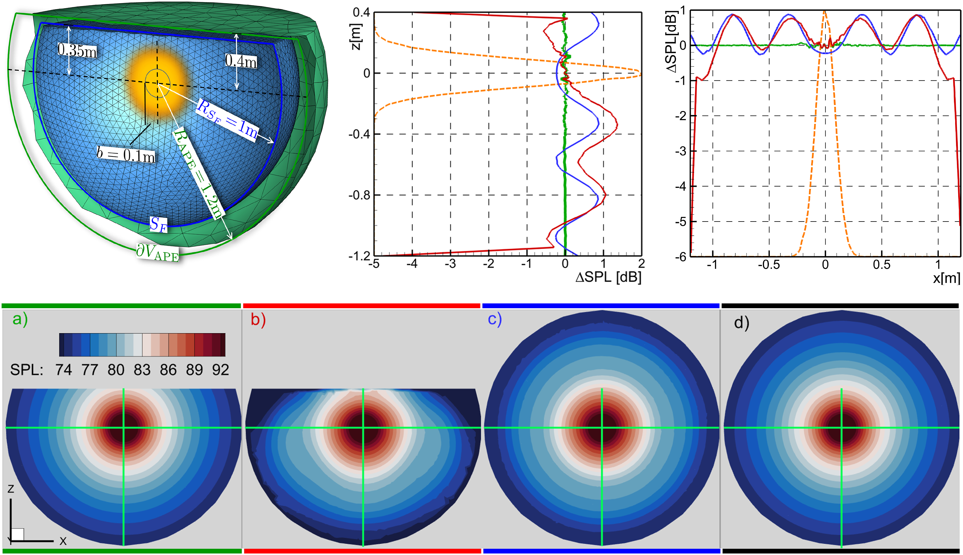

The lower row of Figure 3 depicts the results of the numerical solution to this problem in terms of the contour lines of the sound pressure level in V_APE. Despite the cropped (nonsymmetric) domain to the symmetric problem the left figure shows perfectly concentric contour lines, case (a). Note that the boundaries are in the nearfield of the source because (i) the source is extended and (ii) the particle velocity (even of a point mass source!) would contain a nonradiating 1/r² component. The second challenge to the NRBCs here is that the sound wave hits the flat part of the boundary at a shallow angle. The shown solution is obtained after very few iterations between the DG solution and the surface integral. In contrast to case (a) the second left contour plot in the lower row of Figure 3 (case (b)) displays strong distortions of the contour lines, particularly near the nonsymmetric (flat) part ot the domain boundary. This outcome would result in a typical standalone DG APE solver, with charactistics based NRBCs, where incoming fluxes are set equal to zero (no coupling to BEM). In other words, (b) shows the result of the initial step in the iteration process, which upon continuation would yield the result in (a).

In order to gain more insight into the results obtained, the second plot to the lower right depicts another test, denoted case (c), featuring the same characteristics-based NRBCs as in case (b), but avoiding any waves with shallow incidence on the boundaries as now S _F represents a spherical surface and V_APE a spherical volume, both concentric with the source. As expected, now the contour lines of the SPL are perfect spheres; the distortions seen in (b) do not appear. However, a detailed look at the contour lines in case (c) compared to case (a)) reveals that their spacing is somewhat different. It is therefore worthwhile comparing the solutions to yet another case (d), shown in Figure 3 on the lower right. Here, the coupling to the BEM is employed as in case (a). The SPL contour lines of this best approximation to the solution are in practically perfect agreement with case (a). The question arises, why there remains a difference in the contour lines in cases (c) and (d) even for this choice of domain with all waves exiting normal to the boundaries and thus providing for a seemingly best applicability of the local, characteristics based NRBCs. The reason becomes apparent by inspecting the characteristics based boundary conditions, used in case (c), which sets the incoming flux equal to zero, irrespective of whether the true signal still contains non-propagational (near field) components. While this condition is appropriate in the far field, where the non-propagational components have decayed sufficiently, this is not the case for the considered test example. The domain was deliberately chosen to represent an applied problem, in which the APE domain would be as small as possible in order to save computational resources. For this reason setting the incoming flux equal to zero is incorrect. It leads to conversion of the near field components into sound propagating back into the domain. Finally, it is worthwile considering the errors by evaluating the difference in SPL with respect to case (d), i.e. ΔSPL = SPL − SPL _d . This is displayed in the contour plots of Figure 3 along a vertical and a horizonal line section as indicated in green. The diagrams in the top right of the figure show the various ΔSPLs, in which the position and extent of the Gaussian source is indicated in orange. Clearly, the coupled solution (a) in the cropped domain is in perfect agreement with the reference case (d) everywhere. Cases (b) and (c) instead show noticeable deviations. The uncoupled simulation in the cropped domain, case (b), obviously yields errors of up to 6 dB near the boundaries. The error in the interior is very similar to the one observed in the simulation result of case (c) with a symmetric domain and amounts to about 1 dB. This error in the interior displays an oscillatory shape which corresponds to a standing wave pattern of a wave with the specified wavelength of unity. As a conclusion the example shows that the strong coupling of the fast multipole solver FMCAS for the acoustic surface integral (10) with the DG solver DISCO++ for the APE indeed yields a clean solution with practically perfect radiation conditions even if the boundaries are located inside the near field.

Fan radiation from integrated turbofan intake

The fan forward sound radiation from a semi-buried engine intake integrated at the aircraft’s fuselage is considered at low speed conditions (take-off, landing), see Figure 4. Such kind of configurations are of interest because the ingestion of the fuselage’s boundary layer may improve the overall propulsion efficiency particularly at cruise conditions. From an aeroacoustics point of view there are two aspects of such kind of arrangement, (a) the ingested boundary layer potentially increases the sound generation at the fan due to unsteady blade loads, (b) the sound propagation through the duct and further on to the (non-circular) intake where strong local flow gradients are present, and finally the sound radiation under the influence of the aircraft surface. Assuming a suitable fan sound generation model (e.g. Moreau ²⁰ provides the sound field, the complex radiation, i.e. aspect (b) needs to be computed, which will be addressed in this example application of the BEM-DG coupling. The volume-resolving simulation of the APE is needed in the intake where high flow speeds are present and in the immediate vicinity of the intake since strong flow gradients need to be accounted for. Already near the intake the outer flow may be considered a slender body potential flow at Mach numbers on the order of the (low speed) flight Mach number, where the gradients are moderate. Therefore the use of the surface integral (10) is justified to acoustically account for all the rest of the aircraft’s surface.

Figure 4.

left: Aircraft configuration with rear fuselage engine and an intake, buried into the fuselage by about 15% of the fan diameter; right: choice of integration surfaces S _B , S _F and free boundary of APE domain for coupling approach 2.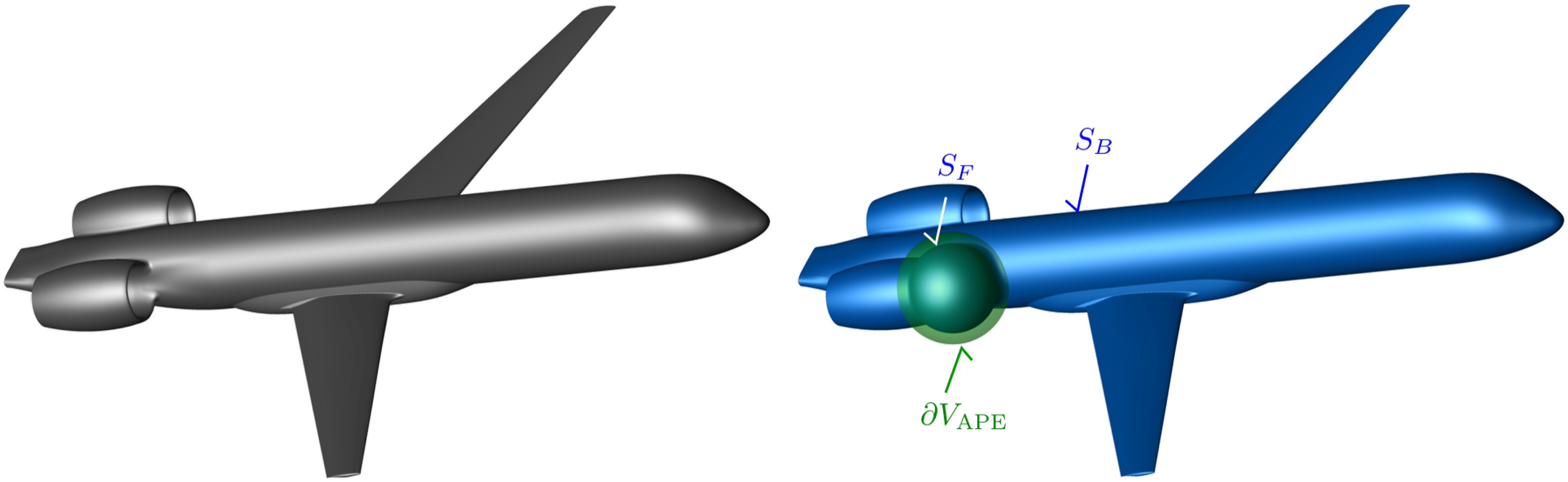

A DLR research aircraft configuration with forward swept wings with a span of 34m is considered which features semi-buried engine intakes at its rear fuselage. In the design variant depicted in Figure 4 the buring depth is equal to 15% of the fan diameter. The aircraft is in take-off conditions and flies at a Mach number of M _F = 0.25. Fan sound generation is considered at at frequency of f = 582.7 Hz at full scale, the fan modes are specified by DLR’s inhouse analytical method PropNoise. ²⁰

The introduced coupled BEM/DG computation concept is used to investigate the significance of the intake mean flow inhomogeneity on the overall sound radiation of the aircraft. Approach 2 of the coupling is adopted (see previous section); therefore the APE domain V_APE somewhat extends beyond the BEM surface S _F as seen in the right of Figure 4. The local flow near the intake, determined by numerical solution of the RANS equations with DLR’s inhouse CFD code TAU is characterized in the top part of Figure 5. The two sections through the intake show strong acceleration. Due to the blending with part of the the nacelle and the fuselage the flow is highly non-axisymmetric. One may also see that the boundary layers are quite thin, so the flow field features almost completely potential flow. In the centre part the free surface of the APE domain ∂V_APE is displayed along with the isolines of the flow speed. The surface was chosen such that the flow is almost uniform as indicated by the isolines. The right picture, showing the speed distribution from another view, underlines this feature. Note, that the flight speed of the aircraft corresponds to a value of | v ⁰|/a _∞ = 0.25. For this reason, the potential of the mean flow, used in Taylor’s transform was approximated by ϕ⁰ = M _F a _∞ x.

Figure 5.

Local flow and sound pressure near 15% buried intake; upper row shows the flow field simulated on the basis of the RANS, the green surface depicts the free boundary of the APE domain; speed values as isolines indicate almost uniform flow. Lower row depicts the APE solution; left: snapshot (real part) of sound pressure p^ constant flow assumption everywhere, right: same, but with actual background flow.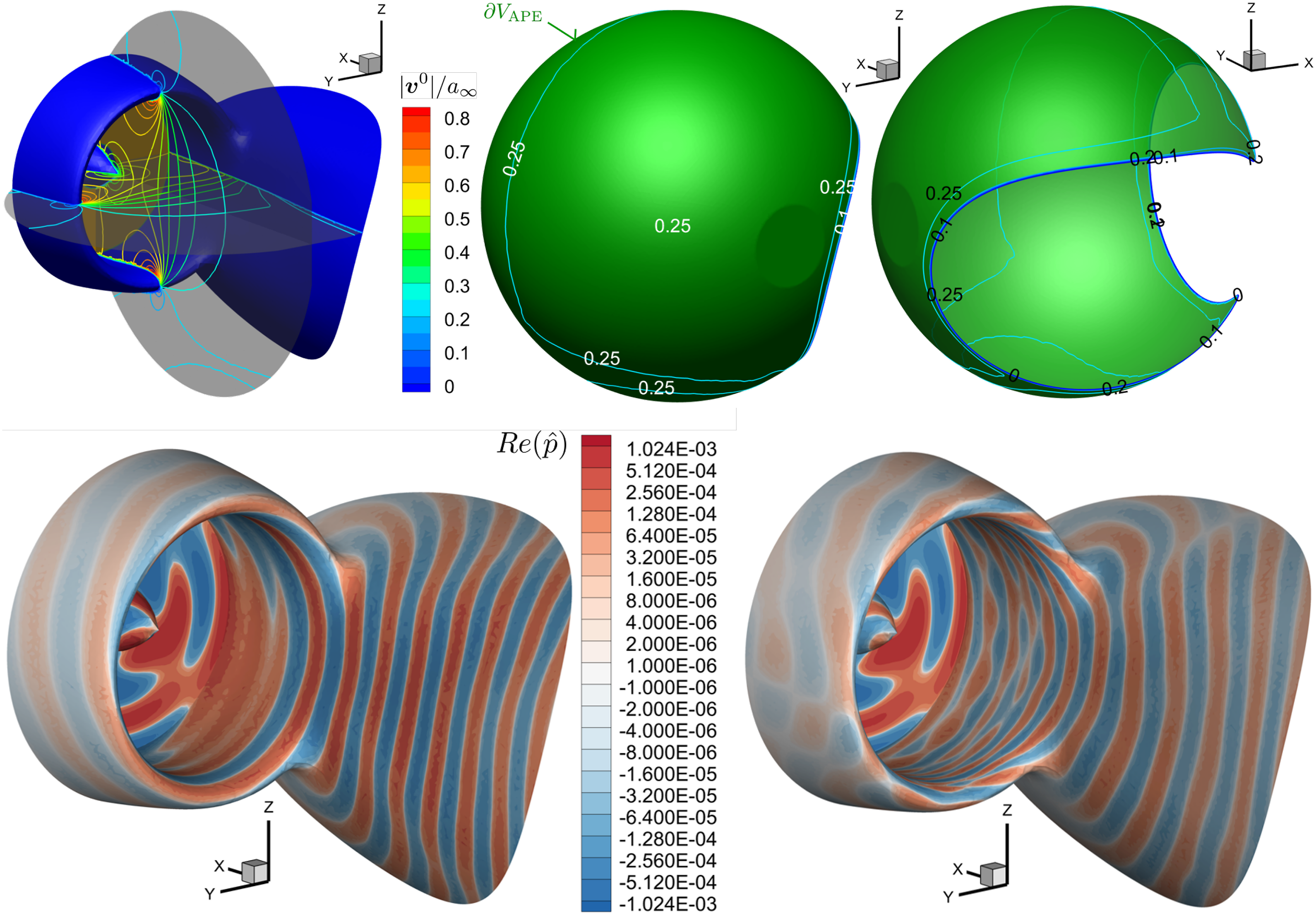

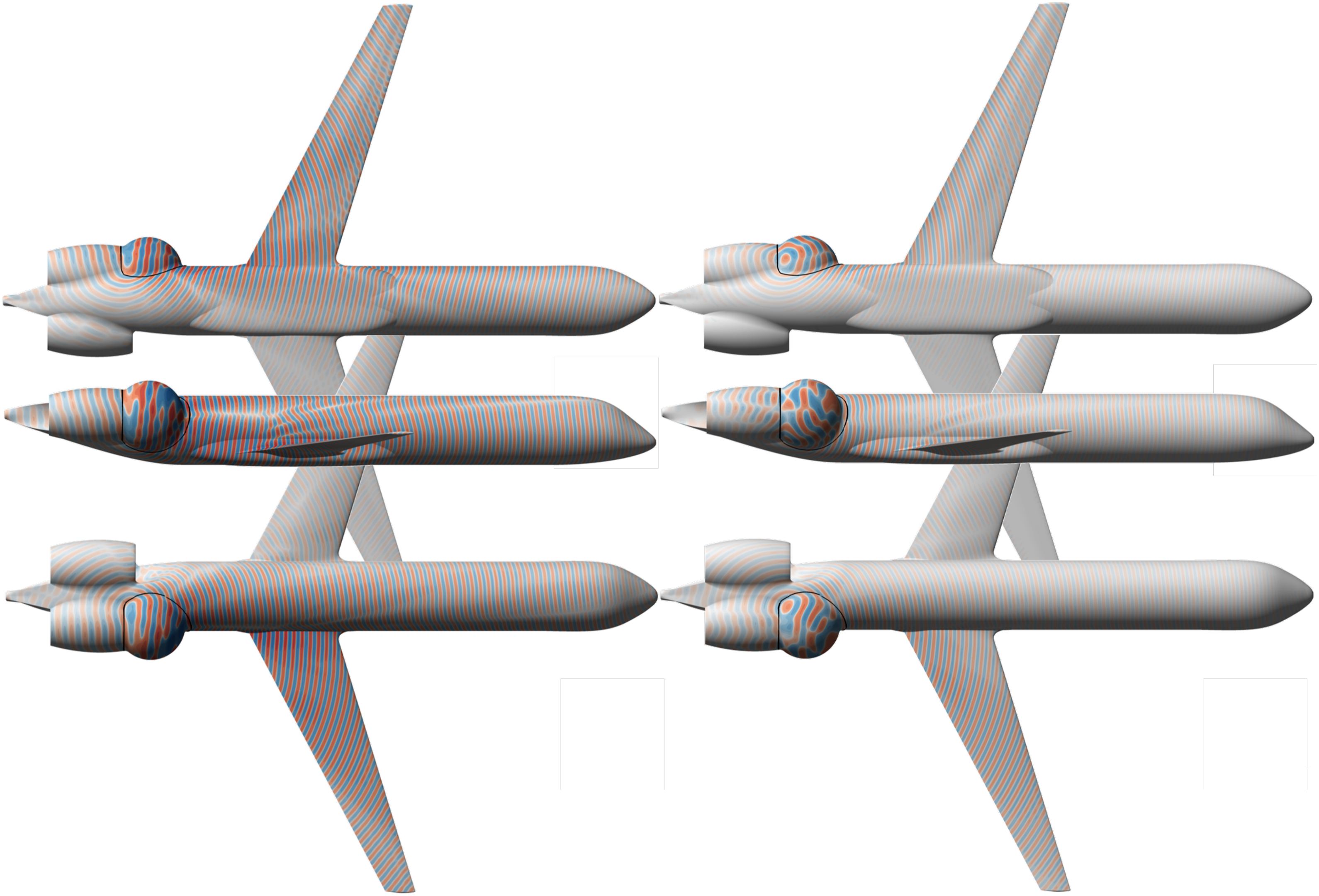
Figure 5 depicts the sound pressure field distribution near the intake. The left part of the figure shows the result for uniform flow (flight speed throughout), while the right part displays the pressure using the actual flow field. The influence of local flow inhomogeneity on the sound radiation is apparent; large differences may be observed particularly in the wave diffraction around the lip of the nacelle. The pressure signature at this position and inside the duct suggests that the presence of the inhomogeneous flow enhances the scattering of the fan modes into more complex (“higher order mode”) structures. This effect is even more accentuated when the intake is buried deeper into the fuselage as may be observed in figure 6. The modification of the pressure signature due to the non-uniform flow may again be observed on the snapshot of the distribution of $\widehat{B}$ on the complete aircraft surface in figure 7.

Figure 6.

Local flow and sound pressure near 55% buried intake; upper row shows the flow field simulated on the basis of the RANS, the green surface depicts the free boundary of the APE domain; speed values as isolines indicate almost uniform flow. Lower row depicts the APE solution; left: snapshot (real part) of sound pressure p^ constant flow assumption everywhere, right: same, but with actual background flow.

Figure 7.

Snapshot of surface values of B^ for aircraft with 55% buried intake in various views; left: uniform flow assumption, right: RANS flow.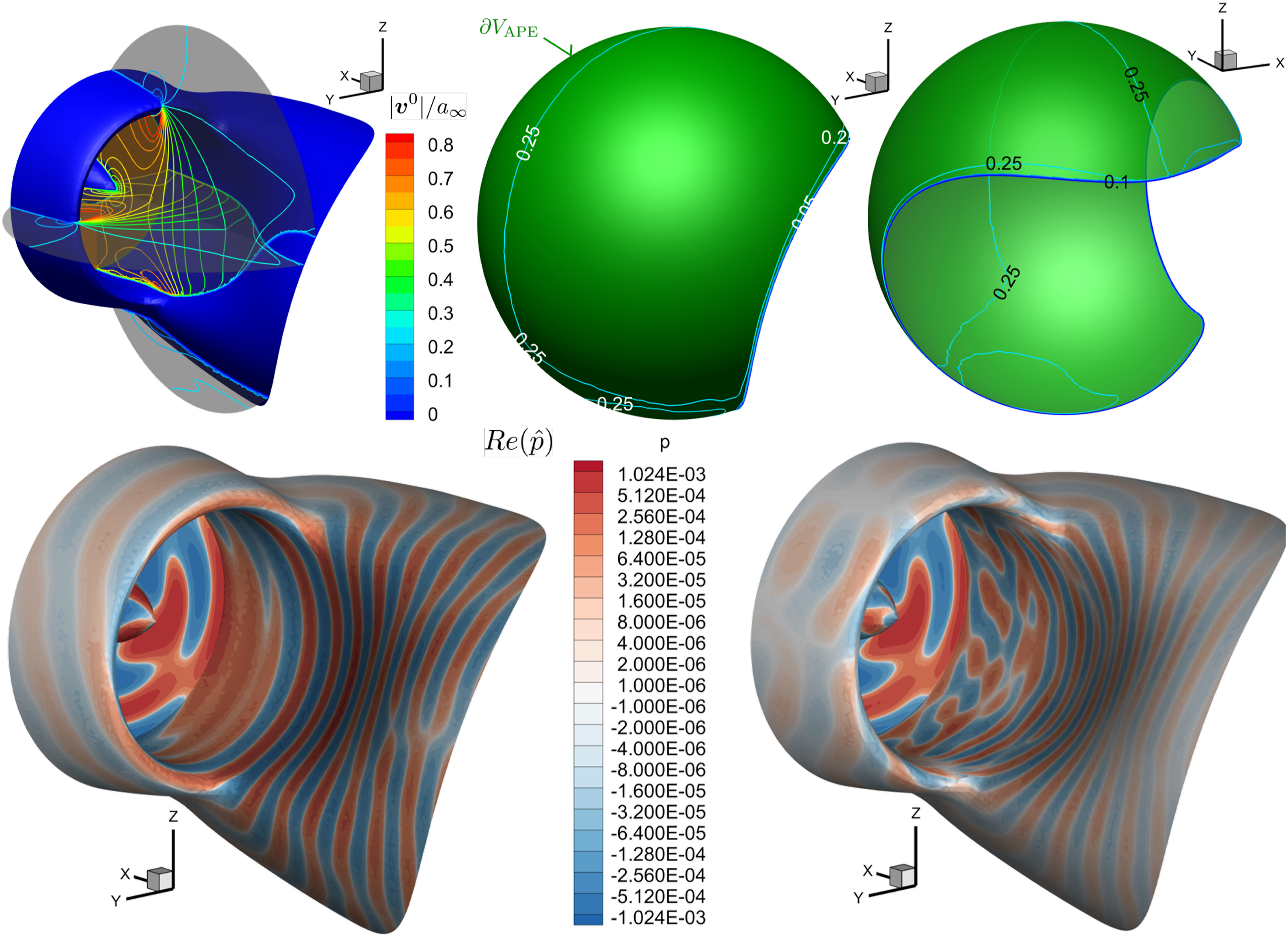

The far field radiation is analysed by using the wave extrapolation function of the FM-BEM code (choosing α = 1 in equation (10)). Observers in a plane 50m below the center of the fan are choosen. The footprint of only one (the starboard) engine is considered because this gives a clearer view on the shielding. The fan source noise is kept constant (specified fan modes in the fan plane) for all considered variations in order to isolate the net installation effect on the radiation. Results are shown in figure 8. Clearly, the noise contours turn out very different depending on the flow field used. The assumption of uniform mean flow leads to a much more extended footprint and to higher levels too. This is true for both integrations of the engine (15% and 55%), the difference being even larger for the aircraft with the 55% integration. For the 15% buried nacelle case the maximum contour level turns out to be 3 dB too high if uniform mean flow is assumed, whereas this error amounts to about 18 dB! for the 55% buried nacelle. Moreover, it is observed that the footprint computed with uniform mean flow looks qualitatively similar for both integration configurations, while this is not the case if the realistic mean flow is used. In order to convey an impression of the computation time it is noted that one complete simulation typically took a total of 450 min of wall clock time on 4 nodes* for the DG APE solver (150 min = 140 min in solver loop + 10 min communication) and 1 node for the BEM solver (300 min = 107 min in solver loop + 193min mostly i/o).

Figure 8.

Evaluation of sound pressure contours 50m below the aircraft. Upper row, left: result for assumption of uniform mean flow, right: the same for realistic mean flow for a/c with 15% burying level. Lower row: same as above, but for 55% burying level of nacelle, grey colorscale corresponds to level of B on a/c surface.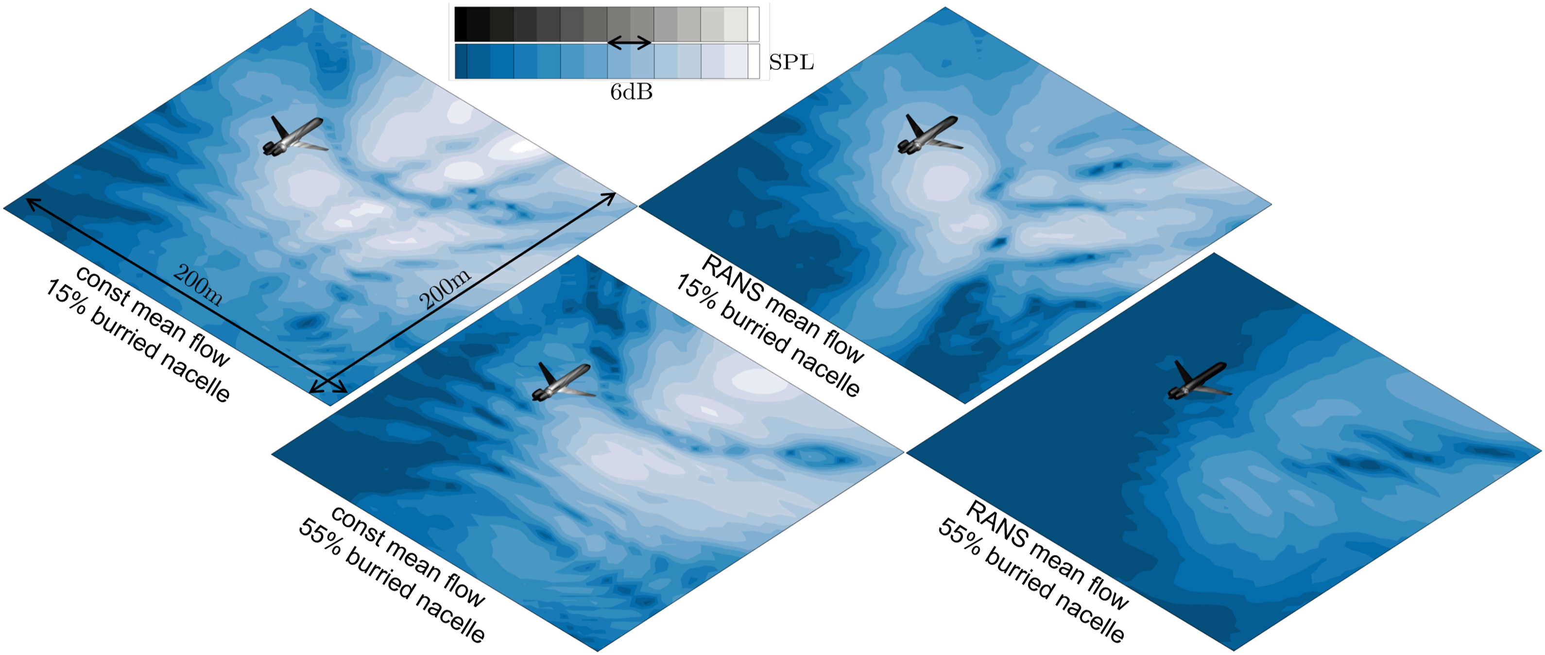

Finally, a comparison between the two integration configurations based on the results obtained with realistic mean flow reveals a much stronger (positive) shielding effect for the 55% buried nacelle, compared to the 15% case. Clearly, the fuselage shields much of the fan sound otherwise radiated to the portside direction. This study shows that in order to predict the radiation of sound from an installed fan it is very important to take the true flow situation into account even only for the radiation part of the problem. In a next step it is interesting to study the modification of the fan source in response to non-uniform inflow, e.g. Wisda ²¹ ; Murray ²² and in combination with the modified propagation situation as e.g. studied in Romani. ²³ The question to be answered is, whether any excess source noise at the fan counterbalances the observed benefits of the shielding.

Summary and Conclusions

A coupled computation approach is presented which combines a volume resolving Discontinuous Galerkin code (DISCO++, DLR) with a Fast Multipole Multi Domain BEM code (FMCAS, DLR). The DG code solves the APE equation while the FM-BEM code solves Möhring-Howe’s wave equation, Taylor-transformed to the Helmholtz equation. The exact description of propagation effects in the domain outside the APE domain is therefore restricted to low Mach numbers (and small gradients of it). Such conditions are however quite realistic for aircraft at low speed, where noise issues matter. The combined method realizes a two way coupling, based on iteratively exchanging data on a common interface at each pseudo time step of the frequency domain DG code. The procedure is implemented in the frequency domain in order to take full advantage of the fast multipole acceleration techniques. A coupling concept (called approach 2) based on a slight overlap of the DG domain over the free surface of the BEM is found to work robustly.

It is found that the strong coupling enables very small DG domains with practically perfect non reflecting boundary conditions. An example of tonal fan sound radiation of a turbofan engine, tightly integrated into the rear fuselage of an aircraft is investigated. The proposed computation approach proves capable of taking into account non-trivial flow effects near the installed intake revealing a strong influence on the far field radiation, depending on the configuration.

The presented computation approach provides fast turnaround times while taking into account important flow effects on the sound radiation, which cannot be neglected. It is therefore suitable for design studies, in which the source is modelled, e.g. with semi-analytical tools as DLR PropNoise ²⁰ or numerical models of (installed) rotors based on body forces^{6, 7} and it may also provide a means to restrict expensive simulations of sources to smaller computation domains.