Sage Journals: Discover world-class research

Abstract

Trailing-edge noise is known to be sensitive to airfoil shapes, and ice accretion is one cause of an airfoil shape deformation. This paper investigates how trailing-edge noise is affected by the airfoil shape deformation due to ice accretion. The formation of ice-induced flow separation and the development of a turbulent boundary layer are analyzed to understand the correlation between the altered flow physics due to ice accretion inside the boundary layer and trailing-edge noise. The near-wall flow behind the leading-edge ice accretion is analyzed by using Reynolds-Averaged Navier Stokes CFD in OpenFOAM, and trailing-edge noise is investigated using an empirical wall pressure spectrum model in conjunction with Amiet’s trailing-edge noise theory. Validations of tools against measurement data are presented. Liquid water content, freestream velocity, and ambient temperature are varied to investigate the impact of flow conditions on the ice accretion shape and the resulting boundary layer flow characteristics at the trailing edge. It is found that a more significant leading edge deformation due to ice accretion generates larger ice-induced flow separation bubbles, which increases the trailing-edge boundary layer thickness. As a result, an increase in low- and mid-frequency noise is observed. The purpose of this paper is not only to understand the effect of ice accretion on trailing-edge noise but also to comprehensively analyze how flow physics inside the turbulent boundary layer is altered by the presence of various ice accretion shapes.

Keywords

Ice accretion turbulent boundary layer trailing-edge noise CFD Reynolds-Averaged Navier Stokes

Introduction

Turbulent boundary layer trailing-edge noise is characterized as a dominant noise source among the sources of airfoil self-noise.¹ The eddies developed within the turbulent boundary layer near the trailing edge generate unsteady surface pressure fluctuations, and the scattering of this wall-bounded pressure fluctuations by a sharp trailing edge induces trailing-edge noise.² This noise is notably important for wind turbine³ and rotorcraft^4–6 applications as well as aircraft during landing. Trailing-edge noise is sensitive to airfoil shape and size,^7,8 in addition to flow conditions. Understanding how these factors contribute to trailing-edge noise is crucial to eventually achieving lower overall noise levels.

Ice accretion is a serious problem in aircraft since it degrades overall performance, which is directly related to passengers’ safety or mission failure. Many studies have already shown the degradation of aircraft performance due to ice accretion. Kelly et al.⁹ presented helicopter rotor performance degradation through 2D and 3D hybrid simulations. Moreover, concerns with the ice accretion during an operation of eVTOL vehicles have also been growing with the rise of the eVTOL industry. McKillip et al.¹⁰ presented that the ice accretion is more likely to develop at a lower altitude, at which eVTOL vehicles are expected to operate. Scroger et al.¹¹ experimentally demonstrated thrust degradation of an urban air mobility (UAM) rotor. Ice accretion is also developed on wind turbine blades in cold weather. The ice accretion on wind turbine blades results in the reduction in the wind power generation.¹² While myriads of studies have shown that accumulated ice at the leading edge affects the aerodynamic performance, not enough studies have been conducted to investigate the effect of ice accretion on trailing-edge noise. Since the trailing-edge noise is sensitive to airfoil shape, it is hypothesized that the ice accretion at the leading edge would impact the trailing-edge noise generation. The ice accretion at the leading edge during aircraft or wind turbine operation in cold weather could significantly alter boundary layer flows over the entire airfoil section and the resulting trailing-edge noise.

Understanding the shapes of accreted ice provides insights not only on aerodynamic behaviors but also on noise generation. Various ice shapes are formed on the leading edge of an airfoil under different flow conditions. Rime icing is developed when the ambient temperature is extremely low such that water droplets freeze at an instant moment of contact with the airfoil surface. On the other hand, a glaze icing is developed at a relatively warmer temperature than the rime icing condition such that water droplets smear on the airfoil surface before freezing. In a paper by Son et al.,¹³ liquid water content (LWC) is shown to contribute to ice shapes in glaze icing conditions, while the freestream velocity and ambient temperature define ice shapes in both glaze and rime icing conditions. Morelli et al.¹⁴ studied flow and acoustic characteristics of glaze and rime ice for an oscillating airfoil. They showed that the ice accretion on the leading edge significantly alters noise characteristics. In their study, however, unsteady Reynolds-Averaged Navier Stokes (RANS) CFD was used to capture pressure fluctuations on the surface that were induced by the ice accretion. Hence, their study does not reveal boundary layer turbulent trailing-edge noise on an iced airfoil. Cheng et al.¹⁵ showed that the ice-induced roughness during the early stage of ice accretion on an airfoil surface increases broadband noise while emphasizing that the ice-induced roughness is negligible for longer icing time or the icing condition exposure time. Our research focuses on the trailing-edge noise as a result of fully developed ice accretion for a long exposure time; therefore, the ice-induced surface roughness is not considered in the current paper.

The shape change of the leading edge of the airfoil due to ice accretion will produce unsteady flow characteristics. Although the unsteadiness of the flow may generate other sources of noise, the paper focuses on the noise generated by the scattering of the wall-bounded pressure fluctuations by the trailing edge. Since the ice accretion at the leading edge generates turbulence downstream, the laminar boundary layer vortex shedding noise does not contribute to the total noise. Although it is found that the flow separates behind the ice horn, it reattaches before it reaches the trailing edge and the separation does not cause stall for the given angles of attack. Therefore, the stall noise is neglected. The problem considered in this paper is two dimensional, so the tip vortex formation noise is disregarded as well. The airfoil trailing edge is blunt, so the bluntness noise may contribute to the total noise, but according to Brooks et al. Ref.1, the turbulent boundary layer trailing-edge noise is far more dominant compared to the bluntness noise in a wide range of frequency.

In this paper, the effect of ice accretion on the trailing-edge boundary layer parameters as well as the resulting trailing-edge noise is investigated using RANS CFD and Amiet’s trailing-edge noise model in conjunction with an empirical wall pressure spectrum model. The primary purpose of this paper is to analyze how a formation of ice-induced flow separations at the leading edge affects boundary layer flows at the trailing edge and thus trailing-edge noise at different operating conditions. We will first present the detailed validations of ice accretion shapes, boundary layer flows under a representative icing condition, and trailing-edge noise predictions. Next, detailed analyses of boundary layer flow physics for various ambient conditions will be presented to reveal correlations between the ice shapes and boundary layer parameters.

Method

Figure 1 shows a step-by-step process of predicting trailing-edge noise from given icing and flow conditions. The ice accretion is first predicted by NASA’s analytical ice accretion model, LEWICE¹⁶ program. LEWICE evaluates the freezing process thermodynamics that occur when super-cooled droplets impinge on a body. Both atmospheric parameters (i.e. temperature, pressure, and velocity) and meteorological parameters (i.e. liquid water content, droplet diameter, and relative humidity) are used to determine the shape of the ice accretion. Open source tools, Gmsh¹⁷ and OpenFOAM,¹⁸ are used to generate airfoil meshes and run RANS CFD, respectively. From the CFD results, boundary layer input parameters for Lee’s wall pressure spectrum model¹⁹ are obtained, from which the trailing-edge noise is predicted using the Amiet theory.

Figure 1.

Step-by-step noise analysis process.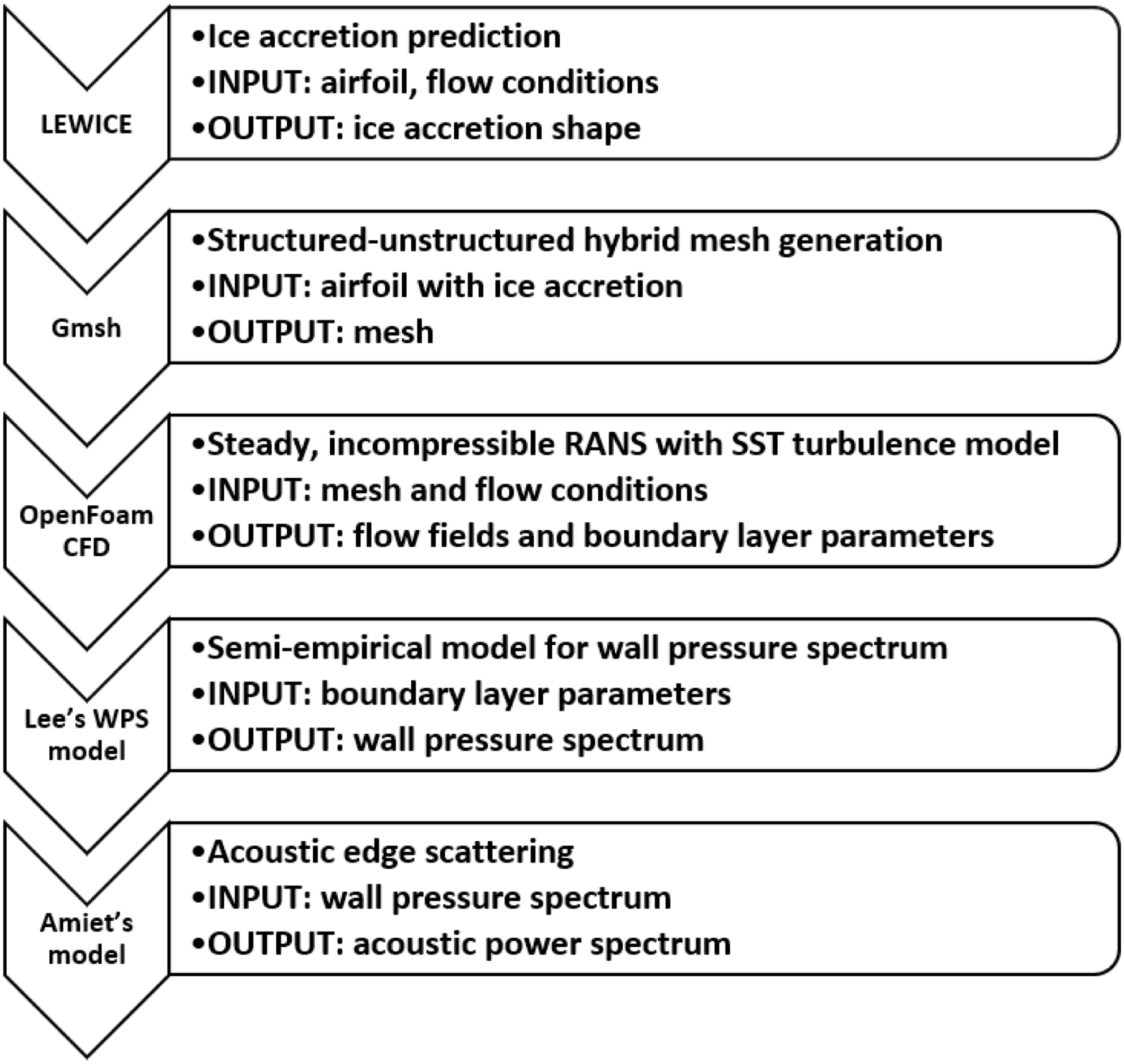

Mesh generation

Since numerous ice shape cases are considered in this paper, a quick and effective way of mesh generation is necessary. Gmsh is designed to easily produce an unstructured mesh for a CFD analysis. By introducing a structured-unstructured hybrid mesh (structured near the airfoil surfaces and unstructured in far field), CFD results can be obtained at a faster pace but still be accurate enough near the airfoil surfaces to accurately capture boundary layer profiles. As an example, a mesh of one of the iced airfoils studied in this paper (case 2e) is shown in Figure 2. Approximately 50–100 mesh nodes are placed on the ice accretion depending on the ice shapes, and approximately 150 nodes are placed on each suction and pressure side of the airfoil. Y⁺ of at or less than one along the surface of the airfoil is maintained.

Figure 2.

Hybrid mesh of one iced airfoil: (a) entire airfoil volume mesh and (b) enlarged view near the leading edge.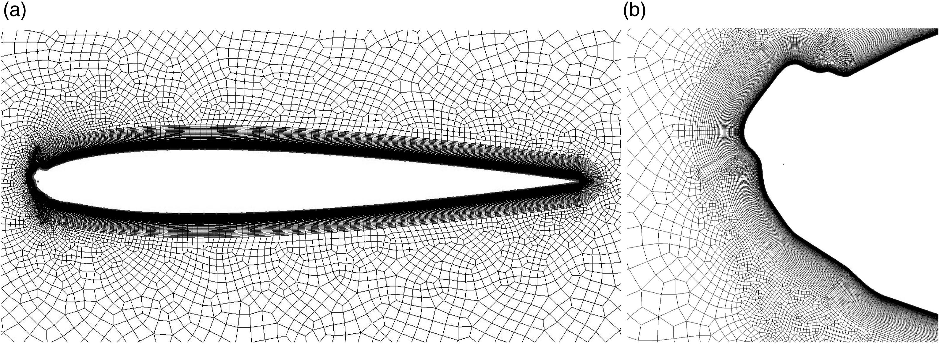

Computational fluid dynamics

CFD is executed using a K-Omega SST turbulence model in OpenFOAM to analyze aerodynamic performance, flow field, and boundary layer parameters near the trailing edge. CFD results are post-processed through Paraview, from which the pressure and friction coefficients around the airfoils as well as the velocity and TKE profiles at 99% of the airfoil chord from the leading edge are obtained. With this information, six boundary layer input parameters are determined: edge velocity (U_e), boundary layer thickness (δ), displacement thickness (δ*), momentum thickness (θ), friction coefficient at 0.99c (C_f), and pressure gradient along the streamwise or x direction at 0.99c (dP/dx). The boundary layer thickness is determined based on the TKE profiles, a method similar to that developed by Catlett et al²⁰. Unlike Catlett et al.’s method, which uses $T K E (δ) = 0.0002 U_{0}^{2}$ , this paper determines the boundary layer thickness by finding a location where the turbulent kinetic energy approaches zero above the peak value: ΔTKE < 10⁻². Figure 3 shows the normalized TKE and velocity profiles of case 1a studied in this paper (shown in the Result section) to visually represent the method of the boundary layer thickness prediction using a TKE profile. The horizontal dashed line indicates the boundary layer thickness, which is determined from the TKE criterion as discussed above. The vertical dashed line indicates the normalized velocity magnitude at the boundary layer thickness or the normalized boundary layer edge velocity.

Figure 3.

Boundary layer thickness prediction using a TKE profile.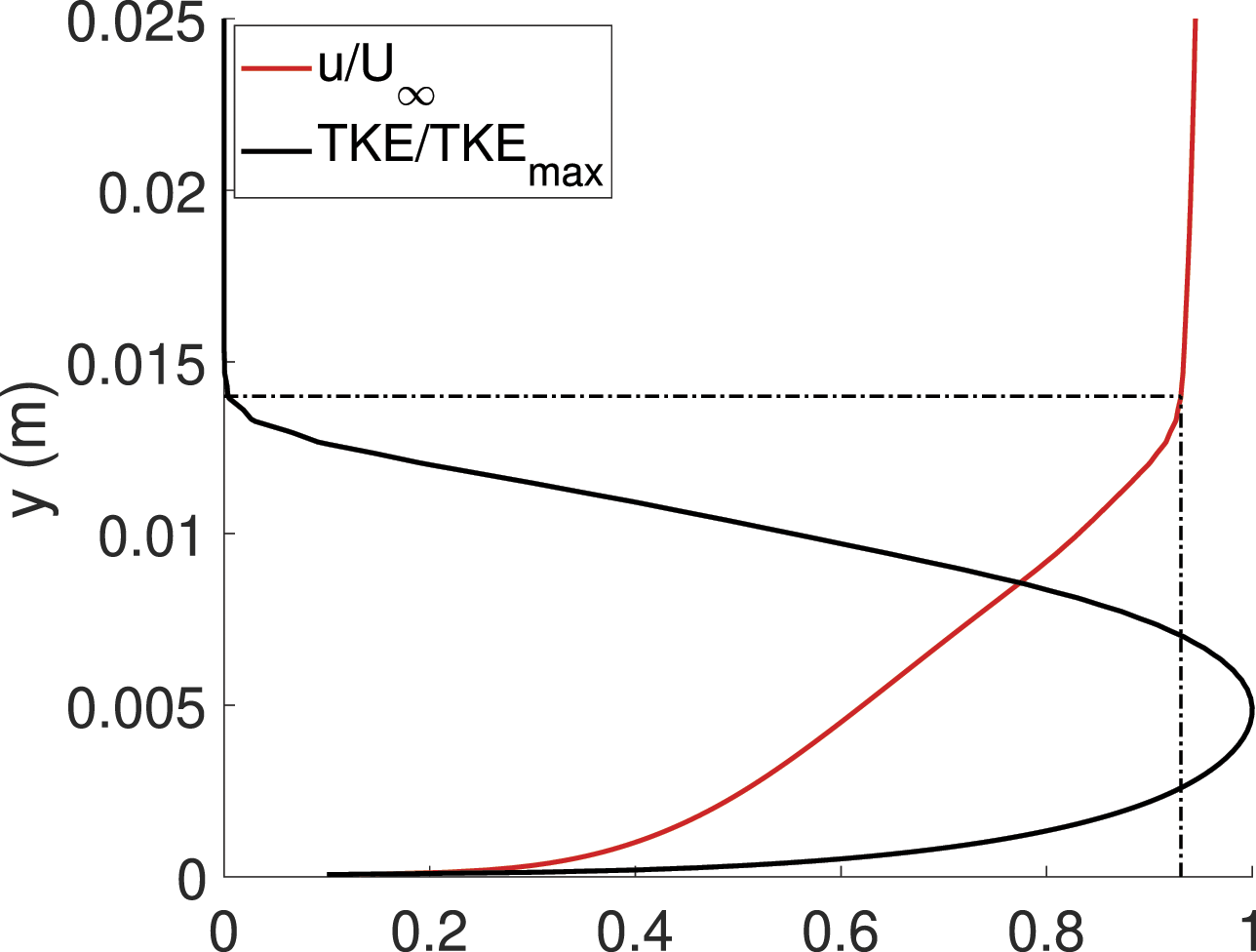

Trailing-edge noise predictions

Lee’s model¹⁹ is used to predict the wall pressure spectrum, Φ(ω), from the boundary layer input parameters as follows

\frac{Φ (ω) U_{e}}{τ_{w}^{2} δ^{*}} = \frac{max (a, (0.25 β_{c} - 0.52) a) {(ω δ^{*} / U_{e})}^{2}}{{[4.76 {(ω δ^{*} / U_{e})}^{0.75} + d^{*}]}^{e} + [8.8 R_{T}^{- 0.57} {(ω δ^{*} / U_{e})]}^{h^{*}}}

(1)

where τ_w is wall shear stress and β_c = (θ/τ_w) (dp/dx). The parameters a through h can be found in a reference¹⁹, in which Lee explicitly explains characteristics and derivations of these parameters.

Amiet’s trailing-edge noise model, modified by Roger and Moreau,^21,22 is then used to predict the sound pressure power spectral density, S_pp.

S_{p p} (\vec{x}, ω) = {(\frac{k c Z}{4 π S_{0}^{2}})}^{2} 2 Δ r | L |^{2} Φ (ω) l_{y} (ω, k_{y})

(2)

where ω is an angular frequency,

S_{0}^{2} = X^{2} + β^{2} (Y^{2} + Z^{2})

, X, Y, Z are the observer coordinates measured from an airfoil trailing edge, β² = 1 − M², M is a Mach number of flow, k is the acoustic wavenumber, c is the chord length, and Δr is the span.

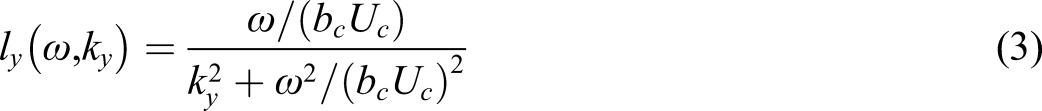
Corcos’ model²³ is used to calculate the spanwise correction length of the wall pressure spectrum, l_y(ω, k_y), as shown in equation (3)

l_{y} (ω, k_{y}) = \frac{ω / (b_{c} U_{c})}{k_{y}^{2} + ω^{2} / {(b_{c} U_{c})}^{2}}

(3)

where U_c = 0.7U_∞, k_y = 0, and b_c = 1.0 in this paper.

| L | is the loading function for trailing-edge noise, which is composed of two contributions: the trailing-edge scattering, L₁, and the leading-edge back-scattering, L₂. The leading-edge back-scattering is neglected in the current study. The trailing-edge scattering is defined as follows

L_{1} = - \frac{e^{2 i C}}{i C} {(1 + i) e^{- 2 i C} \sqrt{\frac{B}{B - C}} E^{*} [2 (B - C)] - (1 + i) E^{*} [2 B] + 1 - e^{- 2 i C} + \frac{e^{- 2 i C}}{4}}

(4)

where

B = \bar{K_{x}} + M_{0} \bar{μ} + \bar{κ}

(5)

C = \bar{K_{x}} - \bar{μ} (X / S_{0} - M_{0})

(6)

Further details of these formulations for the loading function can be found in a reference.²¹

Roger and Moreau’s modified Amiet’s thoery assumes the pressure near the edge is continuous and zero instead of the pressure jump, which is the assumption made in the original Amiet’s thoery. Roger and Moreau accounted for this assumption in their formulation by multiplying Amiet’s acoustic spectrum by a factor of four. Since the factor of four affects both the scattered and incident parts of the noise, Li and Lee²⁴ included an additional term so that the factor of four only affects the scattered part of the noise but not the incident part. The last term in equation (4) represents Li and Lee’s modification to Roger and Moreau’s formulation.

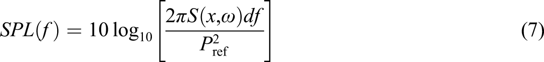
The resulting acoustic pressure is then used in equation (7) to compute sound pressure level, SPL(f), in a one-third octave band frequency spectrum.

S P L (f) = 10 \log_{10} [\frac{2 π S (x, ω) d f}{P_{ref}^{2}}]

(7)

where P_ref = 2 × 10⁻⁵.

Validation

Three validations are conducted prior to the detailed investigations into the effects of ice accretion on boundary layer flows and trailing-edge noise: airfoil trailing-edge noise predictions, ice accretion shape predictions, and iced airfoil CFD predictions. First, Benchmark Problems for Airframe Noise Computations (BANC) cases studied by Herr et al.²⁵ are replicated to validate airfoil trailing-edge noise predictions. Then, the experimentally obtained ice shapes presented in the article by Son et al.¹³ are used to validate LEWICE ice accretion models. Lastly, the work of Bragg et al.²⁶ is replicated to validate CFD predictions of pressure and flow fields as well as boundary layer parameters on an iced airfoil.

Airfoil trailing-edge noise validation

Amiet’s model in conjunction with Lee’s wall pressure spectrum model is validated against experimental data for trailing-edge noise. In addition, the pressure and skin friction coefficients are validated with the experimental data and XFOIL results, respectively. Table 1 shows four test cases, which exhibit a variation of the free-stream velocity and angle of attack. Trailing-edge noise is measured at 1 m distance from the trailing edge with 90°.

Table 1.

Benchmark problems for airframe noise computations conditions.

Cases	Airfoil	U_∞ (m/s)	ρ (kg/m³)	Re	α (°)	Chord (m)
BANC 1	NACA 0012	56.0	1.181	1.50 × 10⁶	0	0.4
BANC 2	NACA 0012	54.8	1.190	1.50 × 10⁶	4	0.4
BANC 3	NACA 0012	53.0	1.224	1.50 × 10⁶	6	0.4
BANC 4	NACA 0012	37.7	1.171	1.00 × 10⁶	0	0.4

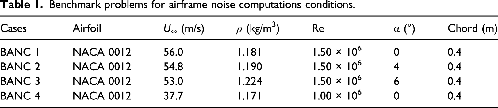
Figure 4 shows the pressure and skin friction coefficient plots as well as the streamwise velocity profile for BANC case 2. The CFD predictions show good agreement with the data or XFOIL results. We have confirmed that the CFD predictions maintain similar accuracy levels for the other three cases, but we do not show all those results for brevity of the paper.

Figure 4.

Benchmark problems for airframe noise computations case 2 CFD comparison with the measurement data²⁵: (a) pressure coefficient, (b) skin friction coefficient, and (c) streamwise velocity magnitude.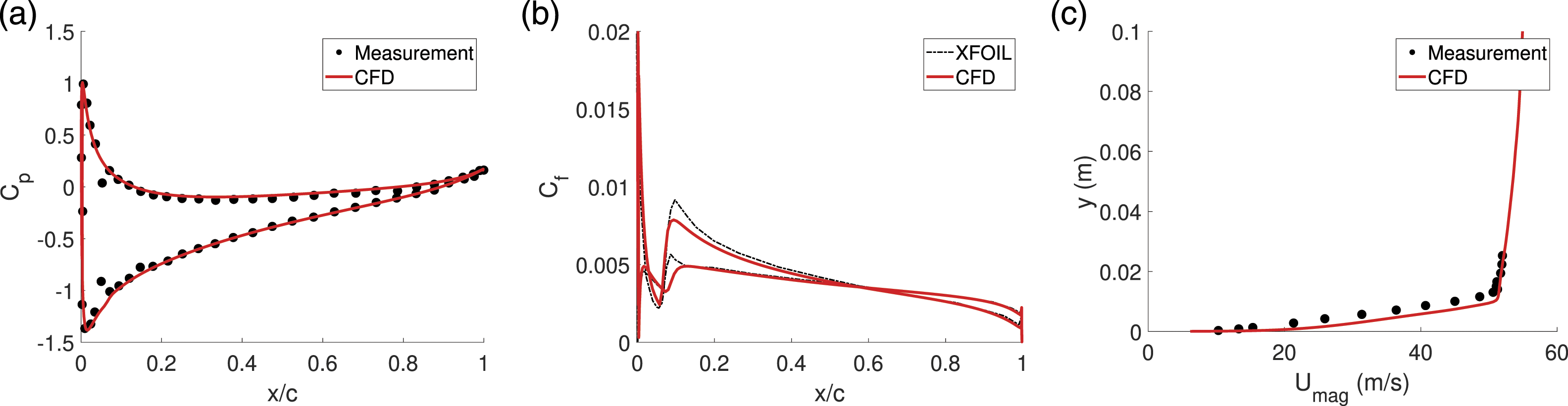

Figure 5 shows a comparison of trailing-edge noise between predictions and measurement data for four cases. It is found that the predictions are within ±3 dB difference from the measurement data, which is reported as the measurement uncertainty.²⁵ These results demonstrate the accuracy of trailing-edge noise predictions for both zero and non-zero angle of attack cases or adverse pressure gradient cases. The same approach was validated for trailing-edge noise of other airfoils as well.²⁷ It should be noted that the prediction approach is not limited to clean airfoils. As long as the boundary layer parameters, which are the inputs to the empirical wall pressure spectrum model, are accurately captured by CFD, the tool and method are applicable to any flow conditions or any airfoil shapes according to the wall pressure spectrum model.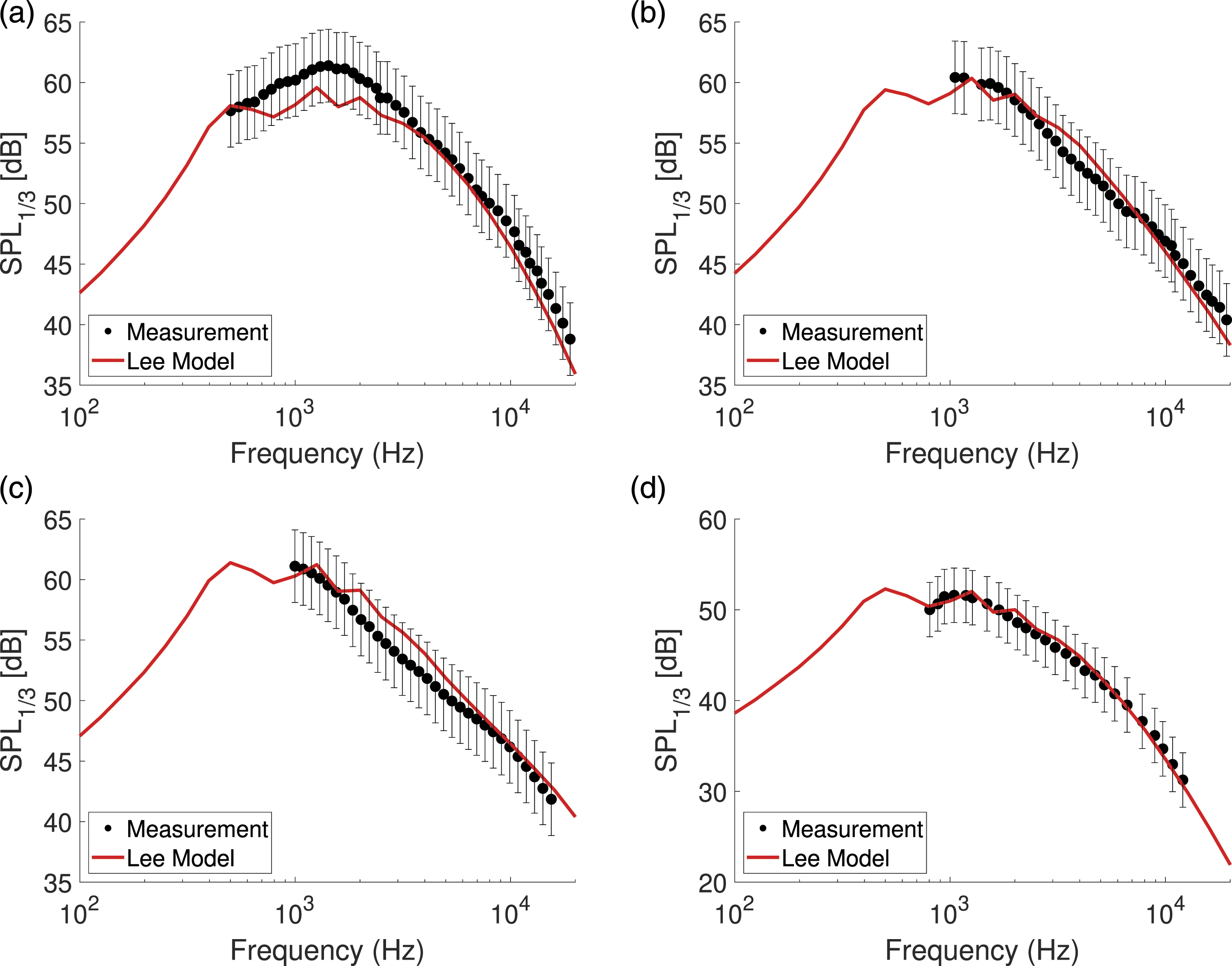

Figure 5.

Comparisons between the trailing-edge noise measurement data²⁵ and the predictions by Lee¹⁹ and Amiet’s²¹ model for Benchmark problems for airframe noise computations case 1 through 4: (a) case 1, (b) case 2, (c) case 3, and (d) case 4.

Ice accretion shape validation

LEWICE is used to predict ice accretion shapes and is validated against experimental data under different operating conditions. Table 2 shows three operating conditions. Case X is the rime icing condition, and Y and Z are the glaze icing conditions. A NACA0012 airfoil is used for all three cases. The angle of attack is 4°. The flow velocity is the same for cases X and Y, and it is slightly lower for case Z. In Table 2, TSTOP is the total icing accretion time.

Table 2.

Flow conditions of cases X, Y, and Z for ice shape validation.

Cases	α (°)	U_∞ (m/s)	T_∞ (°C)	LWC (g/m³)	MVD (μm)	TSTOP (s)
Case X	4	102.8	−22.8	0.55	20	400
Case Y	4	102.8	−11.1	0.60	15	384
Case Z	4	93.89	−12.2	1.05	20	372

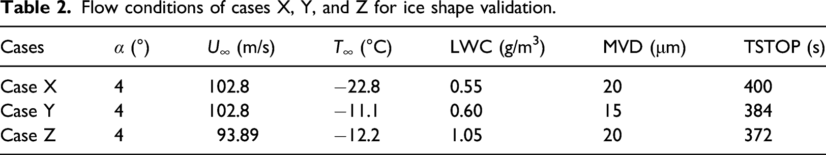
Figure 6 shows a comparison of the ice accretion shapes near the airfoil leading edge. The predicted ice shapes by LEWICE are compared with the measured shapes.^13,28 For reference, a clean airfoil is included in the figure. LEWICE predictions show excellent agreement for cases X and Y. Although the ice horn size on the lower side of case Z is under-predicted, the key characteristics of the ice shapes are well captured including the upper and lower horns.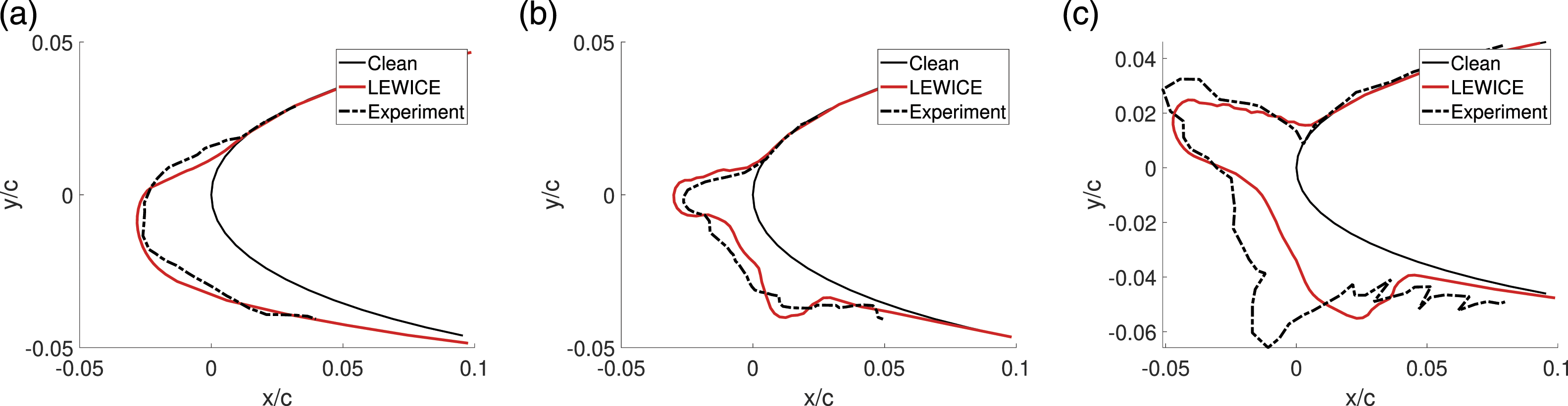

Figure 6.

LEWICE ice accretion shape validations against the experiment^13,28: (a) case X, (b) case Y, and (c) case Z.

Iced airfoil CFD validation

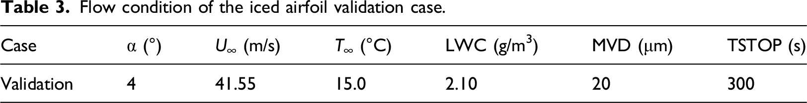
In this subsection, CFD predictions are validated against experimental data for a given iced shape. In particular, the leading-edge flow separation induced by an ice shape is highlighted, since this affects the development of turbulent boundary layer flows in downstream. The velocity profiles and boundary layer displacement and momentum thicknesses will be compared between CFD predictions and the measurement data at various chordwise distances. Figure 7(a) shows the zoom-in view of the airfoil leading edge. Clean and iced shapes are shown in the figure. The iced shapes are obtained from experiment,²⁶ and the corresponding flow condition is summarized in Table 3. A NACA0012 airfoil is used as a clean airfoil. Figure 7(b) shows that the ice-induced flow separation bubbles form behind the ice horns. The size of the flow separation bubble is determined by locating the flow separation and reattachment locations. The first location where the surface friction coefficient along the chord equals zero was considered the separation location. The following location after the separation, where the friction coefficient changes sign again, was considered the reattachment location. The normalized distance (x/c) between the flow separation and the reattachment locations is marked by the white lines in Figure 7(b) to indicate the size of the separation bubble.

Figure 7.

(a) Ice accretion shape and (b) velocity contour around the iced airfoil at α = 4°.

Table 3.

Flow condition of the iced airfoil validation case.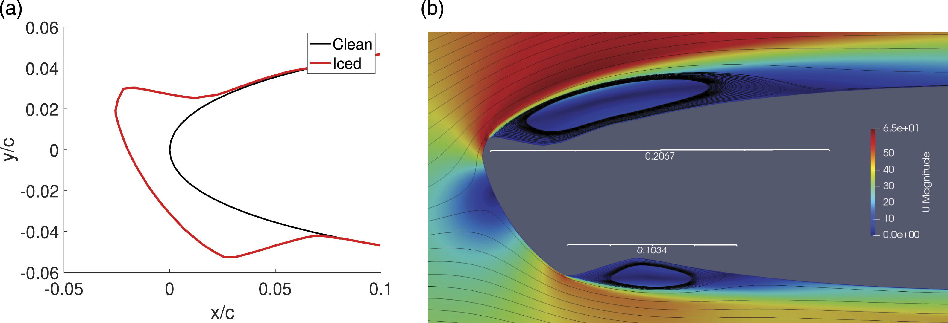

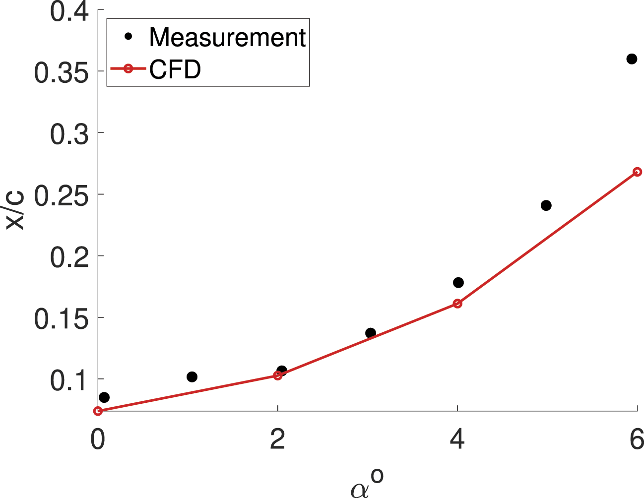
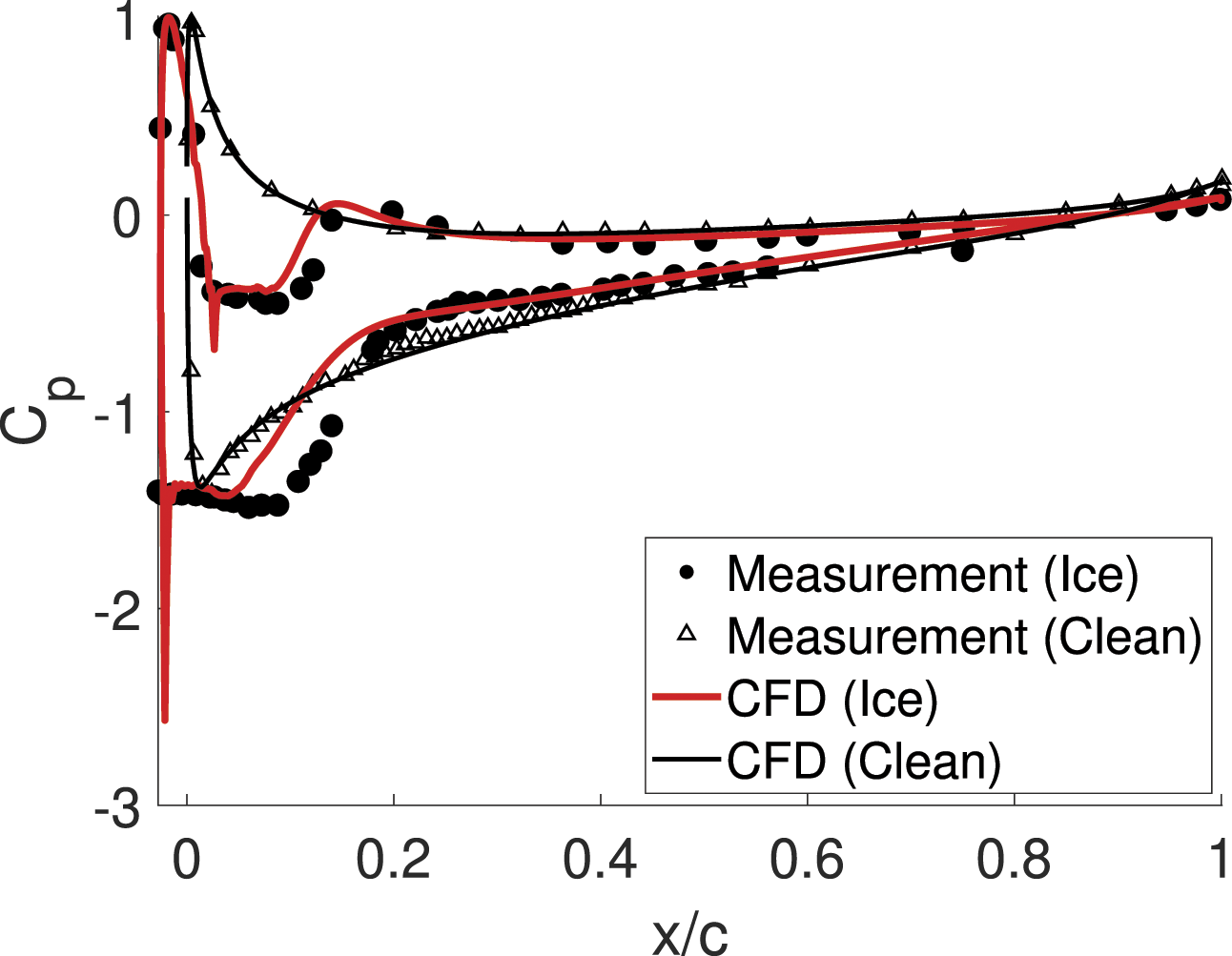
Case	α (°)	U_∞ (m/s)	T_∞ (°C)	LWC (g/m³)	MVD (μm)	TSTOP (s)
Validation	4	41.55	15.0	2.10	20	300

The comparison of the flow reattachment locations between the measurement data and CFD results as a function of angle of attack is shown in Figure 8 to demonstrate that CFD predicts the flow reattachment locations reasonably well. Although CFD loses its accuracy to predict the reattachment location at 6° angle of attack, its accuracy remains adequate until 4° angle of attack. Since the flow separation location is found to be the same for all angles of attack with the current validation case, the agreement of the reattachment location between the measurement and CFD results also indicates that the ice-induced separation bubble sizes are well predicted for angles of attack less than 6°. The size of the ice-induced flow separation bubble will be analyzed for different icing conditions in subsequent sections, which affect turbulent boundary layer development in downstream and trailing-edge noise. Figure 9 shows a comparison between the measurement and CFD results of the pressure coefficients for both the clean and iced airfoils. A CFD prediction of the clean airfoil pressure coefficient is in good agreement with the measurement data. The pressure drop due to the ice-induced flow separation near the leading edge and the pressure increase after reattachment are accurately captured by CFD.

Figure 8.

Comparison of the reattachment locations between the measurement and CFD predictions as a function of angle of attack.

Figure 9.

Validation of the pressure coefficient against the measurement data.²⁶

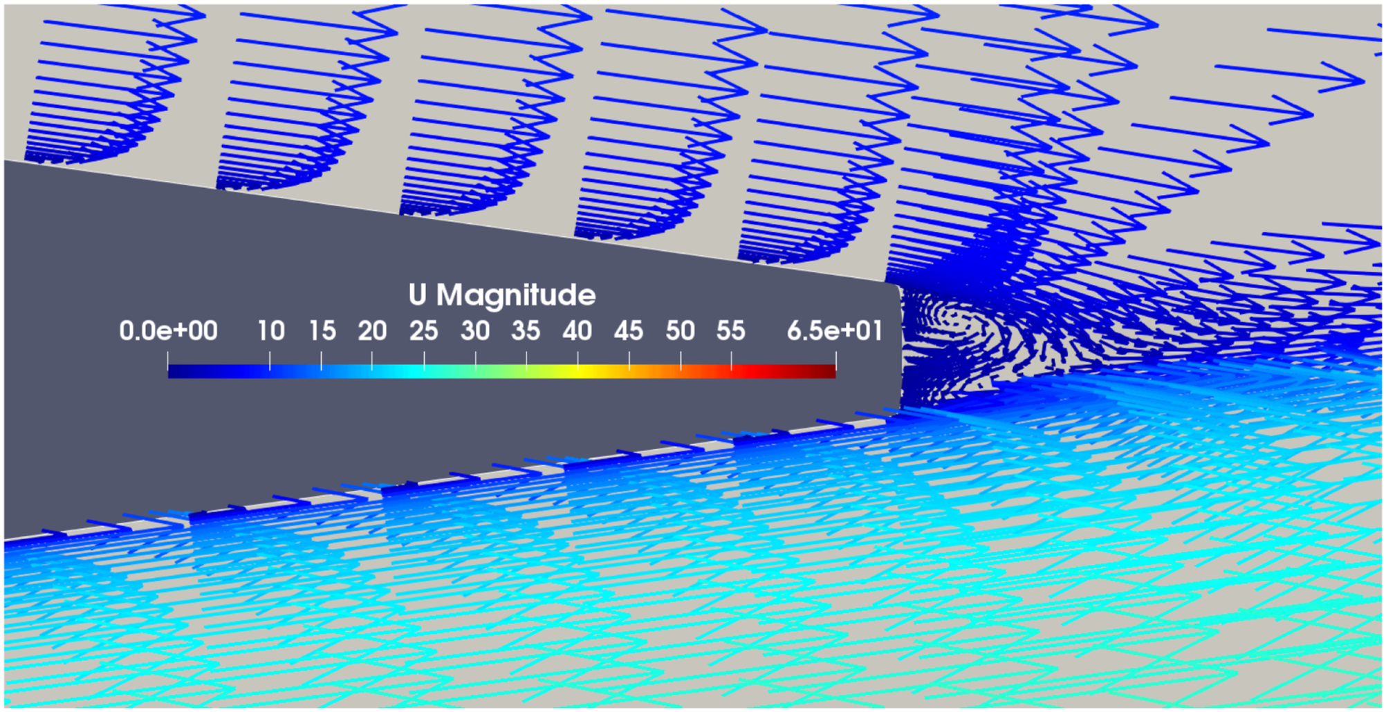
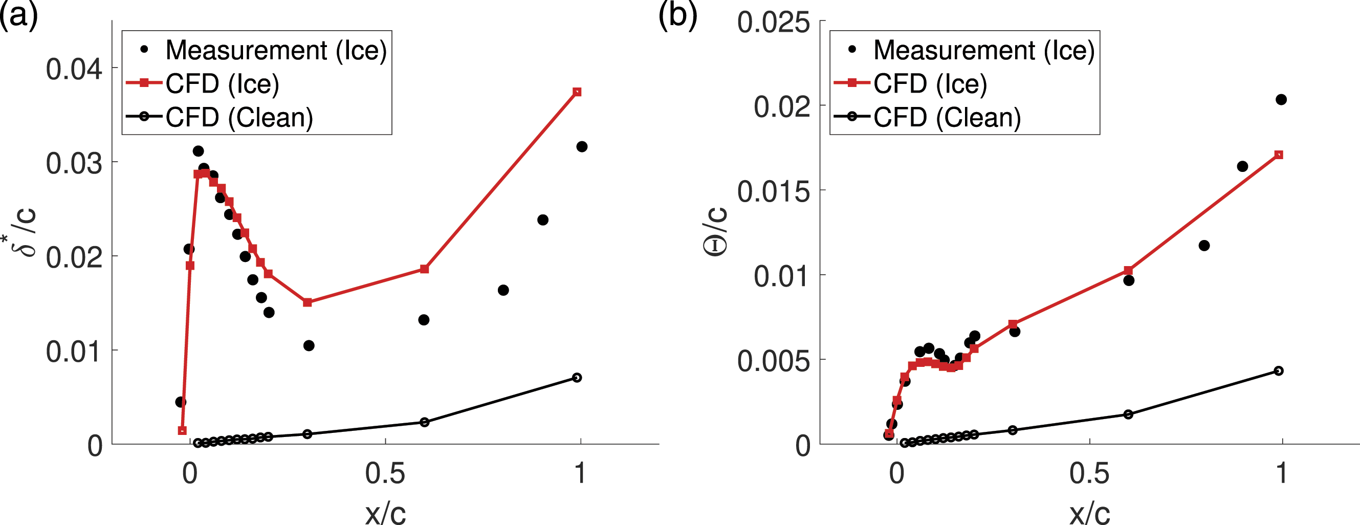
Since there are no available airfoil trailing-edge noise measurement data for this ice case, a noise validation is not conducted. However, since trailing-edge noise is predicted based on the boundary layer parameters obtained from CFD, it is reasonable to deduce that the noise prediction is valid as long as the boundary layer parameters are accurately estimated. Therefore, this subsection will focus on the boundary layer parameter predictions using CFD. Figure 10 shows the velocity profiles in the boundary layer at various chordwise locations near the leading edge. CFD predictions are compared with the data. It is found that the predictions match well with the measurement data, except in the range from 0 to 0.04c on the suction side. The flow separation is the strongest at 0.02c since the location is directly behind the ice. The thickness of the boundary layer mesh that was generated through Gmsh at this location is limited, so there could be more discrepancy between the measurement and the prediction, compared to the other locations along the chord. However, as we move farther downstream, the prediction matches better with the measurement. Since the trailing-edge noise is predicted based on the boundary layer parameters at 99% of the chord, the better match at downstream provides confidence in the velocity profile prediction near the wall in an important region. Figure 11 shows the velocity vector plot of this important region near the trailing edge. The velocity profiles inside the turbulent boundary layer near the trailing edge show that there is no flow separation on either side of the airfoil. The subsequent section will focus on the boundary layer parameters inside this turbulent boundary layer for the corresponding ambient condition case. Figures 12(a) and (b) show the boundary layer displacement and momentum thicknesses along the chord at α = 4°. For comparison, CFD predictions for a clean airfoil are included in each plot. It is shown that the iced airfoil dramatically increases the boundary layer displacement and momentum thicknesses, especially near trailing edge. Since the wall pressure spectrum is highly dependent on these parameters, it is fully expected that the iced airfoil would significantly alter the wall pressure spectrum and the resulting trailing-edge noise. It is found that the predicted displacement thickness is higher than the data from 0.3c to 1.0c. However, the trend is well captured in CFD: an increase after 0.4c. The comparison of the momentum thickness is much better. The trend as well as the absolute magnitude of the momentum thickness is well captured.

Figure 10.

Comparison between the measurement²⁶ and CFD results of the boundary layer velocity profiles at various locations along the chord: (a) suction side and (b) pressure side.

Figure 11.

Velocity vector plot of the iced airfoil for the CFD validation case near the trailing edge.

Figure 12.

Iced and clean airfoil CFD validations of boundary layer parameters against the measurement data²⁶ at α = 4°: (a) displacement thickness and (b) momentum thickness.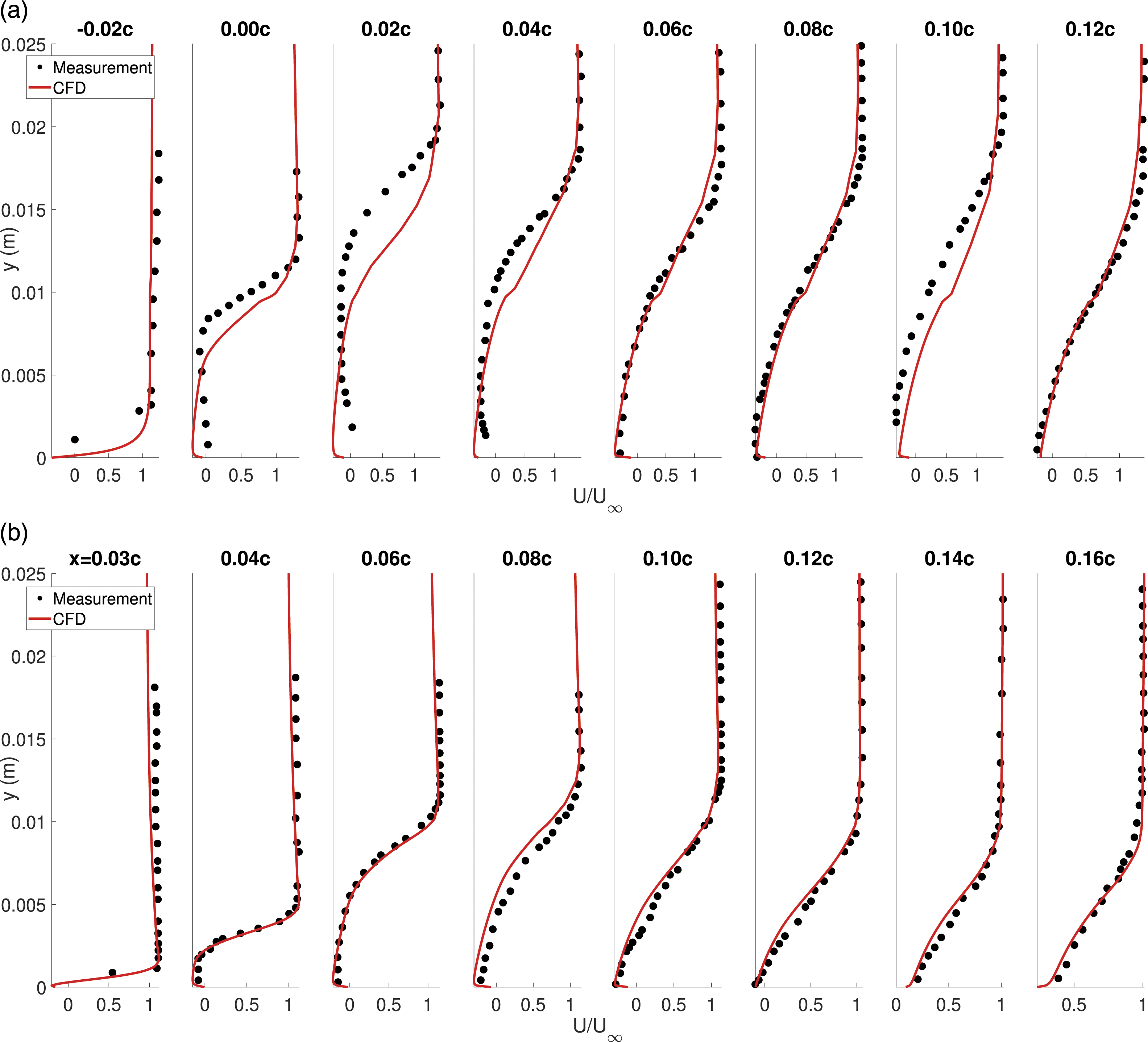

Results

Acoustic solver, LEWICE ice accretion model, and CFD were validated against experimental data in the previous section. In this section, we will use the validated tools to investigate the effect of flow and icing operating conditions, such as the flow velocity, temperature, LWC, MVD, and total time, on boundary layer parameters and the resulting trailing-edge noise. Table 4 shows all cases studied in this paper.¹³ In total, 31 cases are selected. Cases 1 vary LWC in a rime condition with a temperature of −20°C. The air density of 1.394 kg/m³ at −20°C and Reynolds number of 2.30 × 10⁶ are used for cases 1. Cases 2 vary LWC at a glaze condition with a temperature −5°C. The air density of 1.316 kg/m³ at −5°C and Reynolds number of 2.07 × 10⁶ are used for cases 2. Cases 3 vary the flow velocity at a rime condition, and the Reynolds number varies from 1.58 × 10⁶ to 6.16 × 10⁶ with the constant air density of 1.422 kg/m³ at − 25°C. Cases 4 vary the flow velocity at a glaze condition, and the Reynolds number varies from 1.42 × 10⁶ to 5.54 × 10⁶ with the constant air density of 1.341 kg/m³ at −10°C. Cases 5 vary the temperature from −3°C to −21°C, so the Reynolds number varies from 4.92 × 10⁶ to 5.57 × 10⁶ due to varying density at the corresponding ambient temperature. For all cases, a NACA0012 airfoil with the chord length of 0.5334 m at α = 4° is selected.

Table 4.

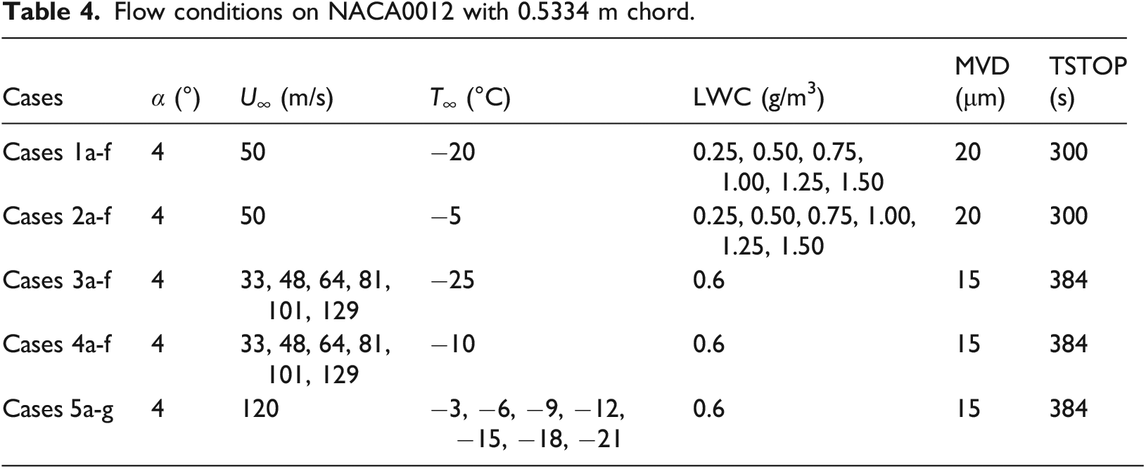
Flow conditions on NACA0012 with 0.5334 m chord.

Cases	α (°)	U_∞ (m/s)	T_∞ (°C)	LWC (g/m³)	MVD (μm)	TSTOP (s)
Cases 1a-f	4	50	−20	0.25, 0.50, 0.75, 1.00, 1.25, 1.50	20	300
Cases 2a-f	4	50	−5	0.25, 0.50, 0.75, 1.00, 1.25, 1.50	20	300
Cases 3a-f	4	33, 48, 64, 81, 101, 129	−25	0.6	15	384
Cases 4a-f	4	33, 48, 64, 81, 101, 129	−10	0.6	15	384
Cases 5a-g	4	120	−3, −6, −9, −12, −15, −18, −21	0.6	15	384

Cases 1: Varying liquid water content at a rime condition

Cases 1a through 1f are under a rime icing condition at − 20°C with varying LWC. Table 5 shows the boundary layer parameters for cases 1 at x/c = 0.99 on the suction side. Cases 1a-1e show very similar boundary layer characteristics, while case 1f exhibits a larger boundary layer thickness and the reduced pressure gradient. It indicates that the flow behavior is different for case 1f compared to the rest.

Table 5.

Varying liquid water content under a rime condition (cases 1): boundary layer parameters comparison (suction side).

Cases	U_e (m/s)	δ (m)	δ* (m)	θ (m)	C _f	dP/dx
1a	46.53	0.014001	0.003607	0.002159	0.000990	6867.0
1b	46.55	0.014001	0.003606	0.002161	0.000997	6851.2
1c	46.57	0.014668	0.003799	0.002260	0.000956	6720.3
1d	46.58	0.014668	0.003795	0.002255	0.000957	6697.3
1e	46.56	0.014668	0.003913	0.002311	0.000934	6548.5
1f	47.11	0.019668	0.005390	0.003092	0.000805	5513.4

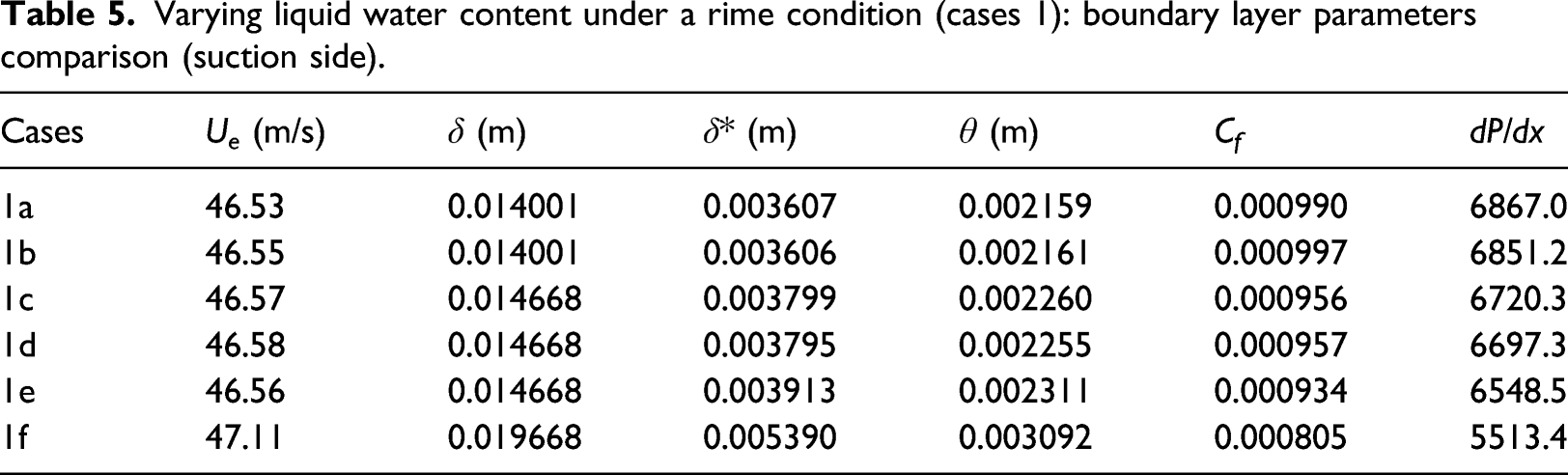
Figure 13(a) shows the ice shapes near the leading edge of the airfoil. A rime icing condition does not significantly alter the ice shapes until the LWC reaches 1.50 g/m³ (case 1f). The small ice horn developed at the leading edge in case 1f generates a significantly larger ice-induced separation bubble as shown in Figure 13(b). Only the suction side is presented for the ice-induced separation bubble measurement since the pressure side either does not have a bubble or the size is almost negligible so that they have little to no effect on the trailing-edge boundary layer flow characteristics. The boundary layer thickness in Figure 13(c) and the ice-induced separation bubble size in Figure 13(b) have the same trend, thus indicating that a larger bubble size contributes to a thicker boundary layer thickness as well as the displacement and momentum thicknesses. The turbulent kinetic energy (TKE) in Figure 13(d) also supports the increase in the boundary layer thickness with the development of the ice horn. It also indicates that the TKE magnitude becomes larger with the maximum TKE occurring farther away from the airfoil surface in case 1f, compared to the rest of the cases. A thick boundary layer thickness indicates a creation of larger turbulent eddies at the outer boundary layer region. The large turbulent eddies leave footprint of low- and mid-frequency pressure fluctuations on the wall according to the empirical wall pressure spectrum model or equation (1). Consequently, an increase in the low- and mid-frequency trailing-edge noise of case 1f is observed, while the rest of the cases do not exhibit notable changes in the noise level. This trend was also found in experimental data²⁵ and earlier study by Lee⁷: an increase in the boundary layer increases low- and mid-frequency trailing-edge noise.

Figure 13.

Boundary layer flow characteristics and trailing-edge noise under a rime condition with varying liquid water content: (a) ice accretion shapes, (b) ice-induced flow separation bubble size, (c) boundary layer, displacement, and momentum thicknesses at 99% chord on the suction side, (d) suction side TKE at 99% chord, and (e) trailing-edge noise comparison for cases 1a through 1f.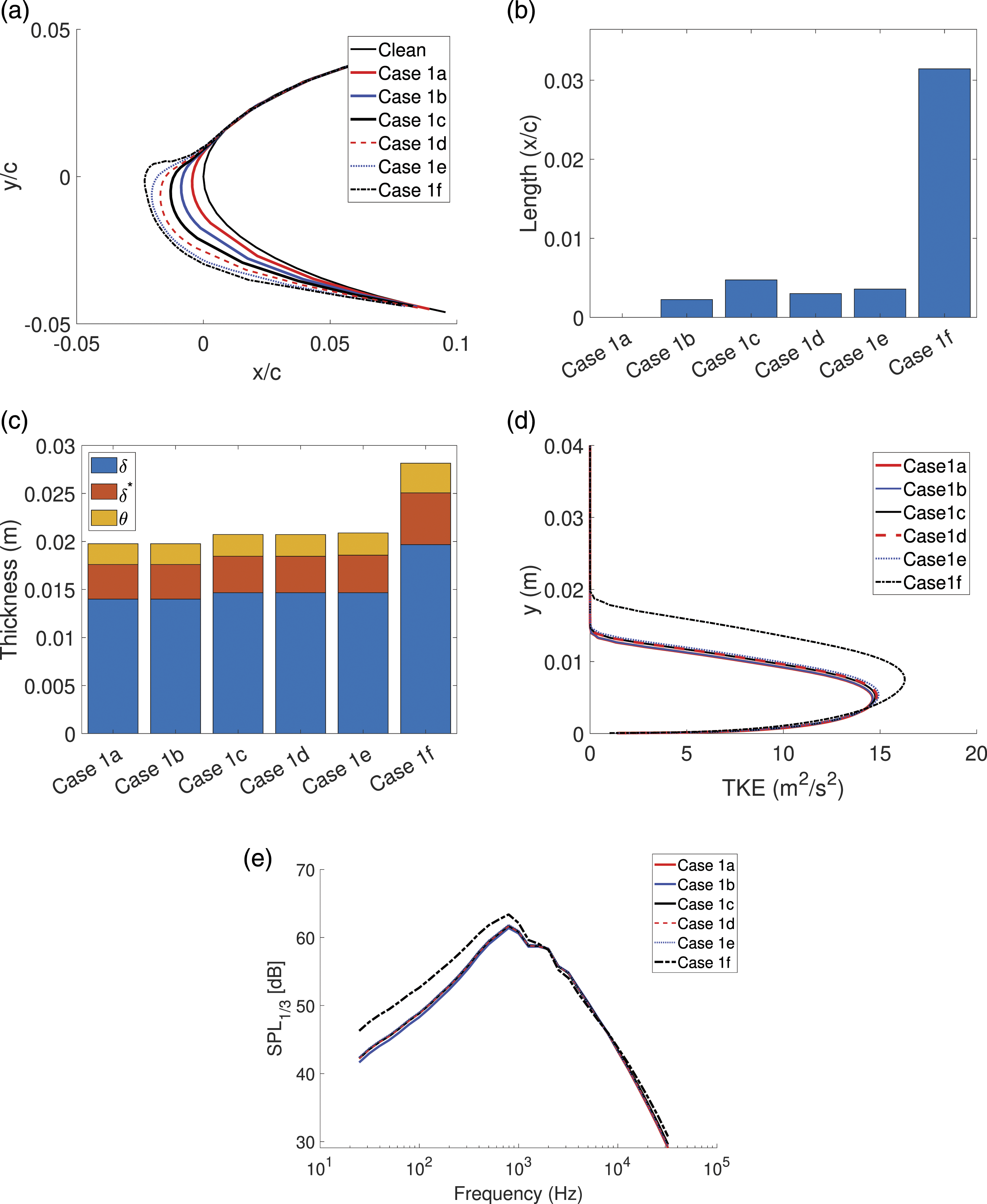

Cases 2: Varying liquid water content at a glaze condition

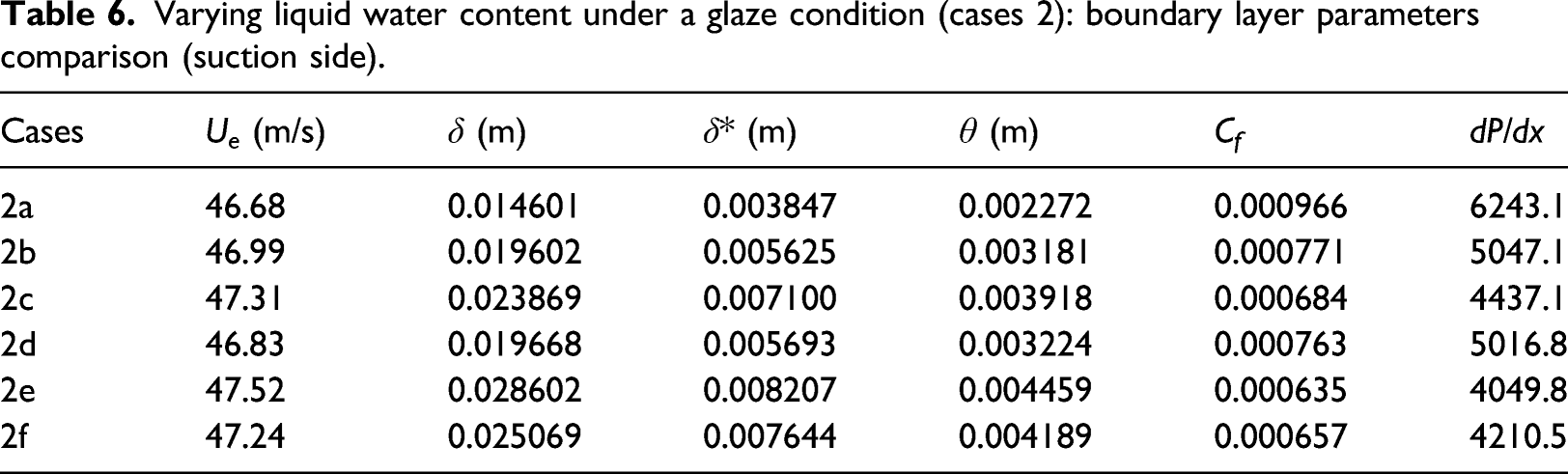
The ice shapes under a glaze icing condition, in contrast to those under a rime icing condition, are more irregular with horns developed at the leading edge. Figure 14(a) shows the development of the ice accretion as the LWC increases under a glaze icing condition. The ice shapes are more sensitive to the LWC variation under a glaze condition than those under a rime condition. Figure 14(b) shows the ice-induced separation bubble sizes as a result of varying LWC. The trend of the bubble sizes shows that LWC amount in the surrounding is not directly related to the size of the ice-induced separation bubble or the bubble size does not always increase as the LWC increases. Instead, the ice horn shape determines the size of the ice-induced separation bubble behind the horn. Then, the size of the bubble affects the turbulent flow development along the airfoil surface, resulting in an increase in the boundary layer, displacement, and momentum thicknesses at the trailing edge (99% chord) as shown in Fig. 14(c). TKE comparison among cases 2 in Figure 14(d) shows that the location where the maximum TKE occurs shifts upward and the TKE magnitude increases with increasing the boundary layer thicknesses.

Figure 14.

Boundary layer flow characteristics and trailing-edge noise under a glaze condition with varying liquid water content: (a) ice accretion shapes, (b) ice-induced flow separation bubble size, (c) boundary layer, displacement, and momentum thicknesses at 99% chord on the suction side, (d) suction side TKE at 99% chord, and (e) trailing-edge noise comparison for cases 2a through 2f.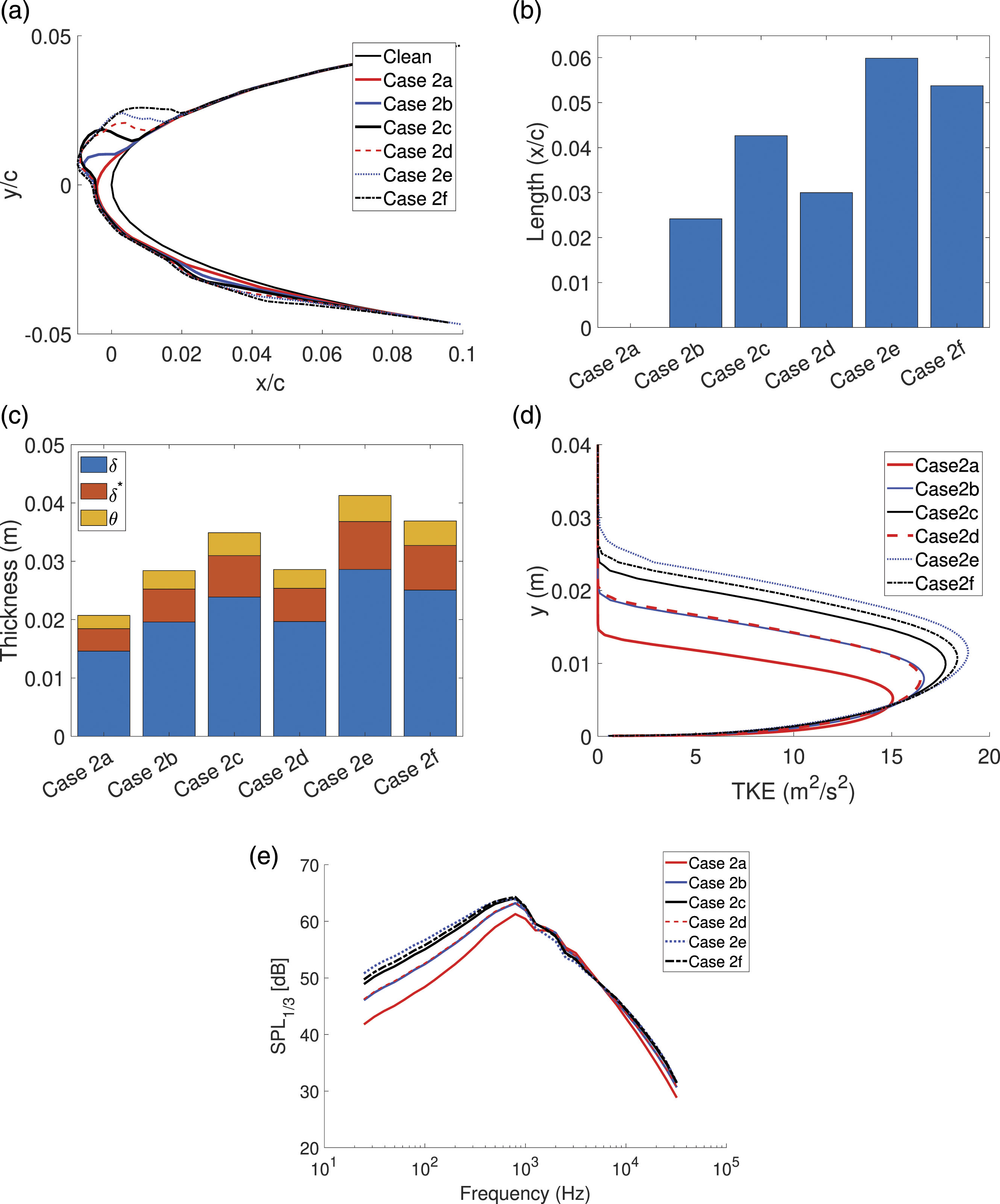

Similar to the previous results from cases 1, an increase in the low- and mid-frequency trailing-edge noise is observed as the boundary layer thickness increases. Figure 14(e) shows that the noise level in case 2e is higher than that in case 2f and the noise level in case 2c is higher than that in case 2d. This trend is consistent with that observed in the Figures 14(b) and (c). In other words, the noise amplitude results directly resemble the separation bubble size. All six boundary layer parameters on the suction side under a glaze icing condition are tabulated in Table 6 for an easier numerical comparison between the cases 2. The reduction of the pressure gradient is observed for the cases with increasing the boundary layer thicknesses, and the increase in the pressure gradient is observed for the cases with decreasing the boundary layer thicknesses.

Table 6.

Varying liquid water content under a glaze condition (cases 2): boundary layer parameters comparison (suction side).

Cases	U_e (m/s)	δ (m)	δ* (m)	θ (m)	C _f	dP/dx
2a	46.68	0.014601	0.003847	0.002272	0.000966	6243.1
2b	46.99	0.019602	0.005625	0.003181	0.000771	5047.1
2c	47.31	0.023869	0.007100	0.003918	0.000684	4437.1
2d	46.83	0.019668	0.005693	0.003224	0.000763	5016.8
2e	47.52	0.028602	0.008207	0.004459	0.000635	4049.8
2f	47.24	0.025069	0.007644	0.004189	0.000657	4210.5

Cases 3: Varying freestream velocity at a rime condition

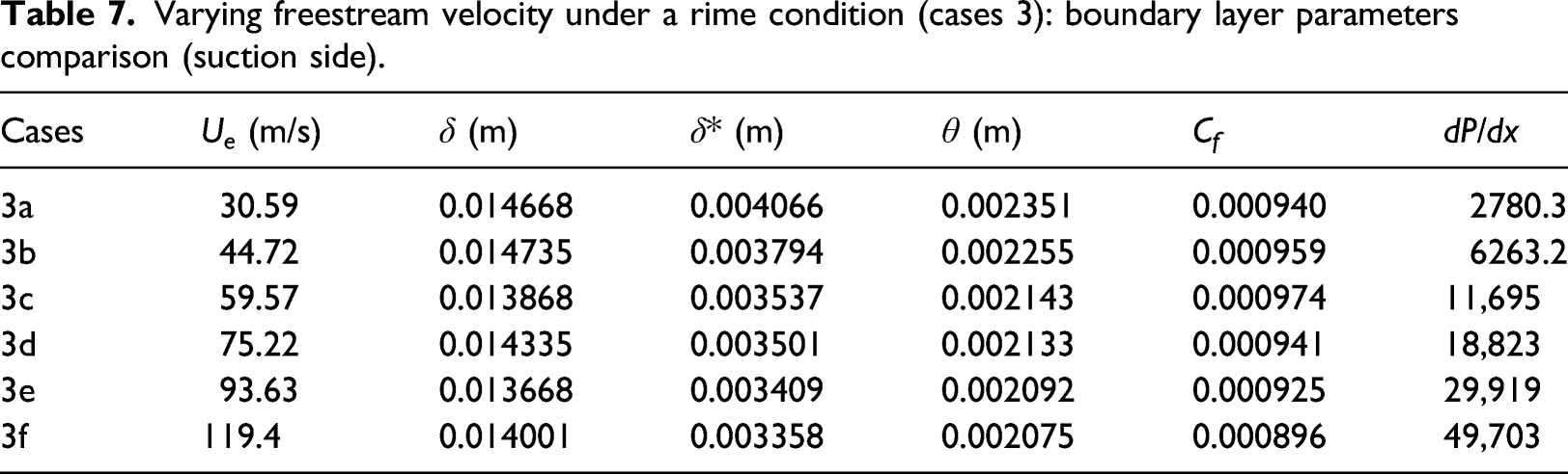
In cases 3, the freestream velocity is varied under a rime icing condition. As shown in Table 4, LWC is maintained constant at 0.6 g/m³, MVD is reduced to 15 μm, and the exposure time (TSTOP) is increased to 384 s, compared to the icing conditions for cases 1 and 2. Figure 15(a) shows the development of the ice accretion as the freestream velocity increases. The ice shapes under a rime ice condition grow in the upstream direction with increasing the velocity, and no ice horns are developed at all velocities. The upstream ice accretion does not induce significant flow separation. Figure 15(b) shows ice-induced flow separation bubble sizes. It should be noted that the bubble sizes are very small to have any significant impact on the boundary layer flow characteristics at the trailing edge. This is evident by the boundary layer thicknesses shown in Figure 15(c), in which no significant variations in the thicknesses are observed. Although the boundary layer thickness does not change noticeably, the TKE magnitude inside the turbulent boundary layer in Figure 15(d) increases with increasing the freestream velocity. As a result of the increasing TKE inside the fairly constant boundary layer throughout cases 3, the trailing-edge noise shown in Figure 15(e) exhibits an increase in the noise level at all frequency spectrum with the peak noise level shifting to the higher frequency region. Table 7 shows the boundary layer parameters on the suction side. It is clear that the edge velocity increases with the freestream velocity. As the edge velocity increases, the magnitude of the wall pressure spectrum increases with the peak frequency shifting to high frequencies according to the empirical wall pressure spectrum model or equation (1). The pressure gradient at 99% chord also increases with the freestream velocity despite the development of ice accretion. Overall, the effect of the change in the freestream velocity on the boundary layer parameters and trailing-edge noise is much larger than that of the ice accretion shapes.

Figure 15.

Boundary layer flow characteristics and trailing-edge noise with varying freestream velocity at T_∞ = −25°C: (a) ice accretion shapes, (b) ice-induced flow separation bubble size, (c) boundary layer, displacement, and momentum thicknesses at 99% chord on the suction side, (d) suction side TKE at 99% chord, and (e) trailing-edge noise comparison for cases 3a through 3f.

Table 7.

Varying freestream velocity under a rime condition (cases 3): boundary layer parameters comparison (suction side).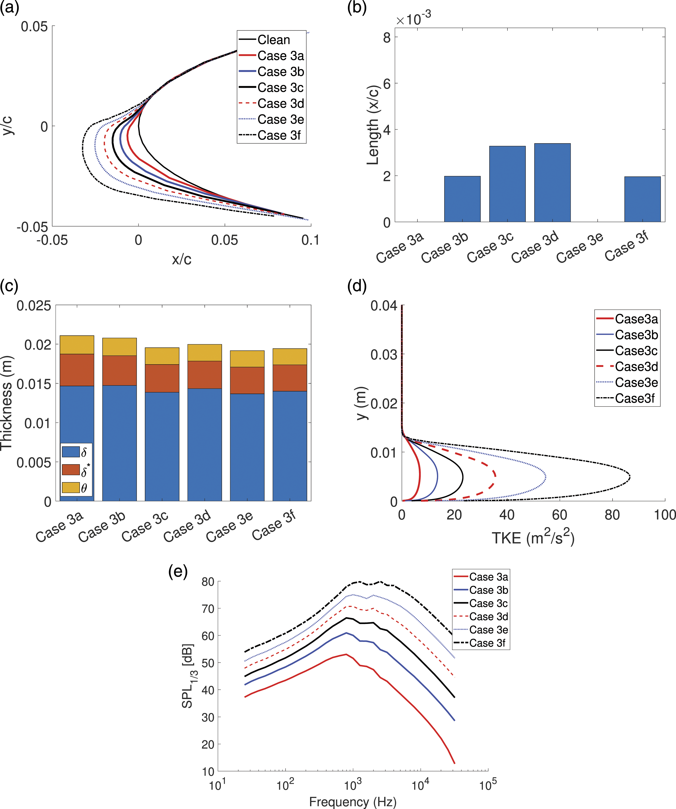

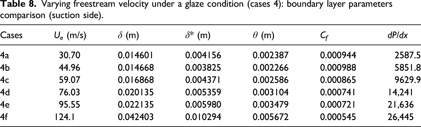
Cases	U_e (m/s)	δ (m)	δ* (m)	θ (m)	C _f	dP/dx
3a	30.59	0.014668	0.004066	0.002351	0.000940	2780.3
3b	44.72	0.014735	0.003794	0.002255	0.000959	6263.2
3c	59.57	0.013868	0.003537	0.002143	0.000974	11,695
3d	75.22	0.014335	0.003501	0.002133	0.000941	18,823
3e	93.63	0.013668	0.003409	0.002092	0.000925	29,919
3f	119.4	0.014001	0.003358	0.002075	0.000896	49,703

Cases 4: Varying freestream velocity at a glaze condition

Unlike cases 3, the ice shapes in cases 4 are more sensitive to the change in the freestream velocity under a glaze icing condition. Figure 16(a) shows the growth of ice accretion as velocity increases.

Figure 16.

Boundary layer flow characteristics and trailing-edge noise with varying freestream velocity at T_∞ = −10°C: (a) ice accretion shapes, (b) ice-induced flow separation bubble size, (c) boundary layer, displacement, and momentum thicknesses at 99% chord on the suction side, (d) suction side TKE at 99% chord, and (e) trailing-edge noise comparison for cases 4a through 4f.

The first ice horn is developed on the upper surface when the freestream velocity reaches 64 m/s. Another horn is developed on the lower surface when the velocity reaches 81 m/s. Once developed, these horns grow in size with increasing the velocity. As a result of the continuously increasing ice horn size, the ice-induced separation bubble sizes shown in Figure 16(b) also increase. Figure 16(c) shows that the boundary layer thicknesses significantly increase along with the ice-induced separation bubble sizes. The TKE comparison among cases 4 in Figure 16(d) shows the increase in magnitude as well as the upward shift of the location where the maximum TKE occurs. The increase in the freestream velocity increases TKE magnitude, while the thickening of the boundary layer causes the maximum TKE location to move farther away from the airfoil surface. However, the pressure gradient in Table 8 does not follow the trend previously observed in cases 1 and 2; instead, pressure gradient increases despite the ice accretion. This observation indicates that the effect of the freestream velocity on the pressure gradient is more important than the effect of the ice-induced separation bubble. It is also clearly seen that the boundary layer edge velocity increases with the freestream velocity, which affects the noise level and peak frequency. Figure 16(e) shows that the trailing-edge noise increases evenly over all frequency spectrum under a glaze icing condition due to a combination of two effects: the freestream or boundary layer edge velocity that increases high-frequency noise and the boundary layer thickness that increases low-frequency noise. It has been shown that in cases 2, the ice shapes increase low- and mid-frequency noise as the larger ice horns are formed. Then, in cases 3, the increase in the high-frequency noise is observed due to the increasing freestream velocity while the ice shapes have a minimal impact on the trailing-edge noise. Since cases 4 vary ice shapes and the freestream velocity, they show the combined effect of the ice shape changes and the increasing freestream velocity on the trailing-edge noise. As a result, the peak noise level does not noticeably shift to the higher frequency region with increasing velocity unlike the trend shown previously in Figure 15(e). Therefore, an increase in the freestream velocity under a glaze icing condition evenly raises the noise level over the entire frequency range.

Table 8.

Varying freestream velocity under a glaze condition (cases 4): boundary layer parameters comparison (suction side).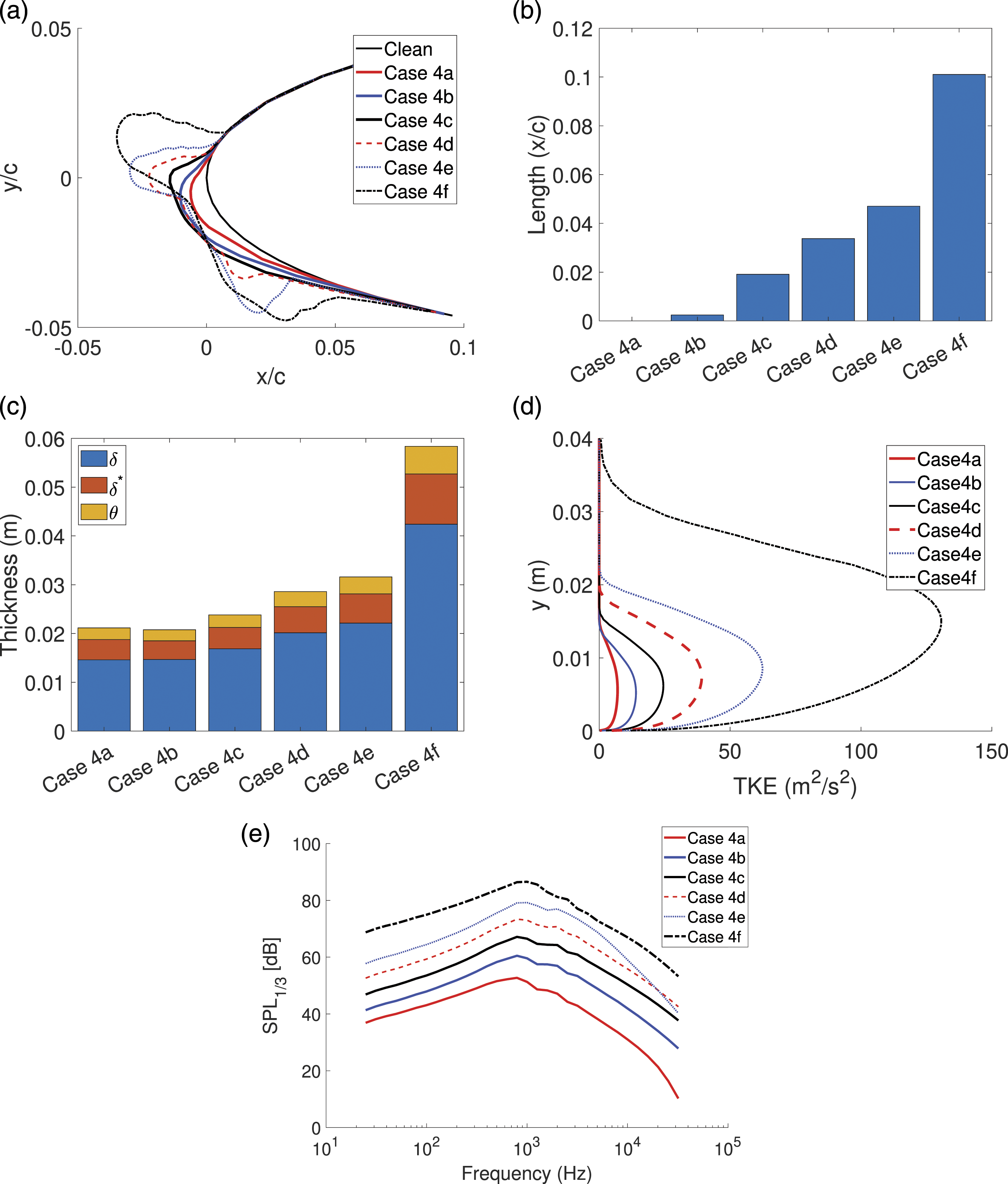

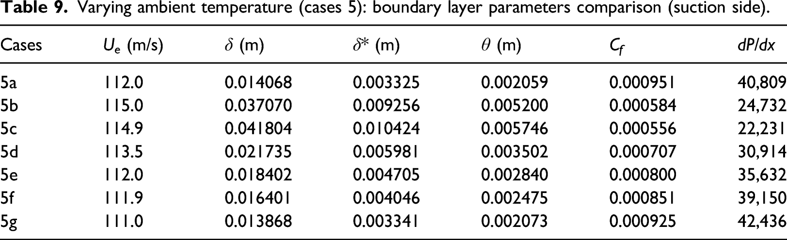
Cases	U_e (m/s)	δ (m)	δ* (m)	θ (m)	C _f	dP/dx
4a	30.70	0.014601	0.004156	0.002387	0.000944	2587.5
4b	44.96	0.014668	0.003825	0.002266	0.000988	5851.8
4c	59.07	0.016868	0.004371	0.002586	0.000865	9629.9
4d	76.03	0.020135	0.005359	0.003104	0.000741	14,241
4e	95.55	0.022135	0.005980	0.003479	0.000721	21,636
4f	124.1	0.042403	0.010294	0.005672	0.000545	26,445

Cases 5: Varying ambient temperature

Finally, the ambient temperature is varied in cases 5 to investigate the effect of ice accretion on the boundary layer flow characteristics and the resulting trailing-edge noise under various ambient temperatures. Here, the freestream velocity, LWC, MVD, and TSTOP are maintained constant at 120 m/s, 0.6 g/m³, 15 μm, and 384 s, respectively.

Figure 17(a) shows an evolution of ice accretion as the ambient temperature decreases from −3°C to −21°C. An ice horn is developed on the upper surface at − 6°C (case 5b), and this ice horn moves upstream towards the leading edge as the temperature further decreases until it eventually becomes a streamwise ice accretion in case 5g. From the previous cases, the ice shapes were shown to be more irregular under a glaze icing condition; this trend conforms with the trend observed in Figure 17(a) since the most notable irregular ice shapes occur between −6°C and −12°C. Figure 17(b) shows the resulting ice-induced separation bubble sizes. It is worthwhile to note that the size of the bubble in cases 5a and 5g is negligible despite the difference between the amount of ice accumulated at the leading edge. At a temperature close to zero, not enough ice accretes at the leading edge to generate an ice-induced flow separation; on the other hand, at a very cold temperature, or a rime icing condition, a streamwise ice shape is formed with no visible horns, thus generating a negligible flow separation bubble. Consequently, the boundary layer thicknesses of cases 5a and 5g shown in Figure 17(c) are similar. Table 9 also exhibits numerical results of the boundary layer parameters, which show negligible differences in the boundary layer thicknesses between cases 5a and 5g. From the rest of the cases (5b through 5f), it is clear that the larger ice horns induce more flow separations behind the horns, which increases the boundary layer thickness at the trailing edge. However, as the ice horns move upstream along with decreasing the ambient temperature, the size of the ice-induced flow separation bubbles reduces as well as the boundary layer thickness. A large variation of the TKE profile is observed with decreasing the ambient temperature in Figure 17(d). When the flow separation bubble sizes are large, such as cases 5b and 5c, the TKE magnitudes are also large compared to the rest of the cases. With the ice accretion developing upstream, the flow near the trailing edge is less perturbed, resulting in the decrease in the TKE magnitude and the maximum TKE location closer to the airfoil surface. The resulting trailing-edge noise shown in Figure 17(e) exhibits the same trend: the thicker boundary layer thickness contributes to the increase in the low- and mid-frequency noise. Cases 5a and 5g have almost identical sound pressure levels (SPLs) because their boundary layer parameters are similar. An increase in the low- and mid-frequency noise is greatest in case 5c since the larger eddies inside the thickened boundary layer interacting with the surface near the trailing edge contribute more to the low- and mid-frequency noise. For the same reason, as the boundary layer thickness increases from cases 5f to 5b, the low- and mid-frequency noise also increases.

Figure 17.

Boundary layer flow characteristics and trailing-edge noise with varying ambient temperature: (a) ice accretion shapes, (b) ice-induced flow separation bubble size, (c) boundary layer, displacement, and momentum thicknesses at 99% chord on the suction side, (d) suction side TKE at 99% chord, and (e) trailing-edge noise comparison for cases 5a through 5g.

Table 9.

Varying ambient temperature (cases 5): boundary layer parameters comparison (suction side).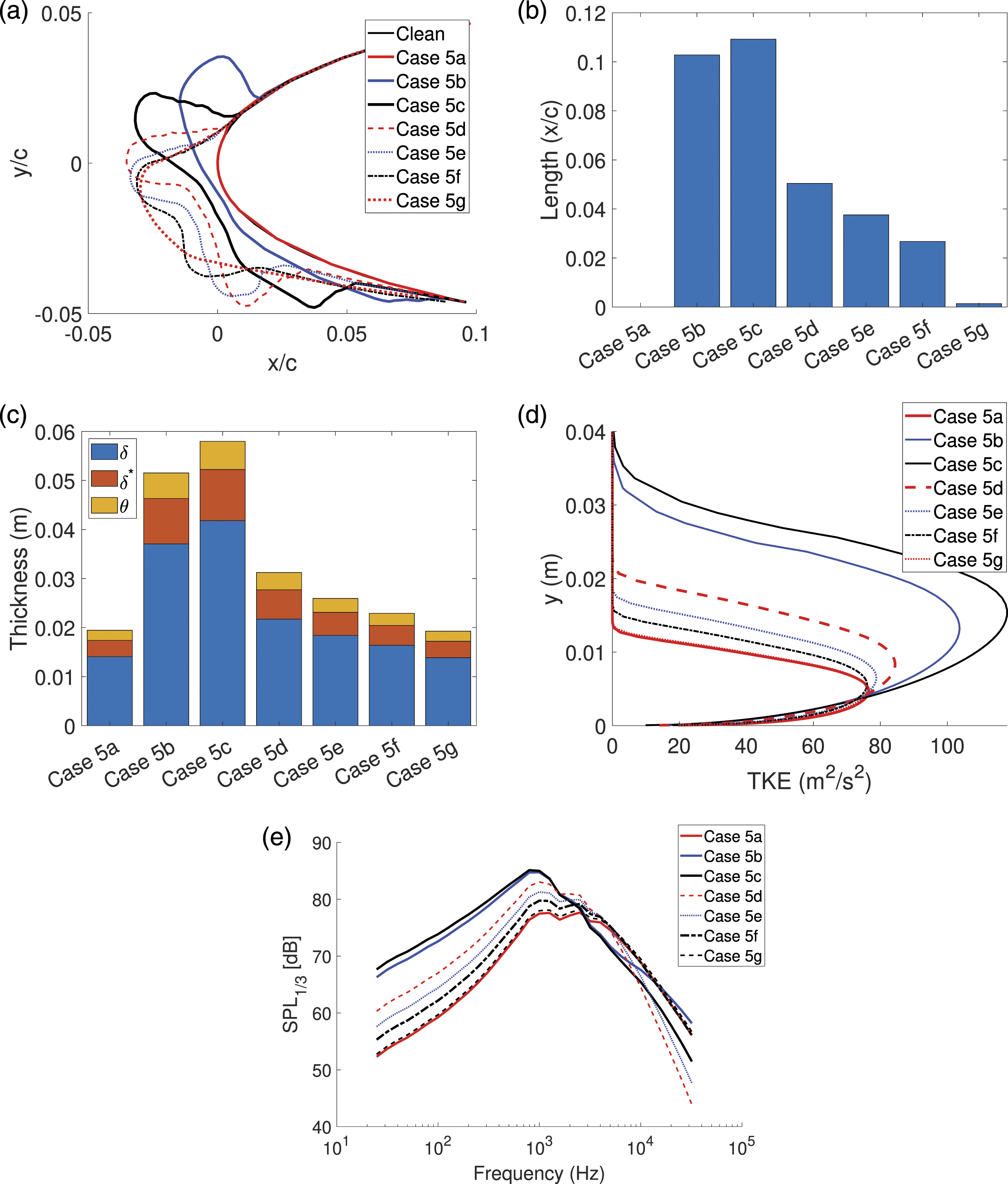

Cases	U_e (m/s)	δ (m)	δ* (m)	θ (m)	C _f	dP/dx
5a	112.0	0.014068	0.003325	0.002059	0.000951	40,809
5b	115.0	0.037070	0.009256	0.005200	0.000584	24,732
5c	114.9	0.041804	0.010424	0.005746	0.000556	22,231
5d	113.5	0.021735	0.005981	0.003502	0.000707	30,914
5e	112.0	0.018402	0.004705	0.002840	0.000800	35,632
5f	111.9	0.016401	0.004046	0.002475	0.000851	39,150
5g	111.0	0.013868	0.003341	0.002073	0.000925	42,436

Directivity

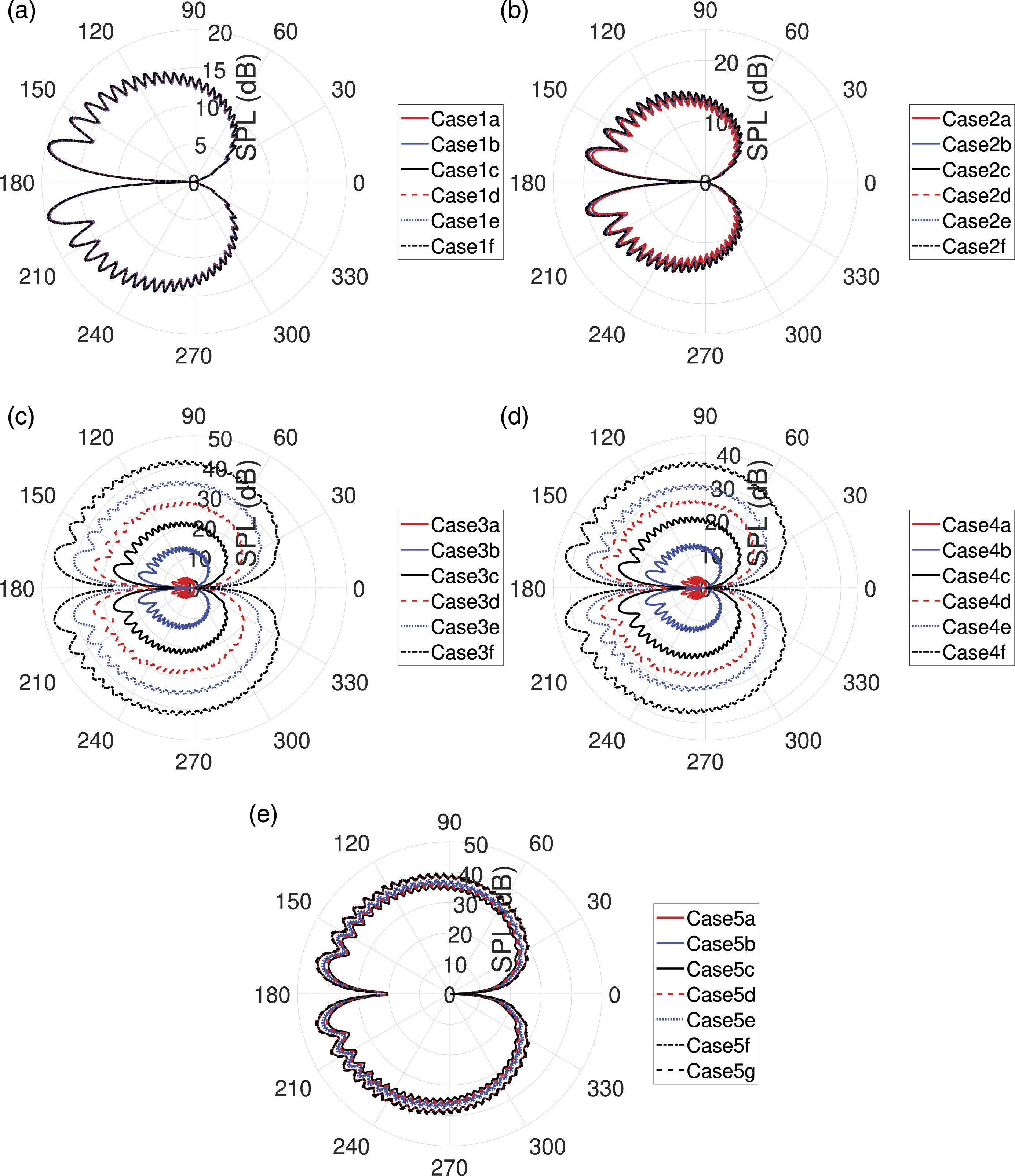
In the previous section, we used only a single observer that is located 1 m away from trailing edge. In order to complete the analysis, we investigate the noise directivity surrounding the airfoil in this subsection. Figures 18 and 19 show directivity plots of all cases for frequencies at 500 Hz and 8000 Hz, respectively. The observer location is chosen at 1 m away from the trailing edge. It should be noted that the directivity plots represent narrow band SPL values, while the previous results represent one-third octave band SPL values. The low-frequency directivity plots show dipole sound radiation patterns and the high-frequency directivity plots show cardioid sound radiation patterns toward the leading edge with many minor lobes as expected by the nature of the trailing-edge noise propagation. Although the angle of attack of 4° was used to study the trailing-edge noise directivity, the shapes of the dipoles are symmetric about the horizontal axis. This is because Amiet’s trailing-edge noise model that was used to obtain directivity plots assumes zero degree angle of attack. Note that the flow was rotated with 4° angle of attack while keeping the airfoil geometry fixed. The directivity plots at low and high frequencies for all cases clearly resemble the relationship between ice accretion and the trailing-edge noise that was previously observed. For instance, Figure 18(a) shows that the directivity plot of case 1f at low frequency has a larger magnitude compared to the rest of cases 1. However, Figure 19(a) shows that the directivity plots of all cases have the same magnitude at high frequency, which resembles the noise prediction results shown in Figure 13(e). The comparison between Figures 18 and 19 further demonstrates that ice accretion impacts more in the low-frequency region than the high-frequency region, except cases 3 and 4 where noise increases at both frequencies.

Figure 18.

Directivity plots at 500 Hz: (a) cases 1a-1f, (b) cases 2a-2f, (c) cases 3a-3f, (d) cases 4a-4f, and (e) cases 5a-5g.

Figure 19.

Directivity plots at 8000 Hz: (a) cases 1a-1f, (b) cases 2a-2f, (c) cases 3a-3f, (d) cases 4a-4f, and (e) cases 5a-5g.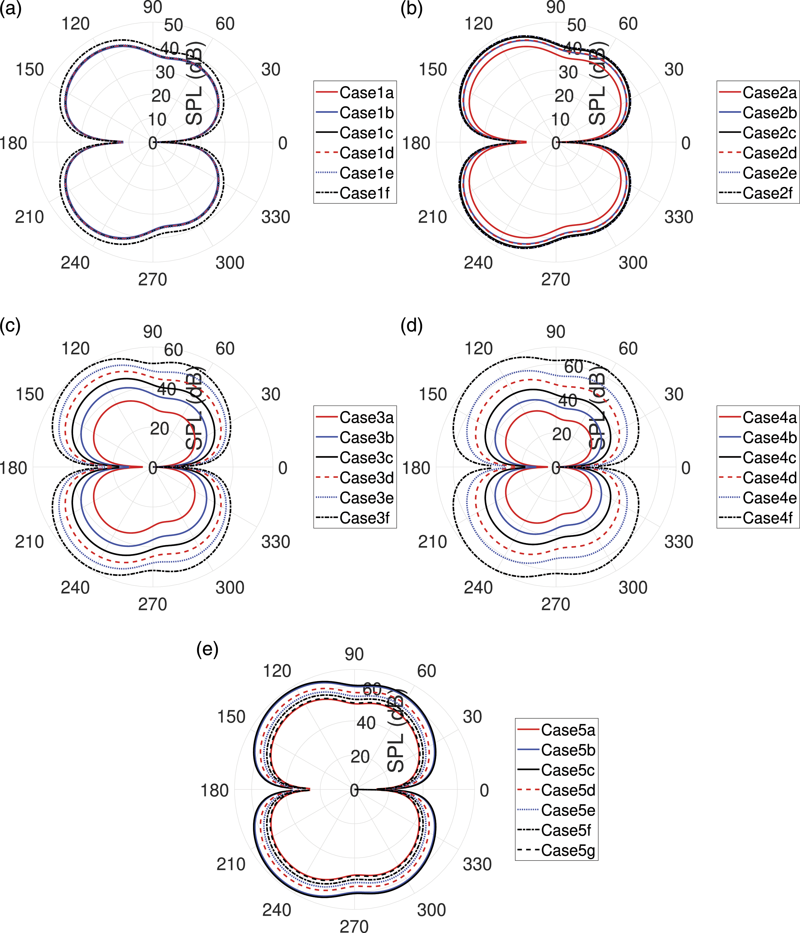

Conclusion

In this paper, we investigated the effect of 2-D ice accretion on turbulent boundary layer flows and trailing-edge noise. It was demonstrated that the accreted ice shape at the leading edge plays a critical role in changing the boundary layer flow parameters, which significantly affect the trailing-edge noise. Flow conditions were varied to observe how the ice accretion and noise responded to LWC, freestream velocity, and ambient temperature. The followings are concluded from the results:

1. The shape of the ice accretion is most sensitive to the variables at temperatures between T = −6°C and T = −12°C, or a glaze icing condition.

2. An increase in LWC does not necessarily increase the ice-induced flow separation bubble. Rather, the size of the ice horn or the severity of ice shape deformation contributes to the bubble sizes.

3. Ice accretion that forms in the upstream direction or the streamwise ice accretion has minor impacts on the boundary layer characteristics at the trailing edge.

4. A larger ice-induced flow separation bubble increases the boundary layer thickness, displacement thickness, and momentum thickness at the trailing edge.

5. Thicker boundary layer, displacement, and momentum thicknesses caused by the larger ice-induced separation bubbles increase trailing-edge noise in low- and mid-frequency ranges.

6. A higher free-stream velocity increases the noise levels and shifts the peak frequency to high frequency at rime conditions, but it increases the noise levels more evenly without the shift of the peak frequency at glaze conditions.

7. Directivity plots confirm the dipole acoustic radiation at low frequency and the cardioid radiation pattern at high frequency. In general, the ice accretion affects more to the magnitude of the dipole directivity at low frequency except the cases where the freestream velocity changes.

These results provide important insights on how ice accretion shapes are affected by the flow conditions and how the boundary layer flow at the trailing edge is impacted by the resulting ice shapes. We note that our simulations and results were made at one ice exposure time. Although ice accretion is a dynamic process, understanding how turbulent boundary layer and trailing-edge noise are affected by the ice shape under a steady state condition (instant moment at the end of the given exposure time) provides insights into dynamic changes of the noise characteristics during the exposure time. It has been shown that the ice shapes that induce large flow separation increases low- and mid-frequency noise. During the ice accretion process, the low- and mid-frequency trailing-edge noise would increase as the ice horn grows larger. However, during the streamwise ice development, the trailing-edge noise may not vary noticeably even in the dynamic process.

As another limitation, the ice-induced roughness was not considered in this paper since the fully developed ice shapes after a long period of exposure time are considered. However, the ice-induced roughness is important during the early stage of ice accretion, which may cause changes in the ice shapes and thus resulting trailing-edge noise. In this case, the noise predictions can be further improved by employing a roughness model to account for the ice roughness when estimating ice accretion shapes in early stage. Although the test cases are limited to one airfoil and one angle of attack, the trends observed in the boundary layer and noise predictions as a result of ice accretion would remain the same for the similar icing cases. Ultimately, understanding these flow physics behind noise generation due to ice accretion would be beneficial to noise-sensitive industries, such as aviation and wind turbine power generation.

Footnotes

Acknowledgements

The authors would like to acknowledge Inbal Shlesinger for her support on generating ice geometry using LEWICE.

Declaration of conflicting interests

The author(s) declared no potential conflicts of interest with respect to the research, authorship, and/or publication of this article.

Funding

The author(s) received no financial support for the research, authorship, and/or publication of this article.

ORCID iDs

Hyunjune Gill

Seongkyu Lee

References

Brooks

Pope

Marcolini

. Aifoil Self-Noise And Prediction. VA, USA: NASA RP 1218, 1989.

Lee

Ayton

Bertagnolio

, et al. Turbulent boundary layer trailing-edge noise: theory, computation, experiment, and application. Prog Aerospace Sci 2021; 126: 100737. DOI: 10.1016/j.paerosci.2021.100737

Oerlemans

Sijtsma

Méndez López

. Location and quantification of noise sources on a wind turbine. J Sound Vibration 2007; 299: 869–883. DOI: 10.1016/j.jsv.2006.07.032

Lee

. Prediction of rotorcraft broadband trailing-edge noise and parameter sensitivity study. J Am Helicopter Soc 2020; 65: 1–14. DOI: 10.4050/JAHS.65.042006

Lee

. Prediction of Urban air mobility multirotor VTOL broadband noise using UCD-QuietFly. J Am Helicopter Soc 2021; 66: 1–13. DOI: 10.4050/JAHS.66.032004

Lee

. Acoustics analysis of a quiet helicopter for air taxi operations. Virtual Event. In: 77th VFS International Annual Forum.

Lee

. The effect of airfoil shape on trailing edge noise. J Theor Comput Acoust 2019; 27(2): 1850020. DOI: 10.1142/S2591728518500202

Liu

Lee

. Parametric airfoil design and sensitivity analysis for turbulent boundary-layer trailing-edge noise reduction. AIAA J 2022; 60: 2324–2341. DOI: 10.2514/1.J060096

Kelly

Habashi

Quaranta

, et al. Ice accretion effects on helicopter rotor performance, via multibody and cfd approaches. J Aircraft 2018; 55(3): 1165–1176. DOI: 10.2514/1.C033962

10.

McKillip

Jr Kaufman

Quackenbush

. evtol accretion modeling for supporting algorithmic icing detection. Virtual Event. In: Vertical Flight Society’s 76th Annual Forum and Technology Display.

11.

Scroger

Palacios

Han

. Empirical modeling of urban air mobility rotor icing thrust degradation. Virtual Event. In: AIAA Aviation 2020 Forum.

12.

Blasco

Palacios

Schmitz

. Effect of icing roughness on wind turbine power production. Wind Energy 2016; 20: 601–617. DOI:10.1002/we.2026

13.

Son

Yee

. Quantitative analysis of a two-dimensional ice accretion on airfoils. J Mech Sci Techn 2012; 26(4): 1059–1071. DOI: 10.1007/s12206-012-0223-z

14.

Morelli

Zhou

Guardone

. Acoustic characterization of glaze and rime ice structures on an oscillating airfoil via fully unsteady simulations. J Am Helicopter Soc 2020; 65(4): 1–12. DOI: 10.4050/JAHS.65.042004

15.

Cheng

Han

Brentner

, et al. Surface roughness effect on rotor broadband noise. Int J Aeroacoustics 2018; 17(4–5): 438–466. DOI: 10.1177/1475472X18778278

16.

Wright

. User Manual for the NASA Glenn Ice Accretion Code LEWICE Version 2.0. Brook Park, Ohio: Dynacs Engineering Company, Inc., 1999.

17.

Geuzaine

Remacle

J-F

. Gmsh: A 3-D finite element mesh generator with built-in pre- and post-processing facilities. Int J Numer Methods Eng 2009; 79(11): 1309–1331. DOI: 10.1002/nme.2579

18.

Weller

Tabor

Jasak

, et al. A tensorial approach to computational continuum mechanics using object-oriented techniques. Comput Phys 1998; 12(6): 620. DOI: 10.1063/1.168744

19.

Lee

. Empirical wall-pressure spectral modeling for zero and adverse pressure gradient flows. AIAA J 2018; 56(5): 1818–1829. DOI: 10.2514/1.J056528

20.

Catlett

Anderson

Forest

, et al. Empirical modeling of pressure spectra in adverse pressure gradient turbulent boundary layers. AIAA J 2016; 54(2): 569–587. DOI: 10.2514/1.J054375

21.

Roger

Moreau

. Extensions and limitations of analytical airfoil broadband noise models. Int J Aeroacoustics 2010; 9(3): 273–305. DOI: 10.1260/1475-472X.9.3.273

22.

Lee

. Predictions and validations of small-scale rotor noise using ucd-quietfly. In: Proceedings of the American Helicopter Society Technical Conference on Aeromechanics Design for Transformative Vertical Flight, San Jose, CA, 25–27 January 2022.

23.

Corcos

. The structure of the turbulent pressure field in boundary-layer flows. J Fluid Mech 1964; 18(3): 353–378. DOI: 10.1017/S002211206400026X

24.

Lee

. Analytic prediction of rotor broadband noise with serrated trailing edges. In: Proceedings of the Vertical Flight Society 78th Annual Forum & Technology Display, Fort Worth, Texas, USA, 10–14 May 2022.

25.

Herr

Ewert

Rautmann

, et al. Broadband Trailing-Edge Noise Predictions - Overview of Banc-Iii Results. Dallas, TX: AIAA/CEAS 21st Aeroacoustics Conference. AIAA Paper 2015-2847.

26.

Bragg

Khodadoust

Spring

. Measurements in a leading-edge separation bubble due to a simulated airfoil ice accretion. AIAA J 1992; 30(6): 1462–1467. DOI: 10.2514/3.11087

27.

Lee

Shum

. Prediction of airfoil trailing-edge noise using empirical wall-pressure spectrum models. AIAA J 2019; 57(3): 888–897. DOI: 10.2514/1.J057787

28.