Noise shielding of a deflected flap for comparing numerical predictions with flyover experiments

Abstract

Comparing acoustic simulations against experimental data is an essential step in order to prove the correctness of numerical tools. This can be done with wind tunnel experiments where the environmental conditions can be adjusted very accurately. Ultimately, the tools must be capable of predicting real-word scenarios like aircraft flyovers. However, obtaining precise data from flyover experiments is challenging and often important input data is missing. The current paper shows, that by extracting the shielding effect of a small detail, a deflecting flap of an aircraft with rear-mounted engines, it is possible to reproduce flyover measurements with a boundary element method, even when only little engine information is known. The boundary element method can only take a constant mean flow into account, but by additionally evaluating results of a volume-resolved discontinuous Galerkin method more insights into the expected effects of a realistic mean flow is given.

Introduction

One of the major goals for future aircraft is the significant reduction of noise. Europe’s vision for aviation Flightpath 2050 ¹ defines the goal that “The perceived noise emission of flying aircraft is reduced by 65%” compared to a typical new aircraft in 2000. It is expected that such a goal can only be achieved by a revolutionary change of aircraft design. A vital step for such designs is to place the engines above the wing or even the fuselage such that most noise is shielded by the airframe. The prediction of noise immission on the ground, which is caused by such configurations is difficult due to limited experience. Only first-principles based high-fidelity methods can be regarded as reliable candidates for such configurations. Still, these methods must prove their reliability.

Recent research by Rossignol et al.^2,3 using wind tunnel experiments are showing that numerical methods can accurately predict shielding effects including detailed interference patterns. When it comes to flyover measurements, the validation procedure is more difficult, since repeatability is much harder to achieve and the exact source strengths cannot easily be quantified. Besides, in order to compute shielding two different configurations must be measured (e.g., isolated source against installed source) which is much more difficult to realize in flyover experiments compared to wind tunnel experiments.

Alves Vieira et al. ⁴ recently published an analysis of engine shielding based on flyover measurements comparing different aircraft types with different engine positions. Compared to configurations with engines under the wing, they where able to show that aircraft with rear-mounted engines expose decreased noise levels where wing and fuselage are shielding the engine noise. They also present that shielding predictions with numerical methods are possible but difficult especially since their measurement data come from real-life airport operation where there are large fluctuations between different flyovers.

More accurate flyover measurement data can obtained by defining laboratory conditions using remote airports and research aircraft which can repeat predefined settings many times. Such studies under the context of noise reduction treatments were e.g. conducted by Yamamoto at al. ⁵ Another impressive study with more than 1000 flyovers spanning over several years was recently published by Khorrami et al. ⁶ By using numerical simulations they were able to reproduce the basic effects of the installed noise reductions devices.

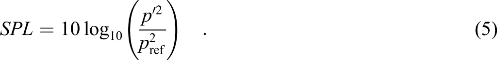
The flyover experiments on which the present paper is based on can be categorized in-between the previously mentioned works. On the one hand, a research aircraft is being used for obtaining high-quality data but on the other hand a very limited amount of flyovers was conducted without any noise reduction treatments. The experiment is tailored to determine shielding effects by using an aircraft with rear-mounted engines where the fan noise is partly shielded by the wing. See Figure 1 for a rough sketch of the configuration and the rough area of where the engine noise is shielded. Even though the flyover study was limited to only a few flyovers, careful evaluation of the data provides accurate data which can be compared to the results of acoustic prediction methods. More precisely, the amount of extra shielding when deflecting the flap (which means increasing the wing shielding area) is compared to simulation results.

Figure 1.

Sketch of HALO research aircraft with wing shadow region for noise emitted from the engine inlet.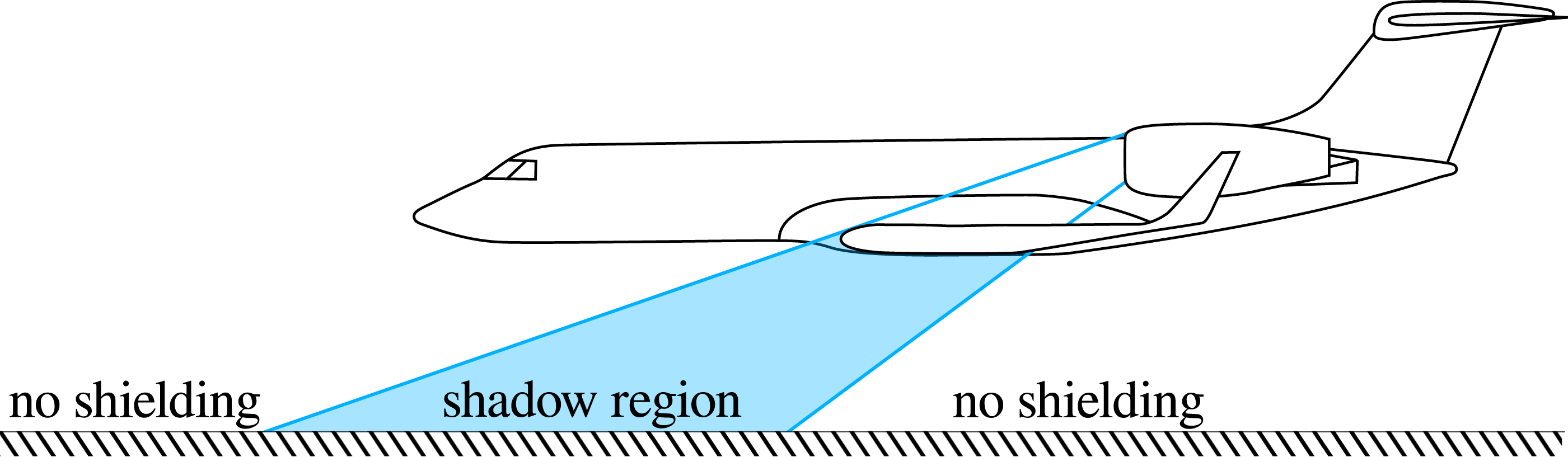

Two high-fidelity methods will be applied within this paper. The first method is a boundary element method (BEM) accelerated with a fast multipole algorithm. With little computational efforts this method is able to predict the trends of noise shielding when deflecting the flap. Since this method cannot take a realistic mean flow into account, but only a spatially uniform mean flow at moderate Mach numbers a second method is used in order to give insights into the errors made. This second method is a volume resolving solver using a discontinuous Galerkin (DG) scheme, which can consider the detailed flow around the aircraft including boundary layers. However, the solution process is computationally very demanding and the application had to be restricted to low frequencies far below the first blade passing frequency. This means that the mean flow effects are only analyzed theoretically at low frequencies without direct comparisons to the experimental data.

Case setup

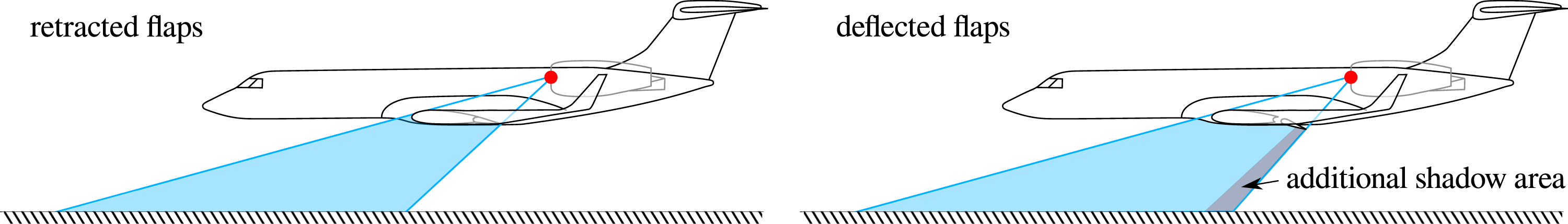
The selected setup to be simulated is designed in such a way that it can be compared to the flyover experiments with little knowledge of several details. Instead of evaluating absolute sound pressure levels (SPL), the shielding effect of the flap on the engine tones is used for comparisons. By deflecting the flaps the wing area is increased and with it the noise shadow region (see Figure 2). This setup conveys several advantages:

• The source position is known to be the engine inlet since only the engine blade passing frequencies are considered.

• In context of shielding and assuming linear acoustics the source strength can remain unknown and thus the engine details including liners are not needed.

• The directivity of the sound source is of subordinate importance since the flap is small such that most directivity effects cancel out when computing the shielding.

Figure 2.

Sketch showing the point source which replaces the engine and the expected additional shielding area due to a deflected flap.

The previous thoughts define the case to be simulated: the engine-less aircraft with and without deflected flaps. The sound is induced by a monopole source, placed at the center of the engine inlet plane. Additionally, a third case is simulated: an isolated point source without any aircraft. This allows to calculate the total airframe shielding of the source which can give more detailed insights into shielding effects.

The frequency-dependent shielding level γ(f) is defined as follows

$$\gamma \left(f\right)=SPL\left(f\right)-SP{L}_{\text{ref}}\left(f\right)$$

(1)

This means that the additional shielding of the flap γ_flap can be calculated by

$${\gamma }_{\text{flap}}\left(f\right)=SP{L}_{\text{deflected flap}}\left(f\right)-SP{L}_{\text{retracted flap}}\left(f\right)$$

(2)

In contrast, the total shielding is determined by

$${\gamma }_{\text{airframe}}\left(f\right)=SP{L}_{\text{with airframe}}\left(f\right)-SP{L}_{\text{isolated source}}\left(f\right)$$

(3)

Experimental methodology

The flyover measurements were conducted with the High Altitude and Long Range Research Aircraft (HALO) operated by the German Aerospace Center. As shown at the left hand side of Figure 3, several microphones were placed on the ground to measure the aircraft engine tones. A more detailed description of the ground board microphones can be found in the work of Pott-Pollenske et al. ⁷

Figure 3.

Left hand side: Microphones below the aircraft as used in flyover measurements. Right hand side: Transformed microphone trajectories for wind tunnel-like evaluations.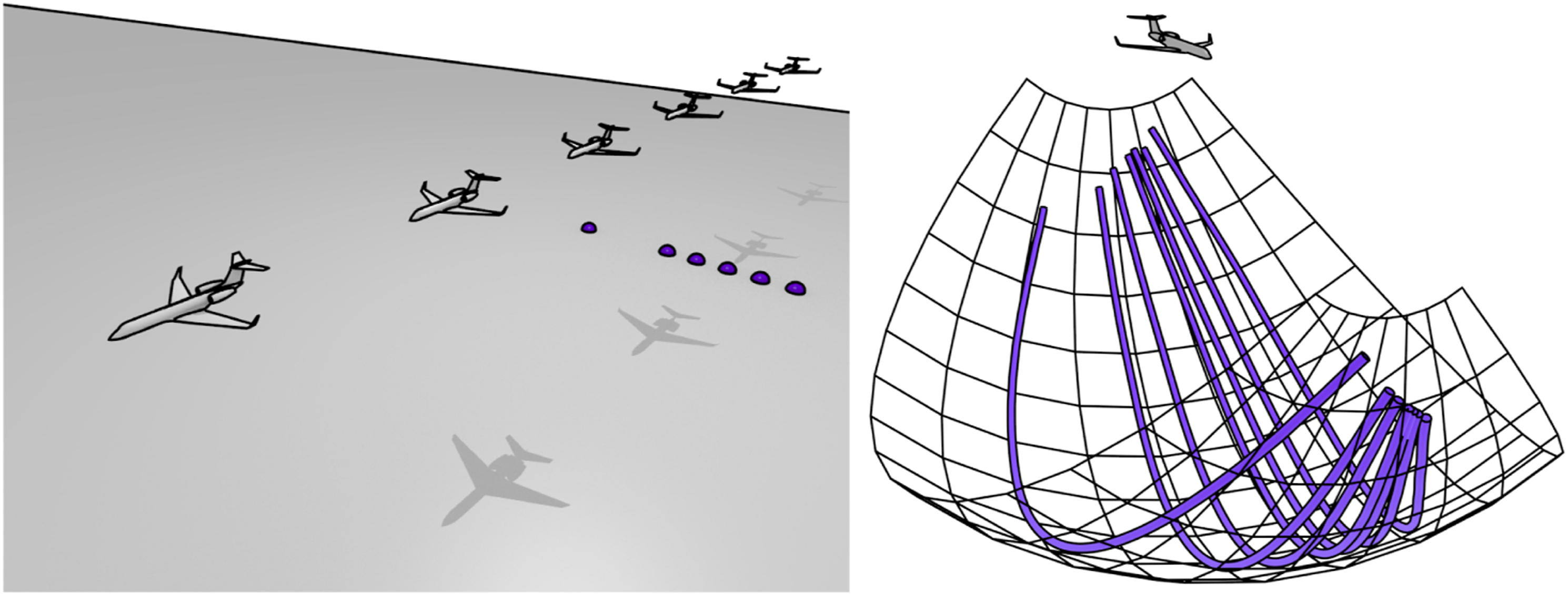

During the flyover all important parameters were recorded, such as the aircraft position relative to the microphones, angle of attack, airspeed and engine settings. This allows post-processing the data such that the frequency-wise sound pressure levels are known on spherical arcs around the aircraft center. In other words, the results are described in a wind tunnel-like setup, where the microphone positions are fixed in respect to the airplane (see Figure 3 to the right). The post-processing consists of the following steps:

1. Removing the effect of ground reflections by empirical methods based on previous measurements.

2. Removing the effect of atmospheric damping based on the relations given by Shields and Bass. ⁸

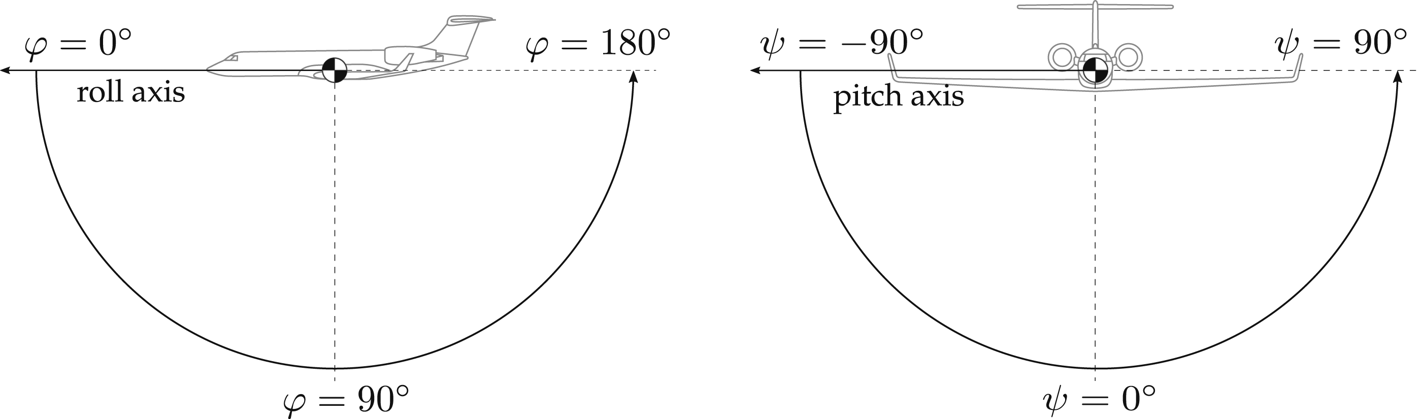
3. Correction for Doppler shift directly in time domain with a subsequent resampling of the data for equidistant time stamps.

4. Transform the data into frequency space by windowed Fast Fourier transform (FFT) for short successive time periods.

5. Map the results on a sphere with longitudinal angle φ and lateral angle ψ and a fixed distance (see Figure 4). Hereby, it is assumed that the corrected pressure amplitudes drop with the factor of $\frac{1}{r}$ where r is the distance to the aircraft.

Figure 4.

Definition of longitudinal angle φ and lateral angle ψ.

The predefined aircraft settings of the flyovers which are of importance for this paper are the rotational speed of the fan N1 = 80%, the flap position (retracted as well as deflected by 10°) and the Mach number Ma = 0.35. This implies that the 10° flap case operates at a smaller angle of attack to compensate the extra lift. The altitude over ground was about 130 m where besides of GPS tracking the exact distance was determined via an optical camera and triangulation. The flyover was repeated about 5 times for each setting in order to increase the reliability of the data. Even after removing the outliers, the trajectories show differences of up to 20 degree lateral angle as shown in Figure 5. Due to this substantial differences and in order to reduce measurement noise, the SPL was averaged ^∗ for all microphones at different lateral angles. This step comes at the cost of loosing the lateral dependency.

Figure 5.

Lateral angle ψ over longitudinal angle φ relative to the center microphone for repetitions of the same flyover scenario. Each line within each plot stands for another flyover.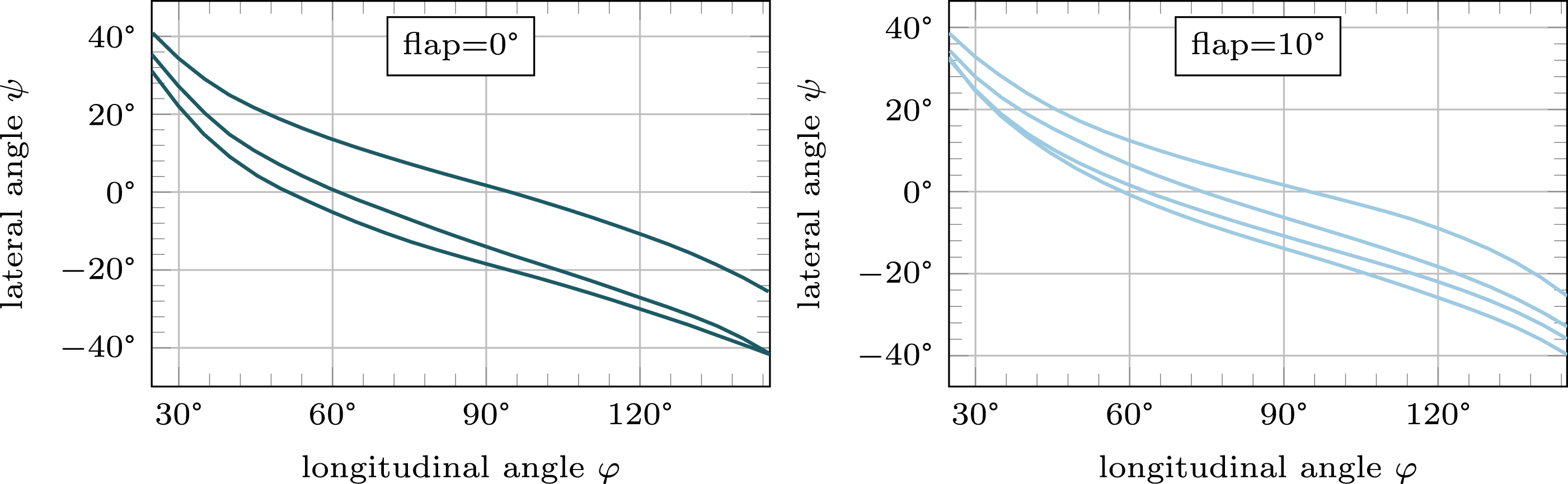

Experimental results

The left-hand side of Figure 6 shows the sound pressure levels for different frequencies over the flyover time for one microphone without any corrections applied. It prominently shows the broadband noise which increases while the aircraft approaches and decreases again when the aircraft has passed the observer. Of interest in this paper are the blade passing frequencies and their harmonics since they can uniquely be assigned to its source, the engine fan. The first blade passing frequency can be clearly seen at the beginning of the flyover amplified at an increased frequency in the forward arc due to the Doppler shift. After the aircraft passed by, this frequency drops to a smaller value which is hardly visible anymore. Applying all corrections and transformations as described during the experimental setup highlights the single tones as shown on the right-hand side of Figure 6. The de-Doppler procedure ensures that the fan tones are almost straight lines which deviate only slightly from the target frequency for the requested N1 speed.

Figure 6.

Sound pressure level during flyover for different frequencies for a single microphone. Left-hand side: FFT applied directly to raw data of a single microphone. Right-hand side: Data after removing ground reflections, atmospheric damping and Doppler shift. (legend: , ).

The present work concentrates on the fan tones found at the first two blade passing frequencies. Not relevant for the shielding effects, outside the blade passing frequencies and its harmonics, broadband noise and tones also become visible, which will not further be discussed here. Only the high amplitude at small longitudinal angles and high frequencies shall be identified as an artifact, which results from the correction of the low background noise with an extremely high prediction of atmospheric attenuation.

Even though in the flyover measurements the fan tones radiating through the intake and the bypass nozzle will contribute to the overall measurement of the fan tone, it is assumed that, at the given operating conditions, the forward radiated fan tone dominates the measured level in the angular range relevant for the shielding effect. Therefore, the simulations in the following sections will model the fan tone source with a monopole at the engine inlet plane to compare with the measured shielding effect at the blade passing frequencies.

As indicated in the previous section, before isolating the sound pressure level at the blade passing frequencies all microphone data during one flyover are averaged. This reduces variation in the measurement and makes the detection of blade passing frequencies much easier. After the precise blade passing frequency for a given longitudinal angle φ is determined, the sound pressure levels are integrated over a narrow frequency band of Δf = 100 Hz. Since the sound pressure level of a blade passing frequency is dominant over a certain frequency range, the results are not very sensitive on the choice of the integration band width. Figure 7 shows the frequency-dependent sound pressure levels averaged over all microphones as well as the instantaneous blade passing frequencies as a blue line. Both flap settings show very similar results.

Figure 7.

Extraction of sound pressure from data averaged over all microphones from one flyover. (legend: , ).

After plotting the sound pressure levels of the blade passing frequencies in Figure 8 a small effect of the flap becomes visible for the first and the second blade passing frequencies. The figure shows the data for repeated flyovers with the same settings which can give limited insights into the uncertainty of the data. Especially at longitudinal angles φ between 30° and 80° there appears a small systematic differences for different flap settings.

Figure 8.

Sound pressure levels extracted for the first and second blade passing frequency for different flap settings. Different lines within one plot with same color refer to repeated flyovers.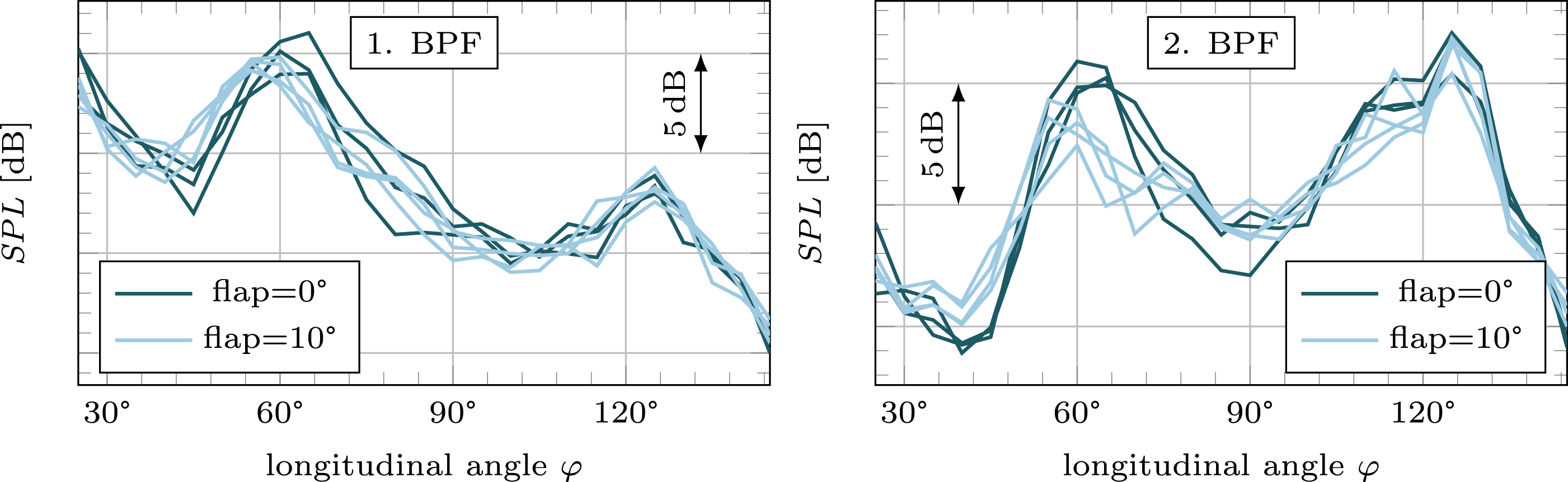

Averaging the repeated flyover data in order to further reduce scatter and then calculating the flap shielding with the help of equation (2) yields the results shown in Figure 9. It is emphasized that negative shielding levels mean less noise with deflected flaps, where positive shielding levels mean more noise after deflecting flaps. The plots show that a deflected flap (which is equivalent to an increased wing area) does not necessarily lead to less noise. Indeed, at certain longitudinal angles φ there is a positive shielding factor. There are two major possible explanations for an increase in noise: flap gaps and interference patterns. Interference patterns can be excluded since the patterns over the longitudinal angle would be substantially different for different blade passing frequencies which appears not to be the case. Most probably, the increase of noise is an effect of the flap gap which allows sound waves to bypass the wing.

Figure 9.

Flap shielding γ_flap(f) = SPL_{deflected flap}(f) − SPL_{retracted flap}(f), based on the averaged data of all microphones and all repeated flyovers including the error bars showing the standard deviation between different flyovers.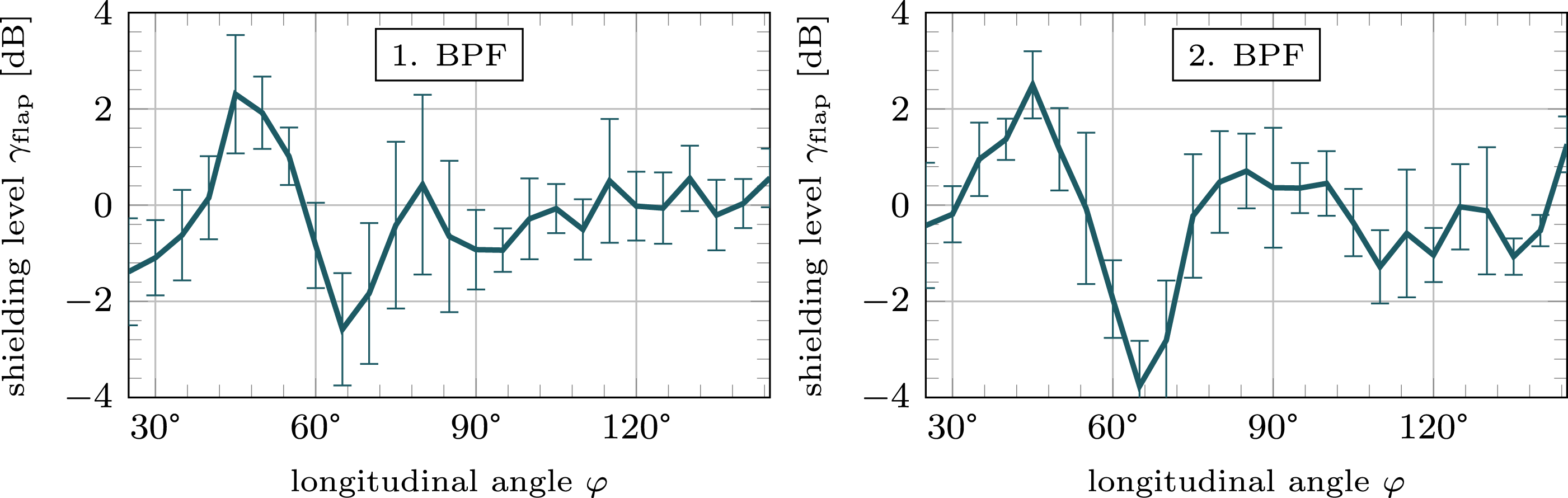

The plots also show the standard deviation

$$\sigma \left({\gamma }_{\text{flap}}\right)=\frac{10}{\mathrm{l}\mathrm{n}10}\cdot \sqrt{\left(\frac{{\sigma }^2\left(p_{\text{retracted flap}}^{\prime 2}\right)}{{\overline{p_{\text{retracted flap}}^{\prime 2}}}^2}+\frac{{\sigma }^2\left(p_{\text{deflected flap}}^{\prime 2}\right)}{{\overline{p_{\text{deflected flap}}^{\prime 2}}}^2}\right)}$$

(4)

where the overline marks the ensemble average over different flyovers and σ is the standard deviation. The error formula is derived based on the definition of the sound pressure level

$$SPL=10{\log }_{10}\left(\frac{p^{\prime 2}}{p_{\text{ref}}^2}\right).$$

(5)

Due to the very limited number of flyovers the error is rather large in the range of about ± 1 dB. Still the trends show a very clear picture of the flap shielding effect.

Numerical methods and simulation setup

During the case setup it was already outlined that the simulations do not use the sound coming from the real engine but replace it with a monopole source. The geometry of the aircraft and the monopole source is sketched in Figure 10. The visualization emphasizes that only at the position of the right engine the source is applied. The sound emitted from the left engine is added during a post-processing step by assuming a symmetric aircraft and incoherent sources.

Figure 10.

Visualization of source as a red dot.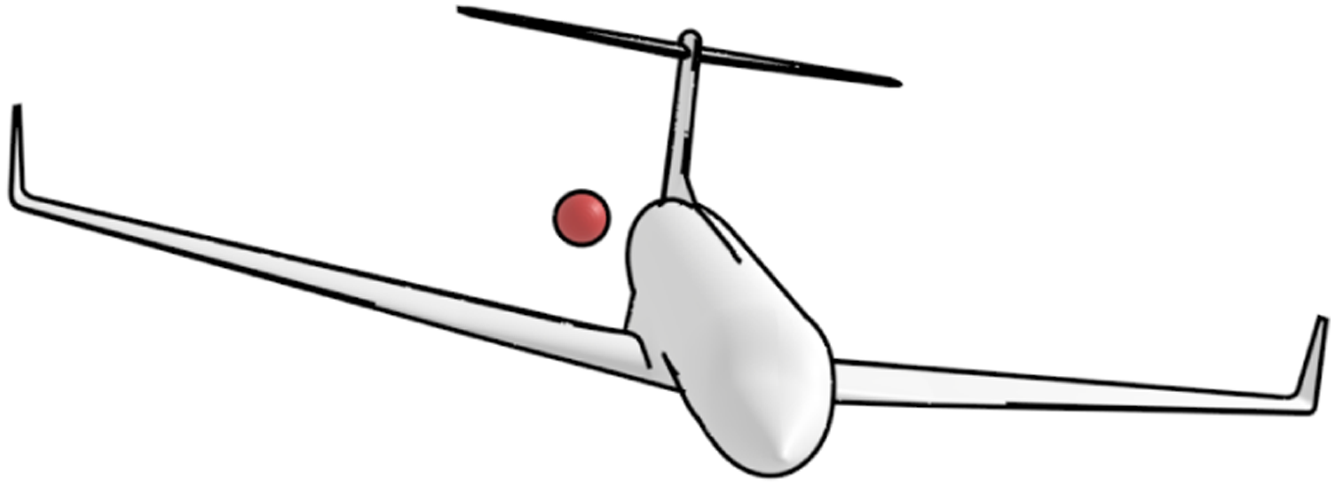

For reproducing the microphone positions of the experiments (recall Figure 3) one representative trajectory for the flyovers was chosen. A symmetric setup is enforced by duplicating and mirroring the locations at the aircraft’s symmetry plane (Figure 11 to the left). Besides the microphone positions of the flyover experiment, many additional observer points are added on a plane 51m below the aircraft as depicted in Figure 11 to the right. This allows creating a footprint of shielding levels.

Figure 11.

Left hand side: Microphone lines below the aircraft as used in flyover measurements plus microphones mirrored at the aircraft symmetry plane. Right hand side: Additional evaluation area for creating a shielding level footprint.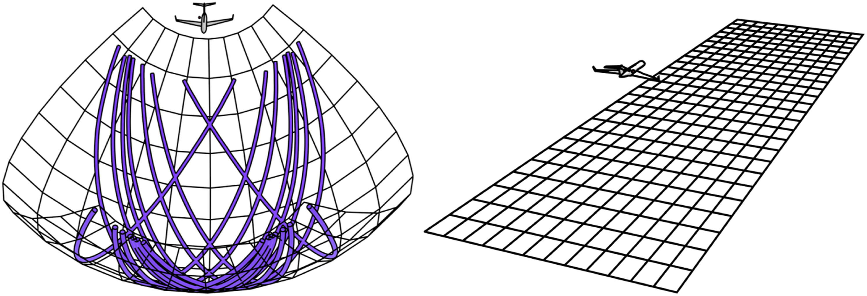

The setup was computed with two different methods: A boundary element method and a volume-resolved discontinuous Galerkin method. The boundary element method ⁹ is solving the Helmholtz equation. Using Taylor transformation it can take a spatially uniform mean flow into account as long as the Mach number is moderate. Only the application of a fast multipole acceleration technique makes it possible to solve the equation with a reasonable amount of computational resources. The boundary element surface mesh was created to resolve one wavelength with at least six elements. Since the Helmholtz equation is defined in frequency domain the shielding is computed for each examined frequency separately. Experience tells that the Mach number of about Ma = 0.35 is already at the limit of what is allowed meaning that the errors made by Taylor transformation are already starting to grow. Also the flow close to the aircraft considerably deviates from the constant value. However, comparisons with experiments will show that the method is still accurate. Additionally, for low frequencies the results can be checked with the help of volume-resolved methods.

Such a volume-resolved method is the second numerical strategy to solve the problem, a fourth order discontinuous Galerkin method. ¹⁰ It solves the acoustic perturbation equations ¹¹ which avoid any hydrodynamic instabilities that can occur e.g. in the wake of the wing. The equations are solved in time domain on top of a steady mean flow which can either be a uniform value as taken for the boundary element method or a fully featured Reynolds averaged Navier-Stokes (RANS) solution. Using a quadrature free approach with high order tetrahedrons makes the method very efficient. ¹² Still, the number of cells would be far too high for propagating down to the microphone positions. This problem is counteracted by solving only in the near-field of the aircraft and then using a Ffowcs-Williams-Hawkings extrapolation to bridge the large distance. The region resolved by the discontinuous Galerkin method is sketched in Figure 12. Similar to the boundary element method, the Ffowcs-Williams-Hawkings extrapolation only considers a spatially constant Mach number, but since it is only applied after the waves left the immediate aircraft near-field, the results can be expected to be very accurate. The volume-resolved mesh is designed to resolve the expected wavelengths with about two high order cells. No special care is taken to resolve boundary layers of the RANS solution, meaning that especially at the wing leading edge the boundary layer is strongly under-resolved. The expected effect of this simplification is small.

Figure 12.

Sketch of volume resolved region inside the colored region, the Ffowcs-Williams-Hawkings surface around the colored region and the footprint area.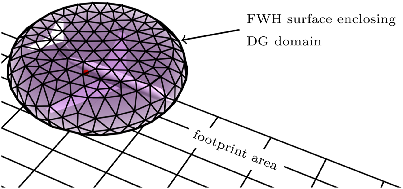

It should be mentioned that for obtaining the RANS mean flow itself, the boundary layers are fully resolved where the first cell thickness above a wall fulfills the typical 1y condition. The turbulence model is a Spalart-Allmaras one-equation model and it is solved for steady state. For using the mean flow on the discontinuous Galerkin mesh, mesh-to-mesh interpolation is used.

Comparing the boundary element solution to flyover data

The boundary element methods is compared to the flyover experiments by solving for the first two blade passing frequencies with retracted and deflected flaps and using the results to calculate the flap shielding γ_flap. The comparison between experimental and numerical data is shown in Figure 13. The lines of experiment and simulation have very similar shapes showing an increase of noise of about 2 dB at small longitudinal angles φ and a decrease of similar magnitude at slightly larger angles. Apparently, the boundary element simulations are capable of predicting the very small changes of the noise pattern when deflecting the flap. However, the line of the simulation results is clearly shifted by an approximate angle of Δφ ≈ 20°.

Figure 13.

Comparison of boundary element simulations (sim.) against the flyover measurements (exp.) for the first two blade passing frequencies.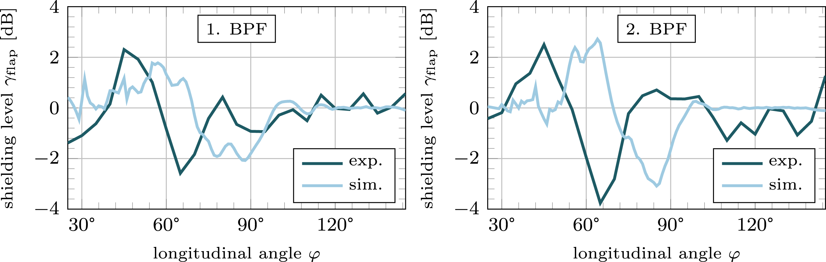

One explanation for the shift of the curves is that the source is not correctly positioned. All simulations are simply using the straightforward position of the engine front plane. However, replacing the fan by a monopole source is not exact, but rather the fan noise would have to be described by a distributed source. In order to avoid increasing the complexity by simulating a distributed source, the sensitivity of a monopole shift on the result is investigated. This shift can be understood as a better projection of the distributed source onto a monopole. Figure 14 sketches a modified source position which is moved downstream by 0.5 m. The boundary elements simulations are repeated and the results plotted in Figure 15.

Figure 14.

Sketch of shifted point source for modified numerical setup.

Figure 15.

Comparison of boundary element simulations (sim.) against the flyover measurements (exp.) for the first two blade passing frequencies after shifting the source position backwards.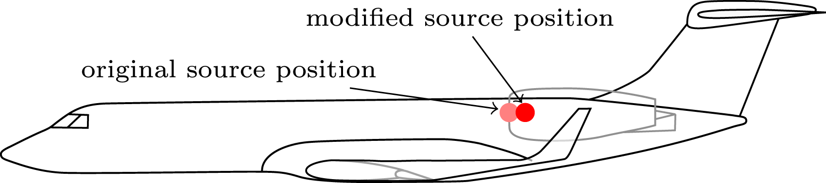

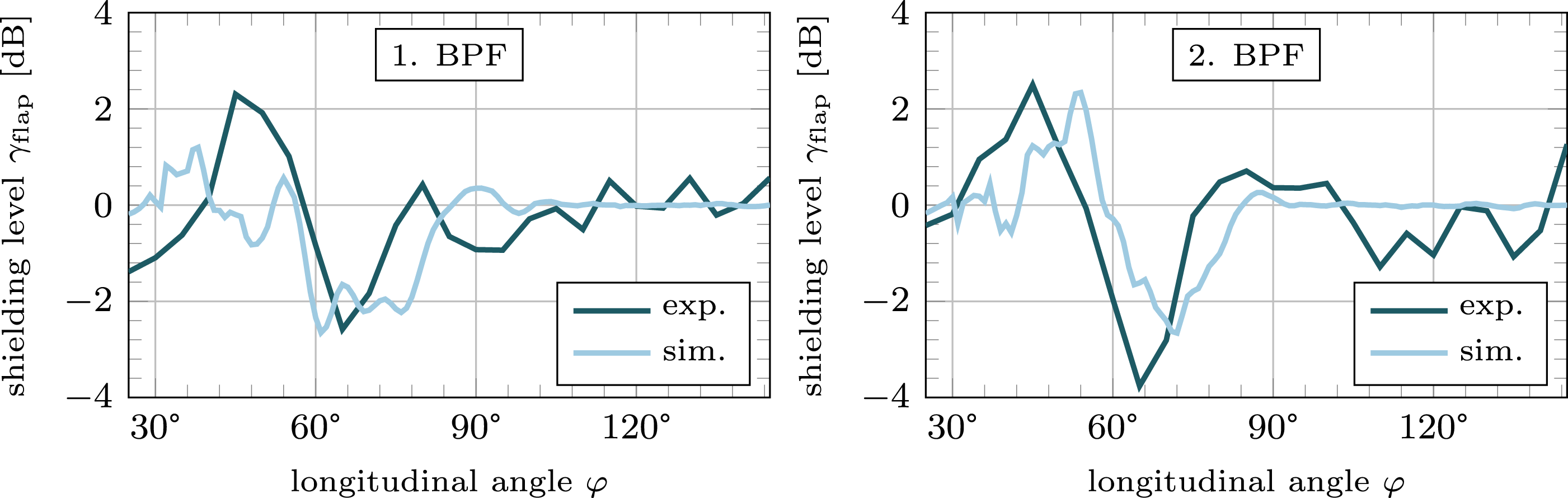
Indeed, the simulation result is shifted upstream, leading to a much better match with the flyover measurements. However, the improvement by shifting the source comes at the cost that for the 1. BPF case the 2 dB peak at longitudinal angles around φ = 45° is not captured very well anymore. Obviously, the correct description of the source is very critical to reproduce the results. This should not curtail the fact, that the very small effect of flap shielding is captured nicely despite the simplifications made.

The left hand side of Figure 16 gives a bit more insight by visualizing flap shielding γ_flap for the first blade passing frequency as a footprint 51m below the aircraft. One can clearly see the decrease of noise at longitudinal angles of φ ∼ 80° where the blue color is dominant. Upstream of this region there are strong interference patterns. There, the red color is more dominant in agreement with the previous comparisons with experiments. The figure also shows the significant shift of the flap shielding region to smaller longitudinal angles φ for a downstream shift of the source.

Figure 16.

Flap shielding γ_flap (left hand side) and total airframe shielding γ_airframe with deflected flap (right hand side) as footprint for a source at the engine front plane and a source shifted downstream by 0.5 m. The shown frequency corresponds to the first blade passing frequency.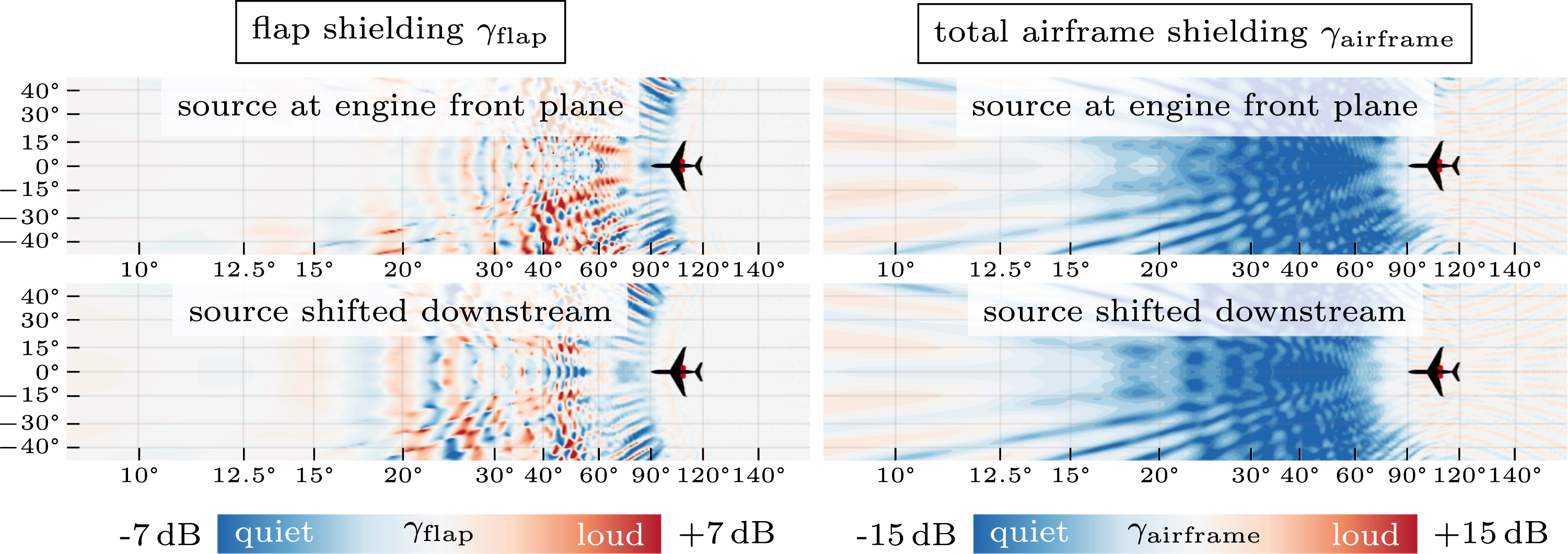

On the right hand side of Figure 16, the total airframe shielding γ_airframe is shown. Obviously, the shielding levels resulting from wing and fuselage are much higher here compared to the flap shielding γ_flap which is only a very small part of the total shielding. One can see that at longitudinal angles φ between 20° and 90° the first blade passing frequency is attenuated by 15 dB and more, where there is hardly an increase of noise at other angles. This emphasizes to potential of shielding for reducing the noise immission on the ground, however this result must be taken with care. In order to get realistic results for the total airframe shielding the radiation characteristics of the source must be taken into account.

Comparing the boundary element method to volume-resolved results at a constant mean flow

The comparison with the flyover data already presents the good prediction capabilities of the boundary element method. This indicates that the shortcomings of the boundary element method (constant mean flow, small Mach numbers) do not play a major role at Ma = 0.35. Still, it is interesting to investigate the effect of the mean flow in more detail. In order to gain more insight, the boundary element results are compared to volume-resolved discontinuous Galerkin results. Due to the very high computational cost of the volume-resolved method (see Table 1) the maximum affordable frequency is limited to about 1 kHz. This is well below the first blade passing frequency of the flyover measurements, such that a direct comparison is not possible. But the results allow additional insight into the mean flow effects at lower frequencies and also serve as an additional reference for boundary element method. In order to better isolate the different mean flow effects, two different comparisons are made:

1. Comparing the boundary element to volume-resolved results obtained with a constant mean flow.

2. Comparing volume-resolved results with constant mean flow against results with RANS mean flow.

Table 1.

Approximate problem sizes for the investigated solvers at two frequencies.

		BEM	DG
f = 1 kHz	Number of elements	600 000	80 000 000
—	Cost in core hours	$\approx 50$	$\approx 230\hspace{0.17em}000$
f = 6 kHz	Number of elements	25 000 000	-
—	Cost in core hours	$\approx 10\hspace{0.17em}000$	-

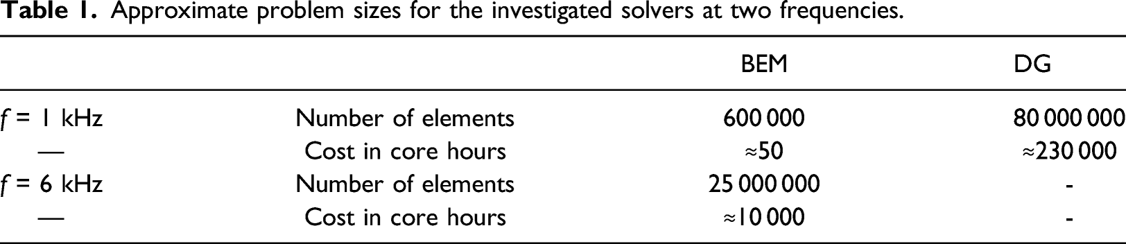
The current section discusses the first point.

Figure 17 compares the flap shielding γ_flap of the boundary element method (BEM) with the volume-resolved discontinuous Galerkin (DG) method. The evaluation is conducted in accordance with the previous sections using the microphone position from the flyover experiments and averaging the results. As already mentioned, for the current section the results of the DG method are computed with a spatially constant mean flow. So as long as the Taylor transformation errors of the boundary element method are small the results should match very well. Indeed, the two very different methods show very similar results at the two compared frequencies. But one can see that especially at very low frequency (f = 198 Hz) the interference patterns are less prominent for the boundary element method. Comparing with more frequencies in-between f = 198 Hz and f = 900 Hz not depicted in this paper indicates that the error tends to get smaller with increasing frequencies, however interference patterns can be very sensitive to parameter changes so that no final statement can be made.

Figure 17.

Comparison of flap shielding between boundary element method results and volume resolved DG results with spatially constant mean flow for two different frequencies.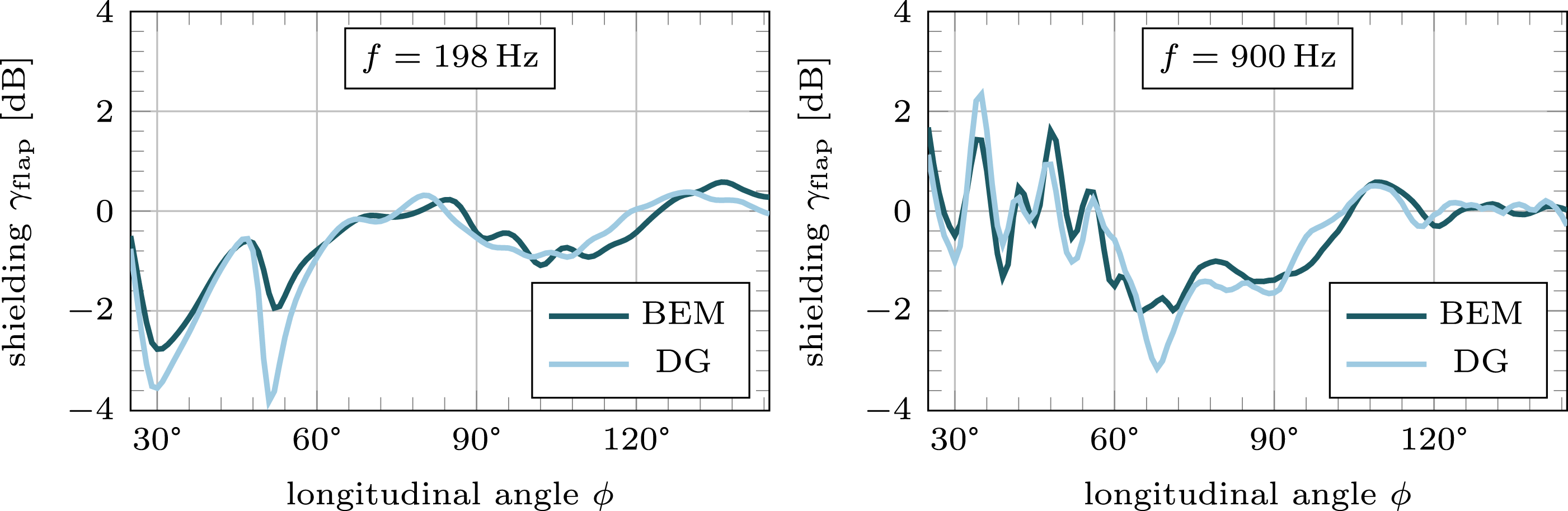

In total, the boundary element method predicts the trends of flap shielding effects very well. Yet the effects of the spatially varying mean flow field are not yet quantified. Especially the boundary layers are known to lead to refraction of sound waves. ¹³ To gain more insight into such effects, the volume-resolved DG method was rerun with a realistic RANS mean flow.

Mean flow effects at low frequencies

As mentioned previously, the volume-resolved discontinuous Galerkin method is a hybrid method which solves the acoustic perturbation equations on top of a mean flow field as e.g. obtained by a RANS simulation. The present sections compares a more realistic RANS mean flow with a constant mean flow both obtained with the same discontinuous Galerkin solver. Note that the underlying aircraft geometry for obtaining the mean flow results was just approximate and several aircraft details (e.g. engine, flap tracks) are missing, but the basic flow topology with the boundary layers match well enough to get a good estimate of how the mean flow affects the sound waves.

Figure 18 compares the flap shielding γ_flap at two different frequencies for a constant mean flow and a RANS mean flow. The footprints indicate that for the two rather low frequencies there is not such a significant shielding by the flap as it was observed for higher frequencies (recall Figure 16). The dominance of the interference patterns hides most of the shielding effects. Especially, for very low frequencies as e.g. f = 198 Hz it is hard to find similarities between the constant mean flow and the RANS mean flow. Here, the wavelength of about 1.5 m is much larger than the increase of the wing chord length by deflecting the flap (∼ 0.5 m). At such large wavelengths the differences in the interference patterns due to a modified mean flow appear to dominate over the effect of deflecting a flap. The situation is very different for the frequency of 900 Hz. Here, the footprint patterns for the different mean flows are very similar. Obviously, for shorter wavelengths, the mean flow has not such a big influence on the flap shielding anymore.

Figure 18.

Comparison of flap shielding γ_flap footprints for a constant mean flow (Ma = 0.35) and for a RANS mean flow.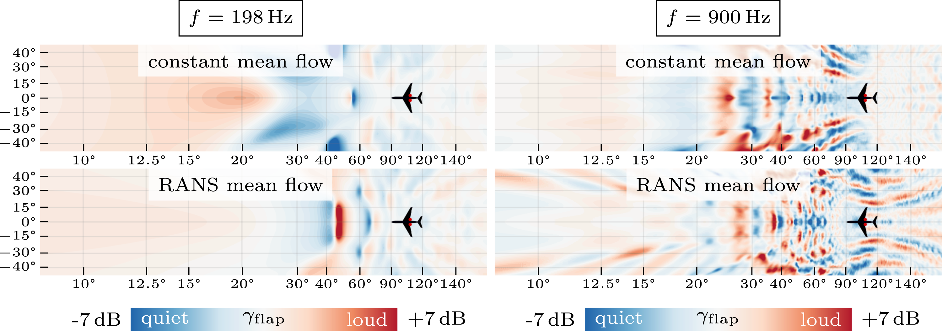

The described effects are shown in a more quantitative manner in Figure 19, showing the averaged flap shielding γ_flap at the measurement microphones. Especially at the strongly shielded regions of longitudinal angles φ between 30° and 80°, the interference patterns strongly differ as long as very low frequencies (198 Hz) are considered. For higher frequencies (900 Hz) the trends are much more similar for the different mean flows, but with local discrepancies remaining (most prominently at 70°). It is expected, that at the blade passing frequencies which are way higher than 900 Hz, the comparison would match even better. This is at least an indication, that the boundary element method (which uses a constant mean flow) can indeed be used for high quality comparisons when comparing the results to flyover experiments.

Figure 19.

Mean flow effect on flap shielding for a constant mean flow and a RANS mean flow.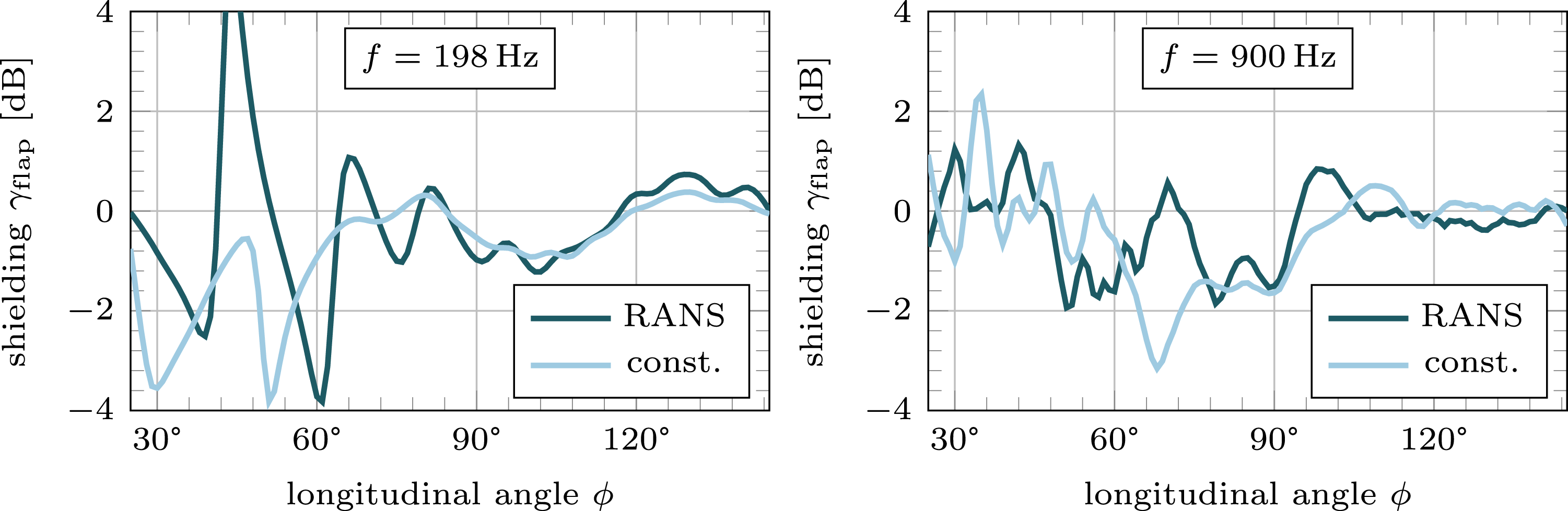

It is interesting to investigate the flap shielding results further in context of the total airframe shielding γ_airframe. A footprint is shown in Figure 20. The f = 198 Hz case shows that when switching from a constant to a RANS mean flow the interference pattern in front of the aircraft is substantially transformed. The blue peak for a constant mean flow at a longitudinal angle of about φ = 50° redistributes into several peaks around its original position. However, the overall shielding distribution it is still very similar for both mean flows. This is particularly true when comparing the strong shielding part directly upstream of the aircraft. Apparently, total shielding predictions with a constant mean flow capture the major effects even for low frequencies but not the exact interference patterns. In contrast, details like flap shielding cannot be reliably predicted at these low frequencies as long as the exact mean flow is not considered. When the frequencies increase, there are still significant differences between the two different mean flows, however, the interference patterns look more similar meaning that flap shielding effects can be much easier predicted by just using a constant mean flow.

Figure 20.

Comparison of total shielding level γ_airframe footprints for a constant mean flow (Ma = 0.35) and for a RANS mean flow in case of deflected flaps.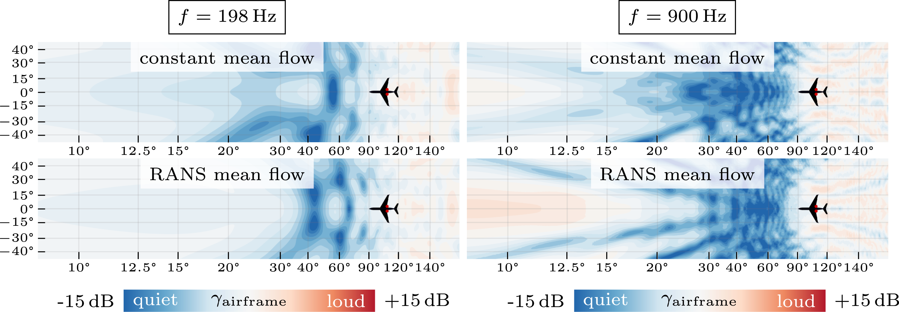

Up to now, the discussion mainly referred to changing interference patterns when using different mean flows. Besides of interference effects there can also be systematic effects. Such effects would systematically deflect the sound waves in a way that not only the pattern changes, but a substantially different amount of sound energy will reach the ground. A prominent candidate for systematic effects is refraction in boundary layers as e.g. described by Delfs ¹⁴ and sketched in Figure 21. In case of flap shielding such systematic mean flow effects are expected to be very small, but for the total airframe shielding the situation is not as clear. In theory, the fuselage would refract the upstream radiating sound away from the center-line and the wings would refract the sound away from the ground. When looking at Figure 20, no such effect can be observed, but the contrary seems to be the case: There is e.g. a slight increase of noise around the center-line at longitudinal angles smaller 15° for the RANS mean flow at f = 900 Hz. Obviously, systematic mean flow effects do not play a major role when it comes to shielding, at least not for the investigated frequencies. This is in accordance with the results presented by Delfs et al. ¹³ for a 2D study.

Figure 21.

Sketch showing sound refracting in a boundary layer.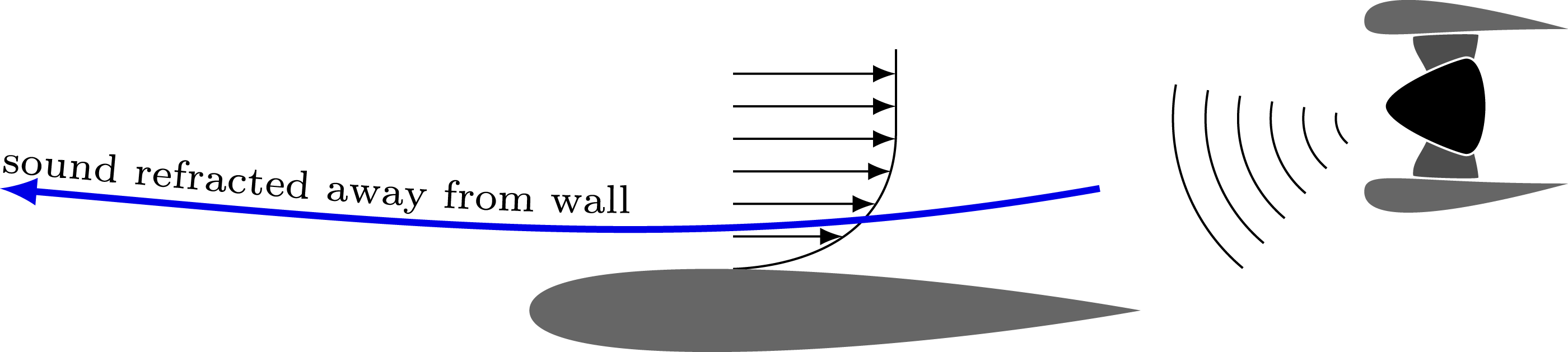

For sake of completeness it should be mentioned that the computational grid for the acoustic simulations is rather coarse compared to the boundary layer thickness. The wing boundary layers thickness does not much exceed 0.1 m which is in the same order as the edge length of a high order cell (the solution in such a cell is described by a third order polynomial). But this should be enough to at least capture the trends.

Conclusion

The presented work compares experimental flyover data to numerical predictions by evaluating engine tone shielding of a deflected flap. Also an insight into the effects of mean flow around the aircraft on the noise immission on the ground is given.

By evaluating the increased noise shielding when deflecting a flap, no detailed information about the engine is needed but a monopole with a uniform radiation pattern and unit source strength is used. It is shown, that a boundary element method can predict the right trends and orders of magnitude. However, it becomes also visible, that the strong simplification of using a monopole introduces new uncertainties as finding the correct equivalent position to mimic the behavior of the engine in an accurate way. This means that for new aircraft designs the boundary element method can predict good trends of airframe shielding effects, but if very accurate data is needed it will be indispensable to simulate a more realistic source.

Since the boundary element can only take a spatially uniform mean flow into account, the mean flow effects are investigated subsequently by a second method, a volume-resolved discontinuous Galerkin method. Since this method is computationally very demanding dependent on the resolved frequency, no direct comparisons to the flyover experiments are possible. Instead, the mean flow effects are investigated at frequencies significantly below the first blade passing. While for very low frequencies, the flap shielding is very dependent on the mean flow, the discrepancies appear to decrease with increasing frequencies. By further evaluating the total airframe shielding, it is shown that the mean flow mainly changes the pattern of interference patterns, but a systematic reduction or increase of noise at the ground cannot clearly be detected.

In conclusion it is shown that a boundary element method can well predict shielding effects on engine tones even if only a small detail like a deflected flap is examined. The fact that boundary element methods can not take a realistic mean into account flows seems not to play a major role for the results especially as long as the frequencies are high enough. For lower frequencies the behavior changes and the mean flow effects more and more overshadow details like flap shielding. If the focus is not on the details but more on the overall effects like the total airframe shielding, no significant increase or decrease of sound immission on the ground can be observed.