
Abstract
An experimental study has been carried out in a laboratory flume to characterize the turbulence structure and turbulence anisotropy in the boundary layer over smooth and rough side walls for both current alone and wave-current combined flow situations. The rough side wall of the flume comprises a train of circular ribs (diameter, k) attached vertically maintaining uniform spacing p along the streamwise direction. The experiments are performed for smooth surface and rough (ribbed) surfaces with p/k = 2, 3, and 4 to reproduce different cases of d-type rib roughness. The effect of wave-current interaction has been investigated by superposing waves of two different frequencies. Time series data of three velocity components are obtained using Acoustic Doppler Velocimeter. At the near wall region, roughness with higher p/k value enhances the level of turbulent intensity and Reynolds stress significantly. In a channel with smooth side wall, the wave-current combined flow produces lesser turbulence intensity than the current alone flow near the wall. However, for a ribbed wall case, the effect is completely opposite that is, wave-current interacting flow induces higher intensities compared to the reference current alone flow. Substantial decline in the turbulent length scales at the near wall region are observed for ribbed walls, which reveals the strong effect of roughness elements on the turbulent structure. Superposition of wave reduces the length scales even more for both smooth and rough wall cases. As the spacing between two ribs (p/k ratio) increases, the energy dissipation rate increases. The analysis of anisotropy invariant map demonstrates a reduction of anisotropy in the vicinity of ribbed wall compared to that for a smooth wall. For wave-current combined flow, the anisotropy invariant data of Reynolds stress tensor varies dramatically within the boundary of map, reflecting significant changes in the state of turbulence.
Keywords
Introduction
Many fluid engineering systems deal with turbulent flows induced by uneven surfaces. The surface roughness essentially increases both the flow resistance and the rate of momentum transfer. To modulate the turbulence structure in the flow, surfaces are often artificially roughened. Since Nikuradse’s 1 seminal work on flow through rough pipes, turbulent flow over uneven surfaces has been investigated extensively due to its technological importance. Studies on the turbulence characteristics of coexisting wave and current flow has been scarce despite the fact that such wave-imposed current flows are of great importance for the understanding of flow resistance and sediment entrainment in the coastal environments. The combination of wave and current flows govern many physical processes of interest to the engineers and researchers working in coastal environments. Grant and Madsen 2 carried out a theoretical analysis of wave-current combined flow over a rough surface boundary and reported an increase in apparent bed roughness and shear stress when waves were superimposed on the current. Later Kemp and Simons 3 performed an experimental study in a laboratory channel for wave-current combined flow over smooth and rough boundaries and reported a considerable increase in bed shear stress for rough boundary when waves are superimposed on the current flow. Moreover, Kemp and Simons 4 documented a significant reduction in sidewall boundary layer thickness and mean motion in the vicinity of the sidewall for wave-current combined flow. Further the results indicated that a redistribution of flow occurs across the channel for such wave superimposed flows. Thus, the flow structure of wave current combined flows has been a subject of great interest to numerous academicians and researchers. Yu et al. 5 conducted a study to resolve the turbulent scales for oscillatory boundary layer over rough wall covered with two-dimensional roughness elements. They reported that the dynamics depends on both the shape and size of the roughness elements and their relative positions that is, pitch-to-height ratio. Yu et al. 5 also examined the anisotropy of turbulence through anisotropy invariant map (AIM) analysis for rough wall oscillatory boundary layer and found that turbulence becomes more isotropic when moves toward the outer boundary layer.
In this paper the turbulence characteristics are presented for wave-current combined flow over d-type rib roughness on the side wall of a channel based on laboratory flume experiments. One of the important parameters for the characterization of turbulence is the turbulent length scales which are based on measured velocity time series. The invariant analysis of Reynolds stress tensor 6 is also presented in the present study, to extract information about the anisotropy of large-scale motion. 7 In view of applying turbulence closure models in RANS based CFD simulations, it is of great importance to have some prior knowledge of expected anisotropy of the flow field under exploration. Shafi and Antonia 8 suggested that the knowledge of this anisotropy is of much help in the determination of the sensitivity of turbulence structure to different boundary conditions. Particular interest was paid to the sidewall near boundary turbulent flow within the roughness sublayer, with the concept of wall similarity hypothesis that turbulent motion outside the roughness sublayer are almost independent of the wall boundary condition.9–11 Krogstad and Antonia 12 indicated the differences of large-scale structure between the smooth and rough walls in view of anisotropy of Reynolds stress between the smooth and rough wall flows.
Various roughness elements such as sand grains, gravels, spheres, cubes, wire mesh and two-dimensional ribs (circular, square) attached to the boundary wall surfaces were investigated in the past to model surface roughness. Understanding the flow characteristics over these roughness elements received a lot of attention due to its application in numerous areas of engineering and environmental sciences. According to Perry et al., 13 the rib roughness is classified as d-type and k-type based on the pitch-to-roughness height ratio (p/k): p/k < 5 considered as d-type, p/k > 5 considered as k-type and p/k = 5 as intermediate roughness. Ribs roughness are employed in many engineering applications to augment heat transfer rates and also often used to study the effects of surface roughness on momentum transport. 14 Understanding the impact of roughness on the transport and mixing of contaminants such as wastewater and oil discharged into river systems by industries or natural disasters is critical from an environmental point of view. 15 To improve engineering design practice, a thorough understanding of roughness effects on mean motion and turbulence characteristics is required. Turbulent flow over uneven surfaces are far more complicated than flow over flat ones. The interaction of the flow with the protrusion of the roughness elements attached to the boundary wall, both in terms of mean velocity and turbulent quantities is complex. Further when the turbulence generated by the wave-current combined flow interacts with the turbulence caused by roughness elements, the flow becomes more complex.
Numerous experimental and numerical investigations have facilitated the acquisition of information on the complex behavior of wave-current interaction flow over smooth surface and various rough surface boundaries. Several studies on the interaction of wave and current flow over smooth boundary have been carried out experimentally3,16–19 and numerically5,20–22 to examine the mean velocities, turbulence intensities and Reynolds stresses. Further equal importance over rough boundary has been given from past. Mostly the studies were focused on the bottom roughness such as ripple bed,23–25 series of square rib elements spanning the width of the channel bed surface, 26 5 mm high triangular wooden strips stuck on the bed across the channel width with the spacing between two consecutive strips about 18 mm which corresponded to p/k < 5 known as d-type roughness. 3 Similarly, Barman et al. 27 used chain of hemispherical ribs with p/k = 2, 4, and 8 as the bottom roughness. Kemp and Simons 3 showed that the near-bed velocity decreased over a rough surface, whereas the near-bed turbulence intensity increased in the presence of waves. Kemp and Simons 4 investigated the sidewall boundary layer thickness in addition to the bottom boundary layer and reported that sidewall boundary layer thickness dramatically reduced by approximately 4 times that of current alone flow for the wave current combined flow. The overall result of the study of Kemp and Simons3,4 indicated a redistribution of flow across the channel for wave current combined flow. It has been an important subject to researchers with relevance to the pipe flow, canal and river flow and river bank erosion process. However, vertical bank or sidewall for canals and rivers comprises of different roughness scales that introduce additional turbulence scales at the bottom boundary layer turbulence. Hansda and Debnath 28 carried out an experimental study to look into the distribution of mean velocity, turbulence intensity, Reynolds shear stress and streamwise integral length scales over a sand-grain rough and granule rough sidewall boundary under the wave-against current flow. Investigation of turbulence structures and eddy scales close to the sand-grain and granule rough sidewall surfaces due to interaction with wave-current combined flows were presented in Hansda et al. 29 By varying the submerged vegetation on a vertical wall, velocity and the turbulence structure was studied for waves, current alone and wave-current combined flow by Chen et al. 30 Throughout the water column, the obtained turbulent kinetic energy was relatively larger in magnitude for wave-current combined flow than the current alone flow. The riverbanks may have varying combination of submerged and non-submerged vegetation. 31 These vegetations attribute to varying degrees of roughness in the bank wall 32 and the roughness influenced the turbulent kinetic energy 33 Further Czarnomski et al. 34 reported that the turbulence intensities near the bank wall influenced by the bank vegetation roughness. Yu et al. 35 analyzed the boundary layer dynamics and bottom friction in wave-current combined flows over large roughness elements and showed that waves enhance the drag force on the current flow and time averaged Reynolds stress at the top of the roughness.
In the present paper, flow and turbulence structure under the influence of d-type rib roughness (p/k < 5) attached to the side wall of the channel are extensively investigated for both current alone flow and wave-current combined flow. By varying the spacing (p) between successive circular ribs, the equivalent sand-grain roughness, ks, 1 has been altered, and thus, the turbulence characteristics of the rough boundary layer has been amended without changing the roughness height, k. Cui et al. 36 showed that within the cavity of two successive rib elements, velocity, Reynolds stress and turbulent kinetic energy are very small, and each of these variables reaches a maximum near the rib height. Traditionally, most studies in this field portray the distribution of pertinent parameters such as mean velocity, turbulent intensity, Reynolds stress, higher order moments, eddy viscosity, mixing length, turbulent kinetic energy over both d-type and k-type rib roughness for turbulent current-only flow. Thus, there is indeed a dearth of investigation for wave-current interacting flow although it appears in a wide spectrum of real-life applications (e.g. environmental flows). In view of that, this paper undertakes a details study of turbulent characteristics of the side wall boundary layer over d-type rib roughness attached to the sidewall of the channel with a special emphasis on the wave-current combined flow. Here, two different wave frequencies (f = 0.4 and 0.8 Hz) are superimposed on the main flow. In order to explore the effects of the variation of p/k and wave-current interaction on the turbulent length scales (largest integral length scale, intermediate Taylor scale and smallest Kolmogorov scale) and anisotropy of Reynolds stress, time series data of velocity components are obtained using Acoustic Doppler Velocimeter (ADV). Turbulence characterization is carried out through the estimation of turbulent length scales in which both the largest scales comprising the large-scale energy production and the smallest scales comprising the energy of dissipative scales are examined. One of the most interesting findings of the present study is that the superposition of wave reduces the integral length scale (∼ largest eddy size) for both smooth and rough wall cases. With an increased wave frequency (f = 0.8 Hz case) the largest eddy size is reduced even further. The estimates of smallest or Kolmogorov length scale demonstrate similar effects of wall roughness and wave. The role of d-type roughness on energy dissipation rate is thoroughly investigated, too. The anisotropy invariant map (AIM) of Reynolds stress tensor is carefully computed as understanding the anisotropic structure of the turbulent flow field is of considerable interest for RANS based computational analysis. AIMs of current alone flow and wave-current combined flow for various p/k wall roughness (d-type) are compared with the respective AIM data obtained for smooth side wall cases. Results show intriguing diversity in the state of turbulence, reflecting intricate interaction of d-type wall roughness and superimposed surface waves.
Experimental details
Water flume and experiment setup
Experiments were performed in an 18 -m-long open channel flume situated at the fluid mechanics and hydraulics laboratory, Indian Institute of Engineering Science and Technology (IIEST), Shibpur, India. The width and depth of the channel were 0.6 and 0.9 m, respectively. The flume wall at the test region was made of transparent Perspex to facilitate proper visualization of the flow. The “rough side wall” was fabricated by attaching a train of circular wooden rods (ribs) to it, as shown in Figure 1(b). The rib diameter (k), which essentially represents the roughness height, was kept constant (k = 15 mm) during the investigation. The roughness characteristics of the side wall was altered by varying the spacing between two successive ribs as p = 30, 45, and 60 mm which yielded pitch-to-roughness height ratio, p/k = 2, 3, and 4, respectively (see Figure 1(c)). All three p/k values considered here conform to the classical definition of d-type roughness. 13
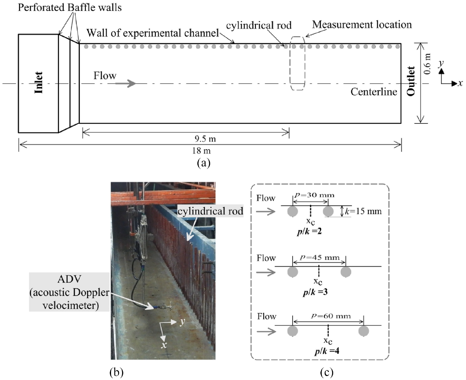
(a) Schematic of open channel (plan view) showing rough side wall, measurement location and coordinate system (not to scale), (b) photograph of rough side wall and ADV, and (c) sketch of p/k = 2, 3, and 4 and data collection position (xc).
To achieve the d-type rough side wall, the ribs were glued onto the side wall, according to the chosen spacing (p) value, vertically that spanned the height and entire length of the channel wall (Figure 1(b)). Uniform flow was maintained by using series of wire mesh perforated baffle walls at entrance of the channel. The mean (depth average) velocity (U) of current alone (CA) flow and water depth (h) were maintained as 34.6 cm/s and 20 cm for all experimental runs. Thus, in the present experimental program, all the experimental runs were carried out for the Reynolds number
For the purpose of velocity data collection in the wave current combined flow the 16 MHz micro acoustic Doppler velocimeter (ADV) was used in the experiment. The ADV was mounted in a carriage which allowed traversing in the x, y and z direction corresponds to streamwise, transverse and vertical direction respectively of the flume channel (see Figure 1(b)). The ADV system was equipped with a transmitter and three receivers. The intersection of the receiver axes designates the location of sampling volume and it was located 5 cm away from the transmitter. The sampling volume of ADV was 0.09 cm3 with a cylindrical shape. The velocity data of the flow field were collected by ADV at 40 Hz sampling frequency rate with specified factory calibration as ±1% of the measured velocity (i.e. accuracy of ±1 cm/s is on the measured velocity of 100 cm/s).
Prior to the main measurement in the test region, a preliminary experiment was performed for current alone flow to check flow uniformity in the test region. For this purpose, two horizontal component of velocity u and v correspond to streamwise and transverse direction respectively were measured at 20 locations in x-y plane of the channel at 10 cm (z/h = 0.5) above the bottom within the test region (10 m < x <13 m; 0.005 m < y < 0.3 m). The positions in the x directions were 10, 11, 12, and 13 m from inlet of the channel and in the y direction were 0.005, 0.5, 0.1, 0.2, and 0.3 m from the wall. Figure 2 shows the mean velocity
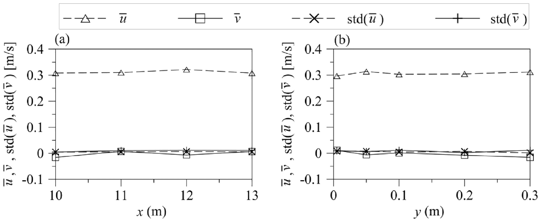
Current alone flow in preliminary experiment at z/h = 0.5: (a) x-direction (y = 0.3 m) and (b) y-direction (x = 12 m).
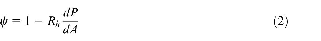
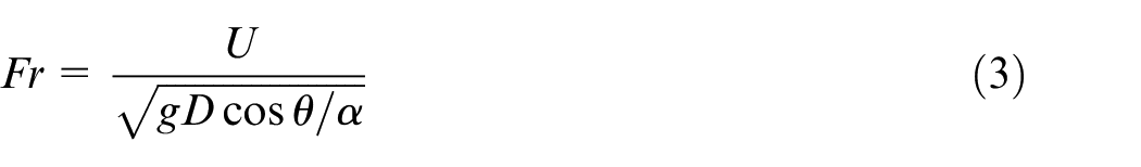
Also, the stability of the incoming uniform flow in the channel was verified by the equation (1),38,39 derived by Vedernikov 40 using an approximation of the Saint-Venant equation.

Where
Where
The wave generation by the installed plunger type wavemaker was validated with the second order Stokes wave theory for pure wave case without current. Therefore, an experiment was performed in the flume for wave alone (WA) case using the experiment methodology as reported in Sarkar et al.
41
using the same experimental set-up. The water depth was kept at 20 cm and the oscillation time period of plunger of the wavemaker was set as T = 1.23 s (
The velocity potential (
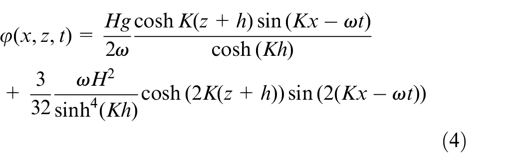
Here H is the wave height and
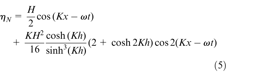
The second order Stokes wave theory is applicable at intermediate depths (
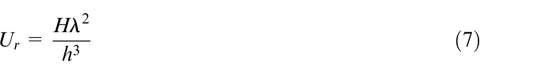
Here in the present experiment for wave alone case, the Ursell number is approximately equal to 2.85 and follows the Ursell number criteria to apply second order Stokes wave theory.
Using the equation (5), for the experimental wave characteristics,
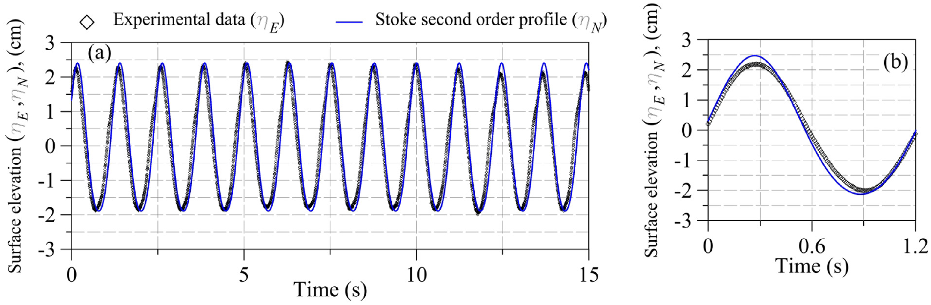
(a) Comparison of surface elevation between experimental and analytical (Stoke second order equation) at wave steepness, H/λ = 0.061, (b) comparison of ensemble average wave cycles of surface elevation profile between experimental and analytical.
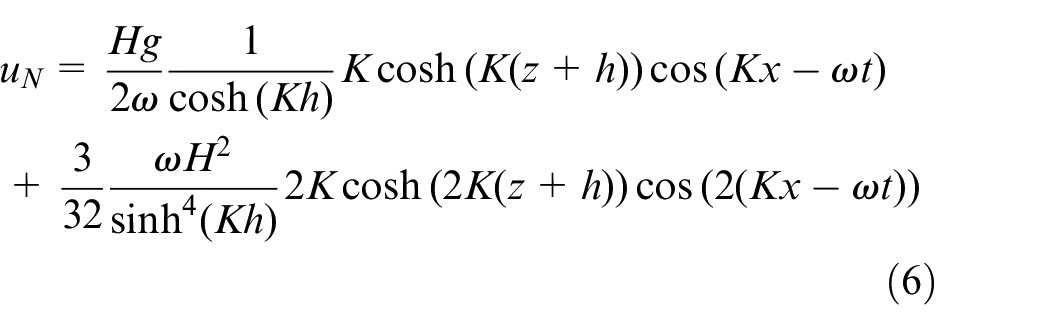
Using the equation (6), the longitudinal direction velocity (
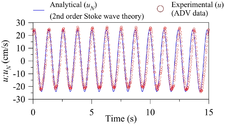
Comparison of longitudinal velocity between analytical and experimental results for wave steepness, H/λ = 0.061 at z = −10 cm.
For the detailed experimental study on the turbulence structure on the side wall boundary layer due to the effect of d-type rib roughness for the wave-current combined flow two types of wave-current combined flow situations were considered and were designated as as WCC0.4 and WCC0.8. The WCC0.4 and WCC0.8 cases correspond to surface wave frequency f = 0.4 and 0.8 Hz superimposed respectively into the current alone flow. The wave characteristics for each type of wave-current combined flows are given in Table 1.
Wave characteristics at test section.
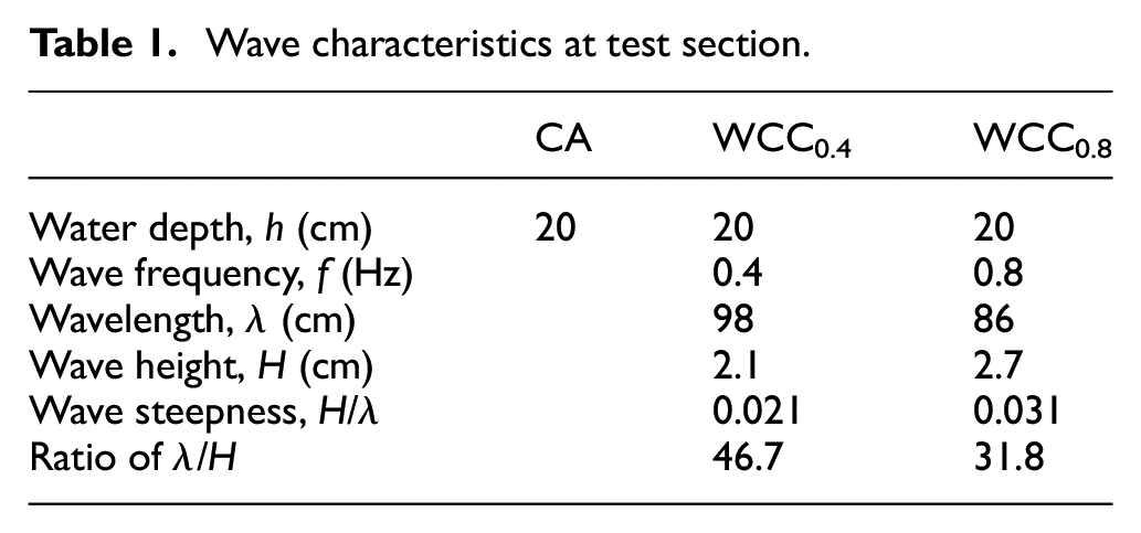
The wavelength (λ) and wave height (H) of the wave-current combined flow are estimated from the captured images of progressive waves. To record the photographs of the progressive waves, a digital camera was focused perpendicular to the flume’s Perspex side wall. The photos had a resolution of 1280 × 720 DPI. The average wavelength and waveheight are calculated by first converting each image’s pixel unit to the metric unit (1 pixel = 0.026458 cm) and then averaging the results. The uncertainty of the computed averaged wavelength and wave height for both wave frequency cases are within 2%. The calculated wave steepness for WCC0.4 and WCC0.8 cases are 0.021 and 0.031, respectively (Table 1), and these values are much less than the limiting criteria (0.14) of wave breaking.50,51 The ratios, λ/H = 46.7 and 31.8, obtained for WCC0.4 and WCC0.8 respectively, are well within the range of 4–56 proposed by Goda
52
for waves in natural settings. It is worthwhile to distinguish the wave regions based on the ratio of water depth and wavelength (h/λ) as shallow water, intermediate depth and deep-water wave regions.
42
The present wave cases represented intermediate (
Measurements and methodology
The three components of velocity u, v and w corresponds to x, y and z direction were measured by the side looking 16 MHz micro-acoustic Doppler velocimeter (ADV). The three receivers of ADV system records simultaneously velocity component, signal strength, signal-to-noise ratio (SNR) and correlation value. The SNR and correlation values are used primarily to determine the quality and accuracy of the velocity data. 53 The minimum values of SNR and correlation are usually 15 dB and 70% that is required to record signals for turbulence characterization purposes. 54 Hence, the values of SNR and correlation lower than 15 dB and 70% are considered as poor-quality data which may lead to wrong interpretation in results. Also, in the ADV recorded velocity signals, there may be spikes caused by aliasing the Doppler signal and these spikes create ambiguity in the record.55,56 Thus, the removable of poor-quality data and spikes from the record data is required to show the reliability of the quantitative results. The phase space threshold despiking developed by Goring and Nikora 56 is used to remove spikes from the 3-min recorded data. Also, to remove the plausible noise, the raw ADV data are processed by high pass filter with low cutoff signal-to-noise ratio (<15 dB) and correlation samples (<70%) and this is implemented by Win-ADV software. To visualize the consequence of filter process, an example of a record data of ADV for current alone flow situation shown in Figure 5.
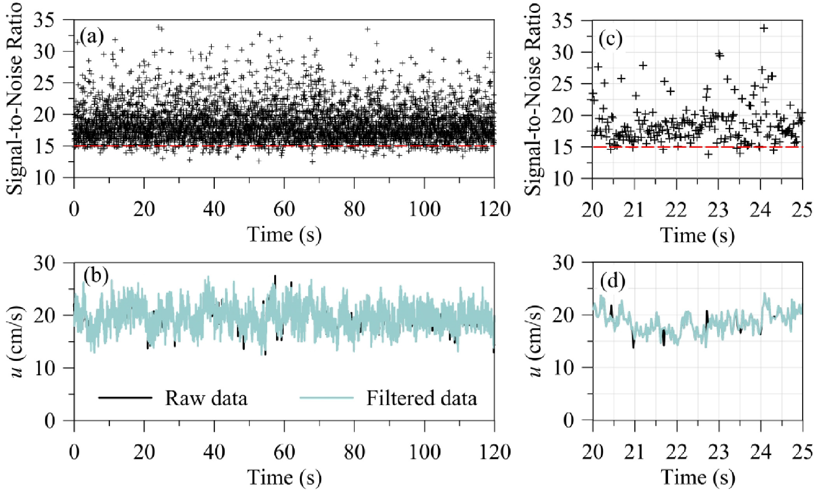
Sample record dataset of ADV used for filter test (a) signal-to-noise ratio data (b) overlapped plot of raw (unfiltered) data and filtered data of u velocity, (c) signal-to-noise ratio for small length of time 5 s and (d) overlapped plot of raw and filtered data for small length of time 5 s.
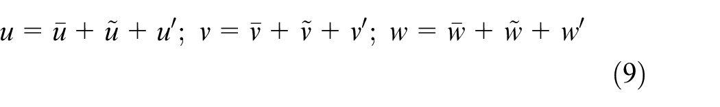
Figure 5(b) shows the comparison plot between raw ADV data and filtered data of u and Figure 5(a) shows their corresponding SNR value for length of 120 s. In the Figure 5(a) symbols (+) represents the SNR values and the dash-line (red color) is the low cut-off (15 dB) line. It means below the dash-line the SNR values and corresponding velocity (u) data are poor quality data, hence this data must be filtered from the record. To compare the filtered and raw data, the filtered timeseries data is overlapped with the raw data as shown in Figure 5(b). It is observed from the Figure 5(b) that the black spots in the overlapped timeseries data are actually eliminated data those have low SNR value (<15 dB) in raw timeseries data. For clarity of visualization a small length 5 s timeseries data are plotted in Figure 5(c) for SNR value and Figure 5(d) for velocity for comparison between raw and filtered data. In the present study to characterize the turbulence structure, the analysis was performed on the filtered data set. The velocity components u, v and w are decomposed into its mean and fluctuation parts as

Here
Here tilde (∼) sign denotes wave-induced velocity. Since the wave-induced velocity is periodic in nature, it can be calculated from the phase averaged velocities 19 as
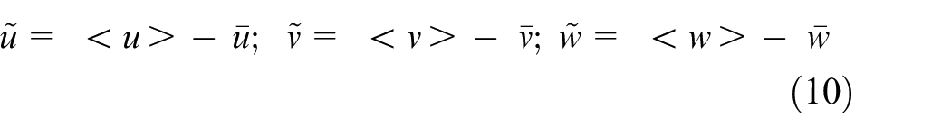
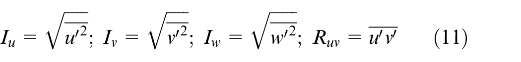
where the angle bracket (< >) represents phase averaged velocities. Turbulence intensities and Reynolds shear stresses are estimated from the turbulent velocity fluctuations. Accordingly, the streamwise (Iu), transverse (Iv) and vertical (Iw) turbulent intensities and the Reynolds shear stress (Ruv) in the x-y plane are expressed as
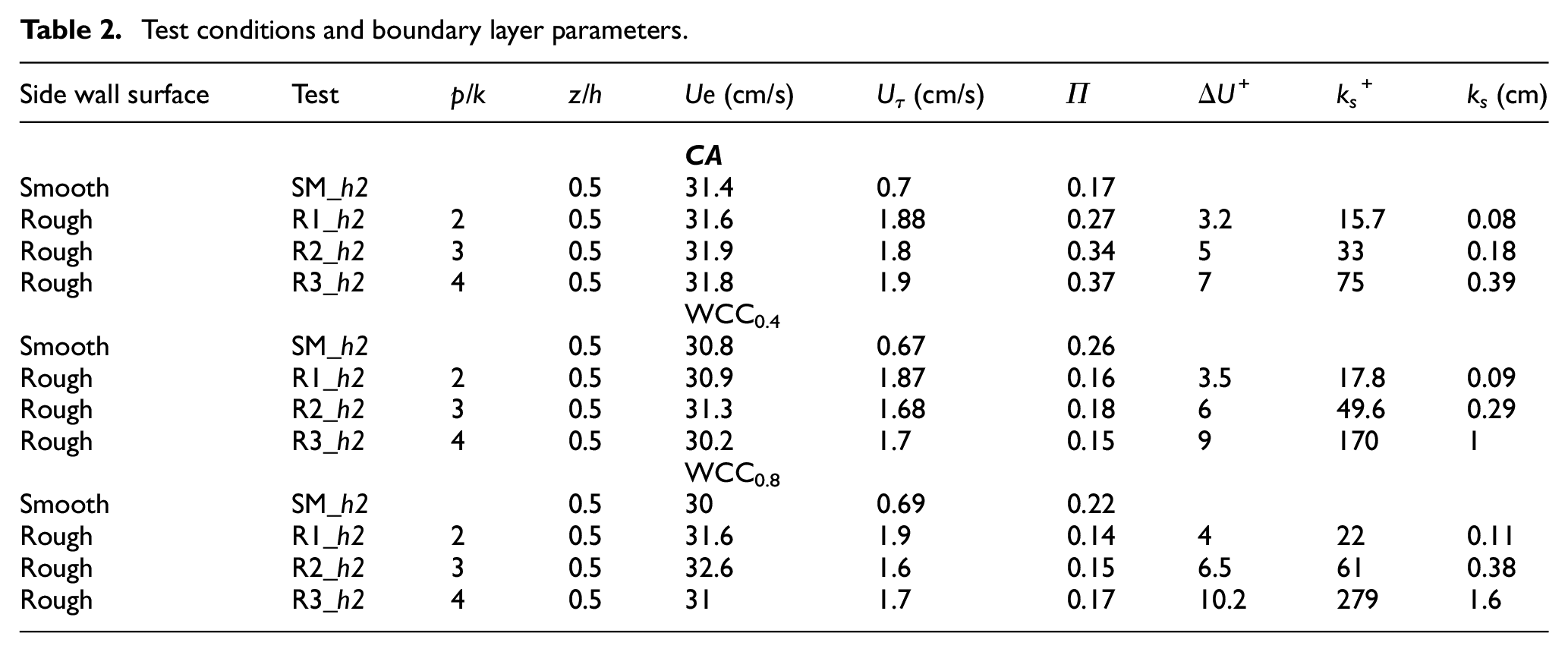
The details of all experimental test conditions and boundary layer parameters are summarized in Table 2. In the forthcoming discussion as well as in Table 2, SM, R1, R2, and R3 refer to the test case with smooth side wall, the cases of rough side walls with p/k = 2, p/k = 3, and p/k = 4, respectively. The mean velocity and the turbulent quantities were measured carefully over smooth side wall (SM) and rough/ribbed side walls (R1, R2, and R3) for current alone flow (CA) and wave-current combined flows (WCC0.4 and WCC0.8). All measurements were carried out along the transverse direction (perpendicular to the side wall) midway (xc) between two successive ribs for p/k = 2, 3, and 4 (see Figure 1(c)). The measurement position (xc) was located beyond the distance x = 9.5 m from flume inlet, where the flow was verified to be fully developed. The mean velocity profiles were measured along the transverse direction from the closest possible position (y/B = 0.015, where y = normal distance from the wall and B = half of channel width) of side wall to center line of channel at three different heights (h1, h2, and h3) of water for p/k = 2, 3, and 4. The three different heights h1, h2, and h3 are defined as z/h = 0.25, z/h = 0.5 and z/h = 0.75 respectively, where z = height from bottom bed and h = water depth. In this paper, the analysis is performed considering measured data at height h2 (z/h = 0.5) which we defined as mid-depth data.
Test conditions and boundary layer parameters.
The shear velocity, Uτ for smooth wall surface is determined using the Clauser chart method 57 assuming the velocity profile follows the logarithmic form (equation (12)) in the overlap region of the boundary layer. 58
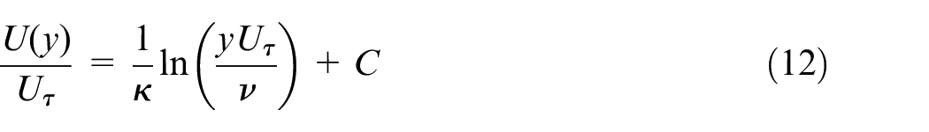
Here,
where
The mean velocity profile in inner coordinates (Y+ vs U+) for smooth and rough boundary wall surfaces at h2 (SM_h2, R1_h2, R2_h2, and R3_h2) for CA, WCC0.4 and WCC0.8 flow cases are shown in Figure 6. In this figure (Figure 6),
Here
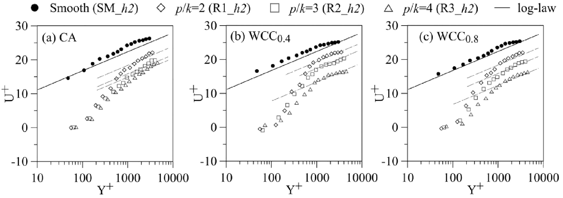
Mean velocity profiles in inner coordinates. Solid lines are log-law (U+ = 2.44lnY++ 5) for smooth wall surface: (a) CA, (b) WCC0.4, and (c) WCC0.8.
Results and discussions
Mean velocity distribution
The streamwise mean velocity profiles in outer coordinates for all the test conditions are shown in Figure 7. The measured freestream velocity (
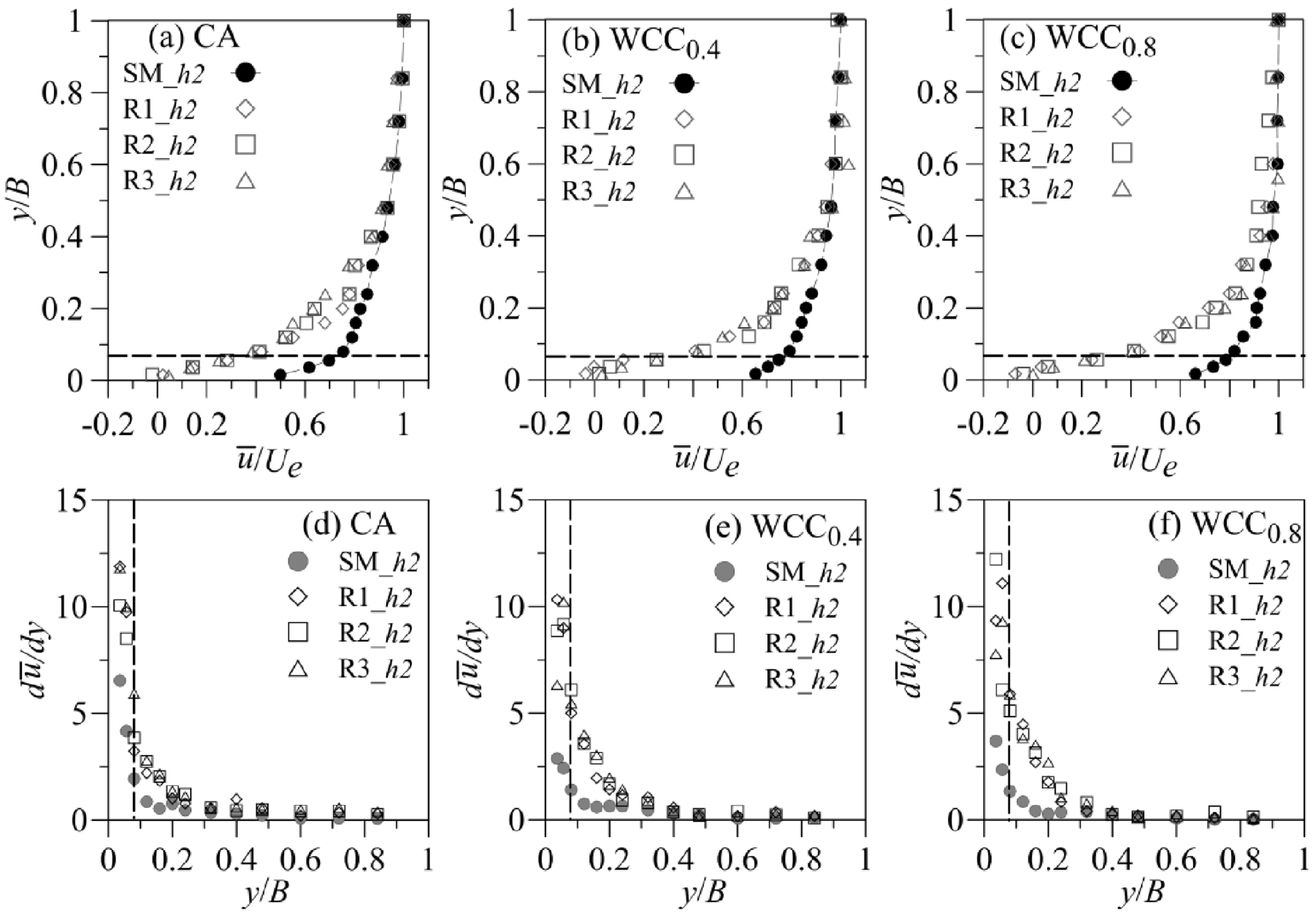
Normalized mean velocity profiles over smooth and rough surfaces for (a) CA, (b) WCC0.4 and (c) WCC0.8 flow cases in outer coordinates and velocity gradient profiles for (d) CA, (e) WCC0.4, and (f) WCC0.8.
Figure 7(a) shows that mean velocity profiles over rough walls have smaller magnitudes than smooth wall profiles toward the wall boundary, indicating that roughness has a significant impact on the shape of velocity profiles near the wall boundary. The velocity decreases due to momentum deficit caused by the roughness. 61 Similar results are found for wave-current combined flow (Figure 7(b) and (c)). Figure 7(a) to (c) reveals that the major deviation of mean velocity profiles for rough walls compared to that for smooth wall profiles are nearly upto y/B = 0.3 and beyond y/B>0.3 the same deviation is almost negligible. As a result, the velocity profile for smooth wall and rough walls are almost same in the outer region of the boundary layer. These observations imply that the impact of p/k = 2, 3, and 4 roughness is limited to the region of y/B<0.3 for the presented current alone and wave-current combined flow. The roughness sublayer is defined as the region typically 5 times of roughness height from the wall in the rough-wall turbulent boundary layer 11 and in the present experiment this roughness sublayer is found based on above as y/B<0.25 region of the boundary layer. Thus it is evident from Figure 7(a) to (c) that the effect of p/k = 2, 3, and 4 (d-type) rib roughness on the mean velocity profiles are majorly confined to the roughness sublayer and beyond this sublayer the profiles are almost collapsed. Li and Li 65 reported in their study that within the roughness sublayer of d-type roughness, the velocity profile follows a quasi-linear distribution and beyond the roughness sublayer multiple profiles collapse into one. It is clear from Figure 7(a) to (c) that the negative velocities occur inside the ribs’ cavity region representing the flow reversal. 66 The magnitude of maximum negative velocity for current alone flow is about 3% of the free stream velocity whereas for wave-current combined flow it is about 7% of free stream velocity. The magnitude of negative velocity is relatively high for wave-current combined flow compared to current alone flow and may be due to the presence of orbital velocity in the wave-current combined flow condition.3,24
The mean velocity gradient,
Turbulence intensities
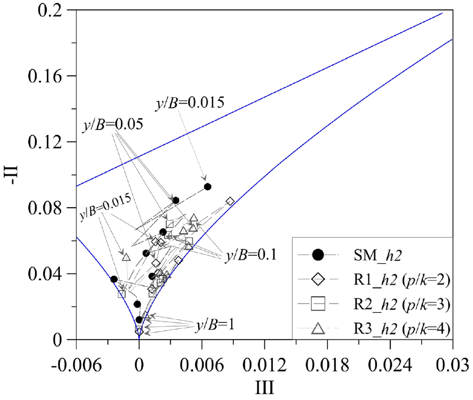
Figure 8 shows the profiles of normalized turbulence intensity in the streamwise direction,
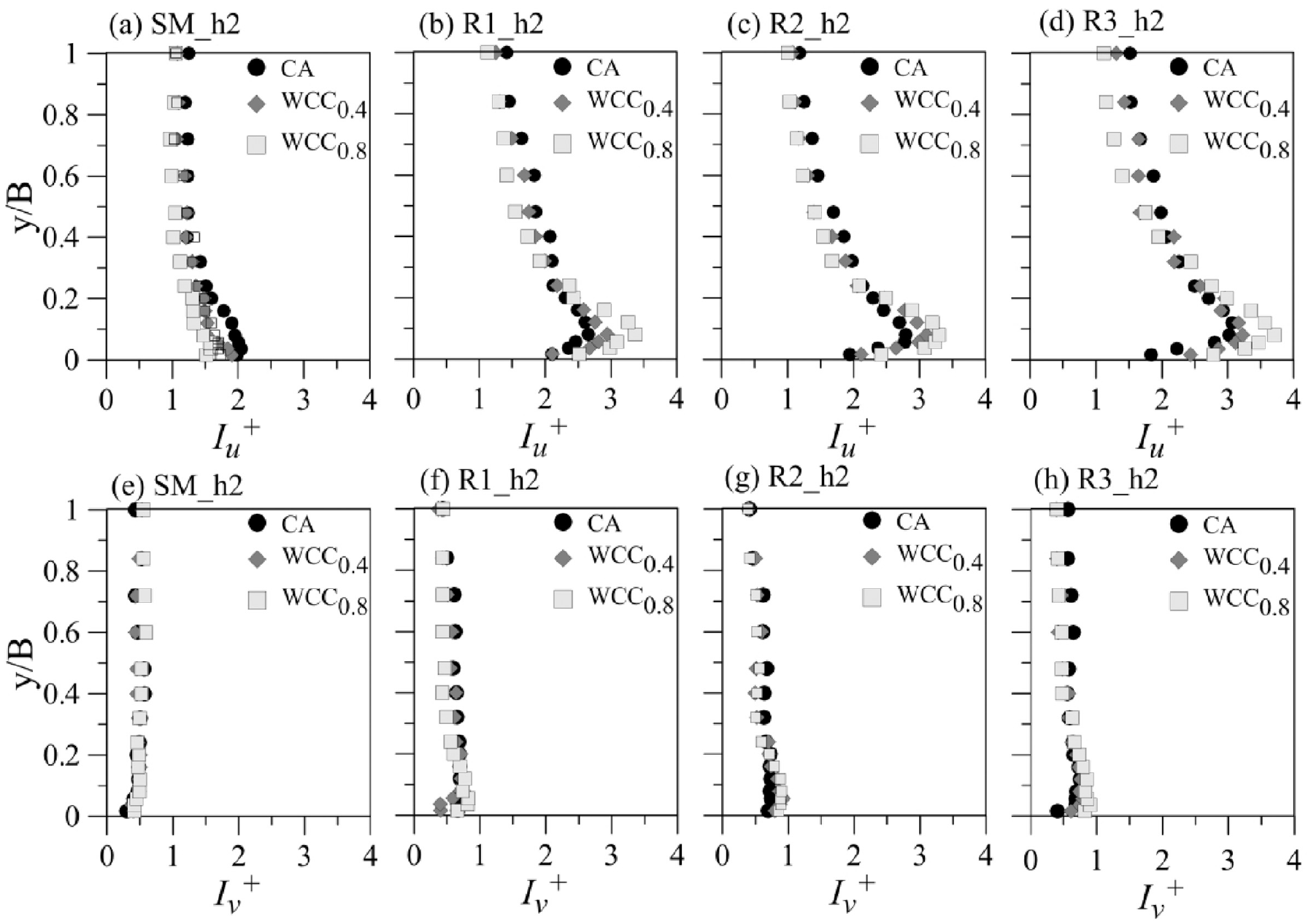
Normalized streamwise turbulence intensity profiles over (a) smooth and (b-d) rough surfaces for CA, WCC0.4 and WCC0.8 flow cases. And normalized wall normal turbulence intensity profiles over (e) smooth and (f-h) rough surfaces for CA, WCC0.4 and WCC0.8 flow cases.
For wave-current combined flow (both WCC0.4 and WCC0.8) over the d-type rough side wall (Figure 8(b)–(d)) the streamwise turbulence intensity
In the rough boundary wall, the addition of even smallest wave height with the current alone flow caused a spectacular increase in turbulence intensity compared to that of current alone flow.
3
The addition of waves to the current probably imposes additional turbulence scales through nonlinear interaction with the turbulence field of the current alone flow under roughness influence resulting in enhanced turbulence intensity at the near side wall region. Pertinent to these Figure 8(b) to (d) shows that large
The wall normal turbulence intensity (
Reynolds shear stress
In Figure 9 the profiles of normalized Reynolds stress (
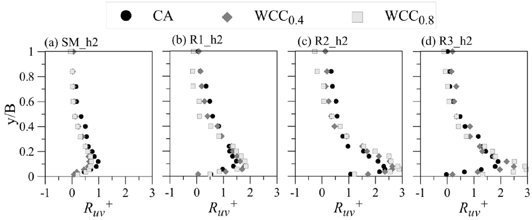
Normalized Reynolds shear stress profiles over smooth and rough surfaces for CA, WCC0.4 and WCC0.8 flow cases: (a) SM_h2, (b) R1_h2, (c) R2_h2 and (d) R3_h2.
TKE dissipation rate (ε) estimation
In order to understand the effect of d-type rib roughness under the wave-current combined flow on TKE (turbulent kinetic energy) dissipation rate (ε), equation (15) is used to estimate the TKE dissipation rate assuming the local isotropy. 73
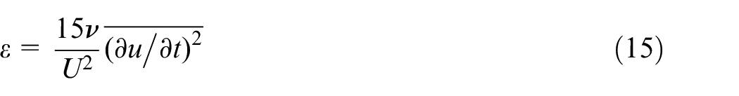
Thereafter, the obtained TKE dissipation rate, ε, is made dimensionless by B and Uτ,
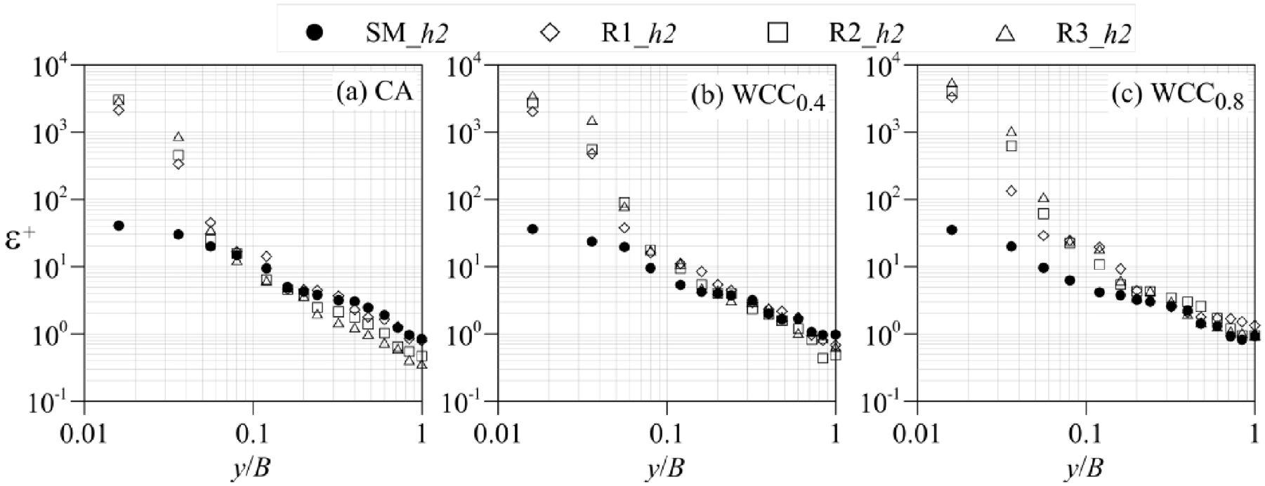
Profiles of normalized TKE dissipation rate, ε+ = εB/U3 τ over smooth and rough surfaces for (a) CA, (b) WCC0.4, and (c) WCC0.8 flow cases.
Figure 10 reveals that for rough surfaces R1, R2, and R3, the magnitudes of
Turbulent length scales
In view of the energy cascade introduced by Richardson, 74 the turbulence can be considered to be composed of eddies of different sizes. The various sizes of eddies are characterized by the different scales of motion. The largest size of eddies are defined by the integral length scale at which the kinetic energy is produced. According to Richardson, 74 the large eddies are unstable and break up into smaller eddies by transferring their energy. The smallest size of eddies are defined by the Kolmogorov length scale and at this length scale the energy is dissipated. The intermediate size between largest and smallest size eddies are known as Taylor scale. 75 The physical interpretation of Taylor scales is not so clear. Mainly it is used to define the Taylor scale-Reynolds number which is used in grid generated turbulence. 75 Kolmogorov, Taylor and integral length scales play an important role to characterize the structure of turbulence. The present study focuses on the distribution of typical turbulent scales across the side wall boundary layer under both current alone flow and wave-current combined flow over smooth and d-type rough boundary. The present study also emphasizes on the effect of increasing spacing between two ribs in the side wall rib roughness and a comparison is made with the without rib-roughness side wall in the context of changes observed in the turbulence length scales.
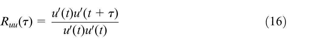
The streamwise integral length scale (Lu) is determined following the estimation of the integral time scale. The integral time scale is calculated by integrating the data
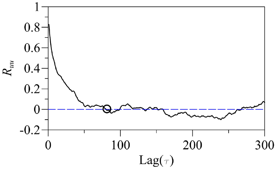
Streamwise autocorrelation function for test run SM_h2 at y/B = 0.03 for CA flow case. Dashed line represents the zero-line. Circle denote the first zero-crossing point of Ruu.
The streamwise velocity component
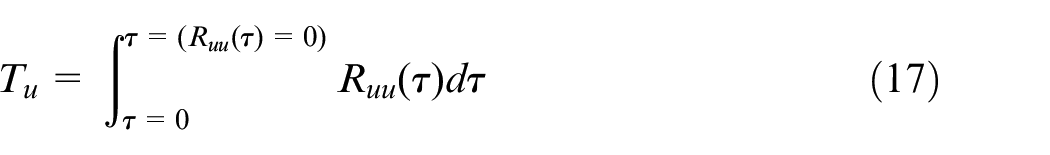
where
Figure 12 shows the distribution of
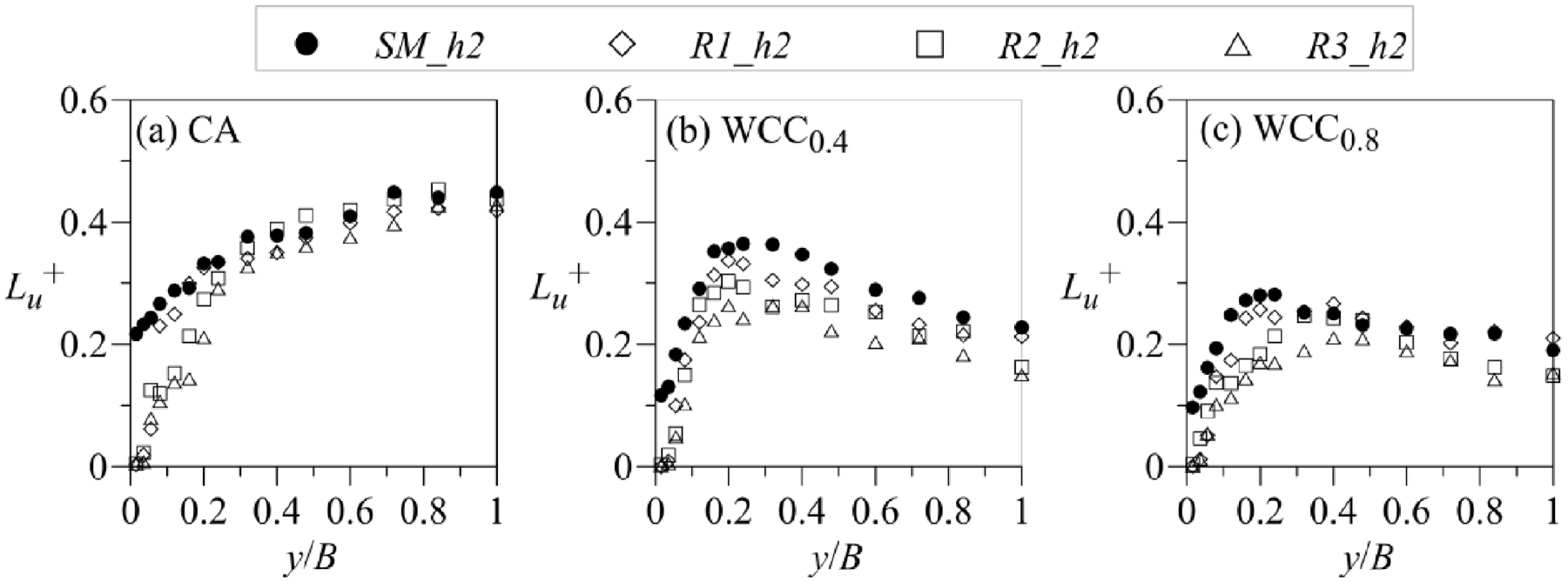
Normalized streamwise integral length scale profiles over smooth and rough surfaces for (a) CA, (b) WCC0.4 (c) WCC0.8 flow conditions.
The smallest size of eddies known as Kolmogorov length scale (η) is calculated from the estimates of dissipation rate (ε) obtained from equation (15). The Kolmogorov length scale is given by
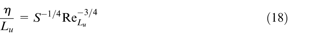
where
Normalized Kolmogorov length scale profiles over smooth and rough surfaces for (a) CA, (b) WCC0.4 (c) WCC0.8 flow conditions.
Figure 14 shows the profiles of normalized Taylor length scale (
Here,
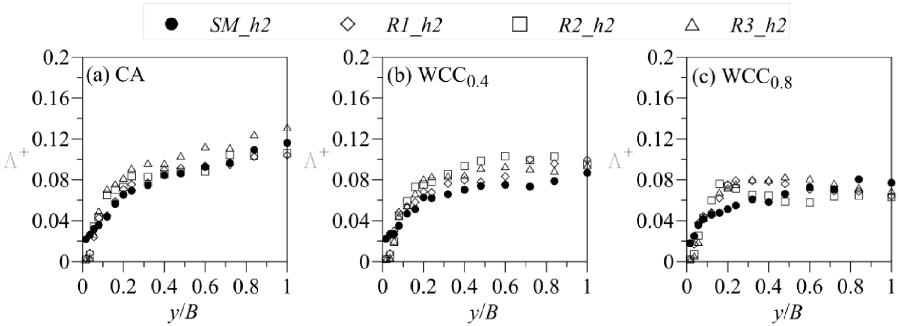
Normalized Taylor length scale profiles over smooth and rough surfaces for (a) CA, (b) WCC0.4 (c) WCC0.8 flow conditions.
Streamwise integral, Kolmogorov and Taylor length scale distribution with respect to the wall normal distances (y/B) from the side wall of the channel are shown in Figures 12 to 14 respectively. The rate of transfer of turbulent kinetic energy and the energy dissipation rate can be related to the characteristic length scale for turbulent motion. It is observed that length scales in the proximity of side wall region for all roughness cases (p/k = 2, 3, and 4) are smaller than smooth surface that is, surface without rib roughness, which implies that rib roughness enhances the energy dissipation rate. Furthermore, with the increase of spacing between two ribs a decrease in the length scales is observed. This corresponds to the lower momentum transfer with the increase of energy dissipation rate, for the range of spacing considered in the present study.
Anisotropy of Reynolds stresses
It is of substantial interest to have some prior knowledge on the anisotropy of the flow field for the simulation of turbulent flow over rough surfaces computationally. 7 This knowledge of anisotropy should be useful in identifying the sensitivity of turbulence structure for various boundary conditions, in addition to being relevant in the context of developing turbulence models. 8 Also, the invariant analysis primarily provides information on the anisotropy of the large-scale motion7,8 showed that the turbulence in a rough wall boundary layer is more isotropic than that in a smooth wall boundary layer.
To quantify the level of anisotropy of the turbulence field, Lumley
78
introduced the Reynolds stress anisotropy tensor (
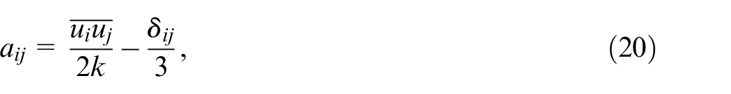
and invariants

Here
Anisotropy invariant map (AIM).
In the present study, the AIM is presented to characterize the state of turbulence for smooth wall boundary and rough wall boundary (p/k = 2, 3, and 4) for both current alone (CA) flow and wave current combined (WCC0.4 and WCC0.8) flow. Figure 16 shows the data for CA flow case and Figure 17 shows the data for wave current combined (WCC0.4 and WCC0.8) flow cases. Data in Figures 16 and 17 represent different y/B locations considering transverse direction outward from the side wall to center line of channel for both smooth wall and rough wall boundary cases. Pertaining to the data points in Figures 16 and 17, location y/B = 0.015 represents the near wall data for smooth wall boundary and for rough wall cases it represents the data point that lies in the cavity region for p/k roughness within the roughness elements. Similarly the location y/B = 0.05 and y/B = 1 indicate the data point of rib-crest line and center-line of channel width respectively. Further y/B = 0.1 indicates the 1k (one times of rib height) distance from the rib-crest line which is within roughness sublayer. In the Figure 16, the magnitudes of –II and III differ considerably between smooth and rough surfaces for CA flow case. For the smooth surface, the tendency of data of AIM (–II and III) is to decrease with the increase in y/B moving outward from the wall. For the rough surfaces (R1, R2, and R3), the pattern of data of AIM is quite similar to that of smooth surface. Figure 16 shows smaller magnitudes of –II and III in the far wall region, which results in data concentration at the bottom cusp region of AIM. The data for location y/B = 1 is close to the axisymmetric line. This result agreed with study of Krogstad and Torbergsen 7 invariant analysis of wall bounded turbulent flow by Krogstad and Torbergsen. 7 They documented that the central region of a fully developed pipe flow follows the axisymmetric line and anisotropy increases toward the wall. Figure 16 reveals that close to the side wall, the data shift away from the axisymmetric line and approach two component turbulence showing increased magnitudes of –II and III. In this regard, the smooth wall has maximum magnitudes of –II and III at near wall region (y/B = 0.015) which corresponds to higher anisotropy compared to rough wall cases (R1, R2, and R3) as these rough walls experiences low magnitudes of –II and III. At y/B = 0.015, the state of turbulence largely vary for smooth surface and rib roughness because for rough surface this position corresponds to the region within cavity formed by rib roughness elements. Thus, it is evident from Figure 16 that the data within the cavity region follows the left axisymmetric turbulence line of the AIM closely and move toward the bottom cusp with the increase of y/B from 0.015 to 1. From Figure 16 it reveals that the shape of Reynolds stress changes to “sphere like” from “ellipse like” for smooth wall and from “disk like” for rough wall with the increase of distance from the side wall. 75 From Figure 16 it is further reveal that change in rib spacing shows low sensitivity to the change of anisotropic structure of turbulence. Further work probably is required with a greater number of variations of p/k ratio to understand the effect of rib roughness in modulation of the anisotropic structure of turbulence.
Anisotropy invariant map (AIM) of Reynolds stress tensor for smooth and rough surfaces boundary wall for current alone (CA) flow.
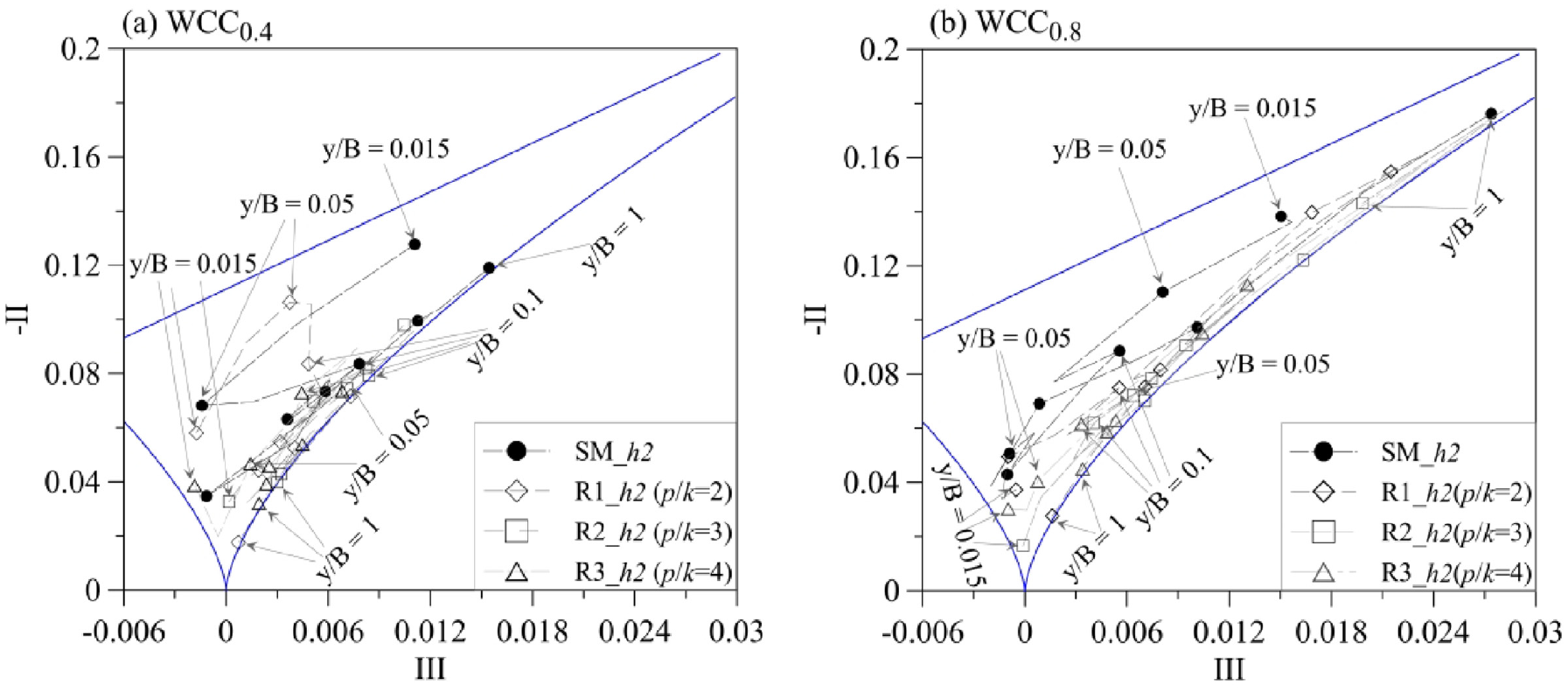
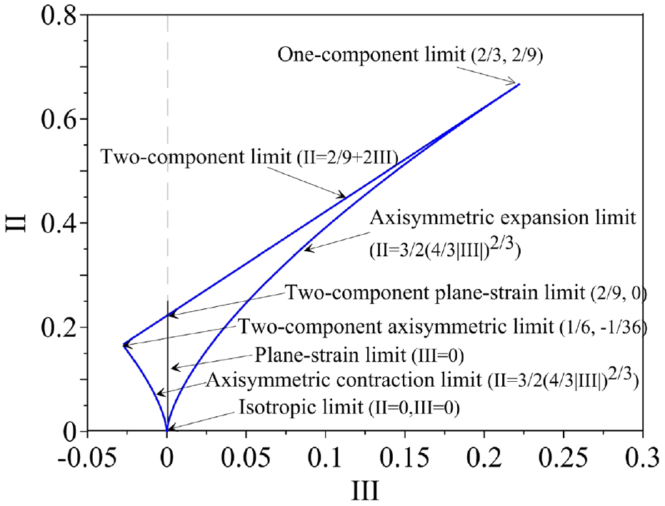
Anisotropy invariant map (AIM) of Reynolds stress tensor for smooth and rough surfaces boundary wall for wave current combined flow (a) WCC0.4 and (b) WCC0.8.
Figure 17(a) and (b) show the AIM for wave-current combined flow cases WCC0.4 and WCC0.8 respectively. For wave current combined flow cases, comparable features are observed as that for current alone flow case. Figure 17(a) and (b) show that majorly the data points are distributed in a wider range along the right axisymmetric line of the AIM compared to CA flow case (Figure 16) where mostly the data points are confined in a small region of AIM. This result (Figure 17) implies that when the wave frequency 0.4 Hz (WCC0.4) and 0.8 Hz (WCC0.8) are added individually to the current alone flow, the state of turbulence is modulated for each case showing larger magnitude of –II and III in AIM for wave current combined flow cases compared to that for CA flow case. Furthermore, the WCC0.8 shows the higher magnitudes of –II and III compared to WCC0.4 which implies that increased level of anisotropy dominates when higher wave frequency 0.8 Hz is superimposed to the current alone flow. Similar to CA flow case, for the wave current combined flow cases (WCC0.4 and WCC0.8) also in general, the magnitudes of –II and III data for smooth wall surface are significantly larger than that over rough wall surfaces. The data adjacent to the side wall (i.e. y/B = 0.015) starts from the threshold region of two component turbulence and move toward the right axisymmetric limit line following a certain trajectory with increasing distance from the side wall. It is evident from Figure 17(a) that at y/B = 1, the data follow the right axisymmetric line indicating the one component turbulence with “cigar-shaped” turbulence. In contrast with the smooth wall surface, the data adjacent to the side wall starts from the region close to the left axisymmetric limit line for ribbed wall cases. In the cavity region (y/B = 0.015 for ribbed rough surfaces) often the streamwise component of fluctuating velocity is smaller than the other two lateral components 7 and this possibly leads to the data for this location to align with the left axisymmetric turbulence line of AIM. Moreover Smalley et al. 83 reported that the state of turbulence below the crest plane that is, cavity of d-type roughness approach axisymmetric turbulence. Further they also reported that at the near wall recirculation region, two components axisymmetric turbulence is approached. Apparently for WCC0.8 flow cases (Figure 17(b)) the data follows similar trend as that for WCC0.4 (Figure 17(a)) with the little modulation of the magnitudes of –II and III indicating increased anisotropy with the increase of wave frequency. Close inspection of Figures 16 and 17 reveal that the level of anisotropy of turbulence in streamwise direction over both the smooth wall surface and rough surfaces for wave current combined flow is more compared to current alone flow. This result agreed well with study of Paul et al. 84 The state of turbulence adjacent to the rib crest line (y/B = 0.05) for both the current alone and wave-current combined flow cases demonstrate a remarkable shift from left axisymmetric turbulence to right axisymmetric turbulence. This change of state of turbulence can be characterized as transformation from “pancake-shaped” turbulence to “cigar-shaped” turbulence according to Choi and Lumley’s 85 description of turbulence. The reason behind this transformation may be attributed to the flow separation from just above the roughness elements of d-type rib roughness in streamwise direction. 66
Conclusions
In this study, a background experiment for wave alone case is performed to compare the second-order Stoke wave theory apart from the actual experiment objective, that is, to understand the effect of d-type rib roughness side wall on the turbulence structure for wave current combined flow. The transverse profiles (i.e. proximity of side wall to half of channel width) of mean velocity, turbulence intensity and Reynolds shear stress have been presented for the wave-current combined flow over the side wall rib rough boundary in order to examine the turbulence characteristics due to combine effect of wave-current flow and rib spacing at near wall boundary. The rib spacing was varied such that pitch-to-roughness height (p/k) ratios were 2, 3, and 4 representing d-type roughness. Two different wave-current combined flow cases wave frequency 0.4 and 0.8 Hz were explored. The transverse profiles were explored for mid water depth over both smooth and rough (p/k = 2, 3, and 4) side wall surfaces and for both current alone flow and wave-current combined flows. The results for rough boundary wall and wave-current combined flow have been compared with the smooth boundary wall and current alone flow cases to illustrate the effect of rib spacing and wave-current combined flow. The study of Reynolds stress anisotropy and the turbulent length scale distributions over the smooth surface and p/k rib roughness surfaces for wave current combined flow enrich the existing knowledge on turbulence characteristics near side wall ribbed rough surface under wave-current combined flow. The major findings of the study are given below.
In the background experiment for wave alone case, the wave produced by the wavemaker (cylindrical plunger type) is verified with the second-order Stoke’s wave theory. The free surface elevation and longitudinal velocity obtained from experiment agreed well with analytical result of second order Stoke wave equation.
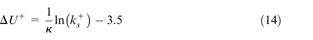
Equivalent sand-grain roughness height (ks) increases with the p/k ratio for both current-only flow and wave-current combined flow. For a given p/k, wave-current combined flow yields higher ks when compared with the current alone flow. Higher wave frequency (f = 0.8 Hz) leads to greater ks (=1.6).
Presence of ribs reduces the streamwise mean velocity near the rough (ribbed) side wall of the channel as compared to a smooth wall case. This mean velocity deviation remains confined within a region (known as roughness sublayer) having approximate thickness 5k (where, k is roughness height). The mean velocity gradient,
For a channel with smooth side wall, the streamwise turbulence intensity near the side wall is relatively lesser for wave current combined flow compared to current alone flow. For ribbed wall, the wave-current interacting flow induces higher turbulence intensities compared to that induced by current alone flow. Further pitch to roughness height ratio influences the streamwise turbulence intensity for both current alone flow and wave-current combined flow. Present experimental results reveal that the near wall turbulence intensity increases with the superposition of wave on current compared to current alone flow due to the mutual interaction between rib roughness and wave current combined turbulence field. This probably occurs due to the addition of turbulence scales due to the interaction of wave with the roughness elements on the background turbulence. Moreover, turbulence intensity increases sharply near the wall as p/k ratio increases, which are true for both current-only flow and wave-current combined flow. Variation of Rreynolds shear stress with p/k ratio and different wave-current combinations are similar to that of streamwise turbulence intensity. For rib roughness, the peak value of shear stress profile lies nearly along the rib crest line and on both side of the crest line the shear stress value decreases asymptotically.
Wall roughness leads to substantially high TKE dissipation rate in the near wall region, as shown in Figure 10. Since wave-current combination enhances the equivalent sand-grain roughness height (ks), the dissipation rate also increases in both near wall (boundary layer) region as well as core region of the channel for wave-current interacting flows, particularly for rough side-wall cases.
The effects of side wall roughness and wave interaction on the streamwise integral length scale or the largest eddy size are demonstrated through Figure 12. It is evident that the smooth side wall results in highest integral length scale. As the roughness (p/k ratio) increases, integral length scale decreases for both current alone flow and wave current combined flow. One of the most interesting findings of the present study is that the addition of wave reduces the integral length scale for both smooth and rough wall cases. With an increased wave frequency (WCC0.8 case) the largest eddy size is reduced even further. The estimates of smallest or Kolmogorov length scale demonstrate similar effects of wall roughness and wave.
The results of anisotropy invariant map (AIM) of Reynolds stress tensor shows that near wall anisotropy reduced when p/k roughness introduced to the smooth side wall. The data adjacent to the side wall is two component turbulence and moves to axisymmetric turbulence with the increase of distances from the wall which imply the change of state of turbulence.
The wave current combined flow produces more anisotropy which reflects in the AIM where the data are distributed in a wide range along the right axisymmetric curve of AIM rather confined in a small region near bottom cusp of this map like current alone flow.
Footnotes
Declaration of conflicting interests
The author(s) declared no potential conflicts of interest with respect to the research, authorship, and/or publication of this article.
Funding
The author(s) disclosed receipt of the following financial support for the research, authorship, and/or publication of this article: The authors would like to acknowledge the Science and Engineering Research Board, Department of Science and Technology, Government of India for the financial support for this research (Contract no: EMR/2015/000266).