
Abstract
This article presents a metocean modelling methodology using a Markov-switching autoregressive model to produce stochastic wind speed and wave height time series, for inclusion in marine risk planning software tools. By generating a large number of stochastic weather series that resemble the variability in key metocean parameters, probabilistic outcomes can be obtained to predict the occurrence of weather windows, delays and subsequent operational durations for specific tasks or offshore construction phases. To cope with the variation in the offshore weather conditions at each project, it is vital that a stochastic weather model is adaptable to seasonal and inter-monthly fluctuations at each site, generating realistic time series to support weather risk assessments. A model selection process is presented for both weather parameters across three locations, and a personnel transfer task is used to contextualise a realistic weather window analysis. Summarising plots demonstrate the validity of the presented methodology and that a small extension improves the adaptability of the approach for sites with strong correlations between wind speed and wave height. It is concluded that the overall methodology can produce suitable wind speed and wave time series for the assessment of marine operations, yet it is recommended that the methodology is applied to other sites and operations, to determine the method’s adaptability to a wide range of offshore locations.
Keywords
Introduction
Metocean models are commonly used to produce data sets for planning, modelling and review of marine operations for a variety of offshore industries. These models are often employed when there is insufficient recorded data for a specific offshore location. Increasing efforts have been made in the offshore wind industry to better predict the uncertainties in the progression of weather sensitive operations. To exemplify, offshore wind installation costs can account for up to one-third of the overall project cost and a better understanding of the potential delays during marine operations will support developers to reduce the levelised cost of energy (LCOE). Future projects are planned for increasingly remote locations accompanied with challenging weather conditions such as high winds and wave heights that can cause significant disruption to a planned operational schedule, thus increasing the overall risk profile for installation or operation and maintenance (O&M) campaigns. It is therefore important that marine operations can be scrutinised in advance to ensure the correct planning, resourcing and equipment decisions can be made.1–3
Operating within metocean conditions brings significant challenges in understanding the variability of the weather characteristics with the combined impact on operational downtimes or health and safety risks. As metocean conditions are site specific, this requires a bespoke assessment for each project and therefore adaptable assessment tools are necessary to simulate the characteristics of each site.
The generation of stochastic metocean time series has been widely researched for a variety of offshore applications. By generating a significant number of stochastic weather series that resemble the variability in key metocean parameters, probabilistic outcomes can be obtained to predict the weather windows, delays and subsequent installation durations for specific tasks or multiple marine operations. In recent years, dedicated probabilistic simulation tools have been developed, to predict the progression of marine operations and the suitability of resourcing strategies against synthetically produced metocean data. Embedding a stochastic metocean model within these simulation tools allows the users to first input observed weather data for a finite number of years and generate many synthetic realisations of the weather to assess the progression of marine operations. Using a stochastic weather model is beneficial as it draws more certainty on predicted outcomes, yet still encloses the random variability that exists within the observed weather data.4–6
To cope with the variation in the offshore weather conditions at each project, it is vital that a stochastic weather model is adaptable to account for seasonal or monthly variations to produce realistic weather time series. The Markov-switching autoregressive (MS-AR) model included in the METIS MATLAB toolbox, developed by Monbet and Ailliot, 7 has been investigated in this study and configured to produce monthly realisations of observed time series. More specifically, we investigate the application of an MS-AR model to produce stochastic wind speed and wave height time series, based on observed data sets. The aim of this article is the implementation and assessment of MS-AR techniques for metocean modelling when assessing offshore wind installations. The MS-AR generated time series is cross examined against a typical offshore operation, to validate the adopted methodology and MS-AR model configurations. By demonstrating that the model is capable of producing characteristics such as the average length of operational weather windows and monthly workability, this supports the case to implement MS-AR metocean models in offshore simulation tools.
To contextualise the application of the MS-AR model, we present a case study on a personnel transfer task from a crew transfer vessel (CTV) to a pre-installed wind turbine transition piece, which is constrained by specified working limits. This task has been selected as it has particularly conservative restrictions and is relevant to a wide range of offshore sectors. The outcomes of completing this task across simulations from three separate sites are first contrasted against the corresponding observed data set, and then the results from three sites are compared to discuss the general outcomes and the overall suitability of the presented methodology. A discussion on the impact of the results for metocean applications and offshore wind risk assessments is presented, and we provide recommendations to build on this study.
Literature review
There has been extensive research on the development and application of environmental models to produce offshore weather series. In Monbet et al., 5 Monbet and Ailliot, the authors of the METIS toolbox, present a review of stochastic models to generate wind and sea state characteristics. Their study begins with Gaussian processes such as the ‘Box and Jenkins’ approach and the ‘Translated Gaussian Process’ (TGP). The Box and Jenkins method is widely regarded as the most classical method where the data are first made stationary by blocking it into monthly or seasonal sets and then applying a Box–Cox transformation. 8 This produces a time series with a Gaussian like marginal distribution, and finally an autoregressive integrated moving average (ARIMA) model is fitted to generate the synthetic time series. An ARIMA model uses the process of differencing many times, to reduce the forecast to an autoregressive moving average process (ARMA). An ARMA model relies on a set number of previous values in a given time series and memory function described denoted by the ‘MA’ or moving average, to produce forecasts. TGP can be described in three steps. For a univariate process, it starts by transforming the observed data into a Gaussian variable, then generating a second-order random time series with the same spectral properties. This second-order time series can then be re-transformed back into a full univariate time series, and it is noted that auto and partial correlation functions may reveal significant differences between the original and synthetically produced data.
It is remarked that while these methods are less sensitive to noisy data, they are reliant on large data sets to generate estimates and have difficulty reproducing an accurate distribution of stormy and calm conditions within the generated time series. Non-parametric methods are investigated including block resampling and resampling Markov chains. Block resampling is described as a method to implement bootstrapping techniques, where each ‘block’ is representative of a time step in the observed data set and random sampling of the blocks are used to reconstruct a sequence of values. This process demonstrates sensitivity to the size of block, as short blocks can struggle to replicate the existence of storms and larger blocks commonly reproduce the observed time series, negating any benefit from employing such models.
Resampling Markov chains such as ‘nearest-neighbour’ are also presented, which begin with a few starting values and searches the data for the nearest lying neighbours to particular points. One of these neighbours is then randomly selected and allocated to the given time step in the series. The authors also discuss the inclusion of selection weighting of closer points by introducing higher probabilities to these values and further sophistications such as the Local Grid Bootstrap method have demonstrated good reproduction of the weather characteristics such as the distribution of storm durations and marginal distributions. Parametric approaches such as artificial neural networks (ANN), MS-AR and generalised autoregressive conditional heteroskedasticity (GARCH) models are promoted for their ability in describing particular weather regimes. ANN models are described for application in short-term forecasts and correcting meteorological models but it is stated that these models are inherently difficult to interpret. Alternatively, MS-AR models and GARCH models are identified as easily interpretable and are capable of restoring the weather regimes similar to those in observed data sets. These models can be reviewed and broken down to understand the embedded computations whereas ANN examples are less accessible for interpretation. However, it is remarked that choosing the correct model types can take some time, by applying steps such as maximum likelihood and least squares. Assessments can be made using the statistical properties from each computation by applying Akaike information criterion (AIC) and Bayesian information criterion (BIC), which provide quantifiable values to identify the best model for the meteorological data.
Ailliot and Monbet 9 investigate the specific application of homogeneous and non-homogeneous MS-AR models to produce wind time series. These models are composed of a blend of autoregressive (AR) models to describe the evolution of the wind speeds over different intervals, and the switching between each AR model is handled by a hidden Markov chain. Their experience highlights that MS-AR models with Gaussian innovations are preferable to those with Gamma innovations due to computational benefits and numerical issues associated with the Gamma case. The study demonstrates the operability of a homogeneous MS-AR model, which is expanded to account for diurnal and seasonal fluctuations by applying a non-homogeneous MS-AR model. The impact of inter-annual variations that can be observed in historical data, associated with climate change, are also considered where they advise the potential inclusion of trend models to improve long term predictions.
Taylor and Jeon 10 investigate various probabilistic forecasting methods for wave height estimates, including kernel density estimation, time-varying parameter regression and various ARMA-GARCH model combinations. Their study considers the suitability of these techniques to support service vehicle mobilisation decisions for offshore wind turbine maintenance campaigns. Kernel density estimation is described as a non-parametric approach and uses kernel smoothing on the empirical distribution of historical data, which can be applied across varying window lengths. A Gaussian kernel function with predefined bandwidth is included in the calculation to control the degree of smoothing applied, and the authors use the continuous ranked probability score to optimise the selection of the bandwidth over a 12-month estimation sample. Time-varying parameter regression models applied to independent estimates of wave height, wave period and wind speed are presented and noted for their relative success in previous short-term forecasting studies. The authors propose three separate models to produce wave height, wave period and wind speed forecast. Each model includes a Gaussian white noise error term and estimated parameters using ordinary least squares. Their models are considered for various lags, with a 4-h lag intended for short-term forecasts and 24-h lag for cyclical predictions.
Univariate ARMA-GARCH models are described for their ability in modelling of autoregression in the mean and the variance of a time series. The authors note that such models are capable of capturing diurnal and annual cyclical patterns and introduce trigonometric terms to account for diurnal behaviour. Maximum likelihood estimates are used to estimate the model parameters, and the Schwarz Bayesian information criterion (SBC) is applied to select the order of the four lag polynomials relating to the AR, MA, GARCH and ARCH components of the model. It is identified that the unconditional distribution of the wave heights in the observed data were not Gaussian and therefore a Box–Cox transformation is applied to reduce skewness and suit the Gaussian distribution. Bivariate ARMA-GARCH models are investigated to account for the dependency between wave heights and the strength of the wind. A vector error correction (VEC) bivariate ARMA-GARCH model is used by the authors, which includes a conditional covariance matrix of the error term, which restricts the prediction of the bivariate outcomes based on positivity of the covariance matrix. For both univariate and bivariate models, the Gaussian, student t and skewed t distributions of the error term are investigated. Assessments of the models are completed using continuous ranked probability, maximum absolute error for point forecast accuracy and a brier score to statistically assess the probability of 1.5-m wave height limit being satisfied. Overall, it is concluded that the most accurate method was the bivariate ARMA-GARCH model for combined wave height and wind speed data.
Mao et al. 11 present a new method to find parameters in the Weibull distribution to produce reliable wind speed statistics and evaluate the benefits of new green shipping concepts using auxiliary wind propulsion. A spatio-temporal transformed Gaussian model was fitted to a 10-year reanalysis of wind time series, which can be applied at fixed positions or along vessel transit routes. The method is validated against wind speeds measured directly by vessels operating in the North Atlantic and Mediterranean Sea. It was found that the method performed better for westbound compared to eastbound voyages, where significant difference was observed against the measured distribution from the vessels. It is concluded that the eastbound inaccuracies can be attributed to captain’s actions and that further assessments should consider the impact of transit route strategies.
De Masi et al.
12
investigate the application of a first order multivariate Markov chain model to produce 20 years of synthetic time series for significant wave height (
Hagen et al.
4
present a multivariate Markov chain model to produce time series for wind speed (
Tzortzis et al. 13 explain that the optimisation of a ships energy system is complicated by time dependencies such as weather conditions and time-varying loads. Their study employs differential algebraic equations and three simultaneous optimisation levels to assess the impact of these dynamic conditions by applying an example weather profile. It is stated that propulsion power is a function of vessel speed and weather conditions, which vary spatially as vessels progress along a route and the optimisation of transit speeds at different intervals can be considered to minimise operating costs. It is recognised that the predominant impacts on vessel speed are wind speed and direction and wave height and direction. The method is adaptable to different weather states, while it is acknowledged that the stochastic nature of the weather conditions is not captured by their simplified deterministic approach.
Leontaris et al.
14
indicate that large observed data sets of approximately 20 years are required in order to produce useful meteorological estimates from a copula model. The scarcity of long observed environmental time series is a key driver for their study, where they use copulas to reproduce multiple years of wind speed (
Methodology
This article applies the homogeneous MS-AR model with Gaussian innovations, embedded within the METIS MATLAB tool box, for application in offshore planning and simulation tools. This section describes the observed meteorological data sets, the MS-AR model tested, the model selection process and a summary of the steps to produce the final time series. It is important to note that the theoretical and computer-based MS-AR models have been adopted for this study. In this article, we present a generic methodology that can be used to generate annual time series of
The main steps of the overall method are shown in Figure 1. A brief summary of these steps are as follows. We begin with observed data that are resampled to three hourly intervals and compiled into monthly sets to obtain stationery, non-seasonal collections. The METIS MS-AR model is first used to assess various model type configurations using the expectation maximisation (EM) algorithm, which are individually evaluated using BIC to identify the most suitable model for each month. The simulation produces 1000 years of synthetic time series of
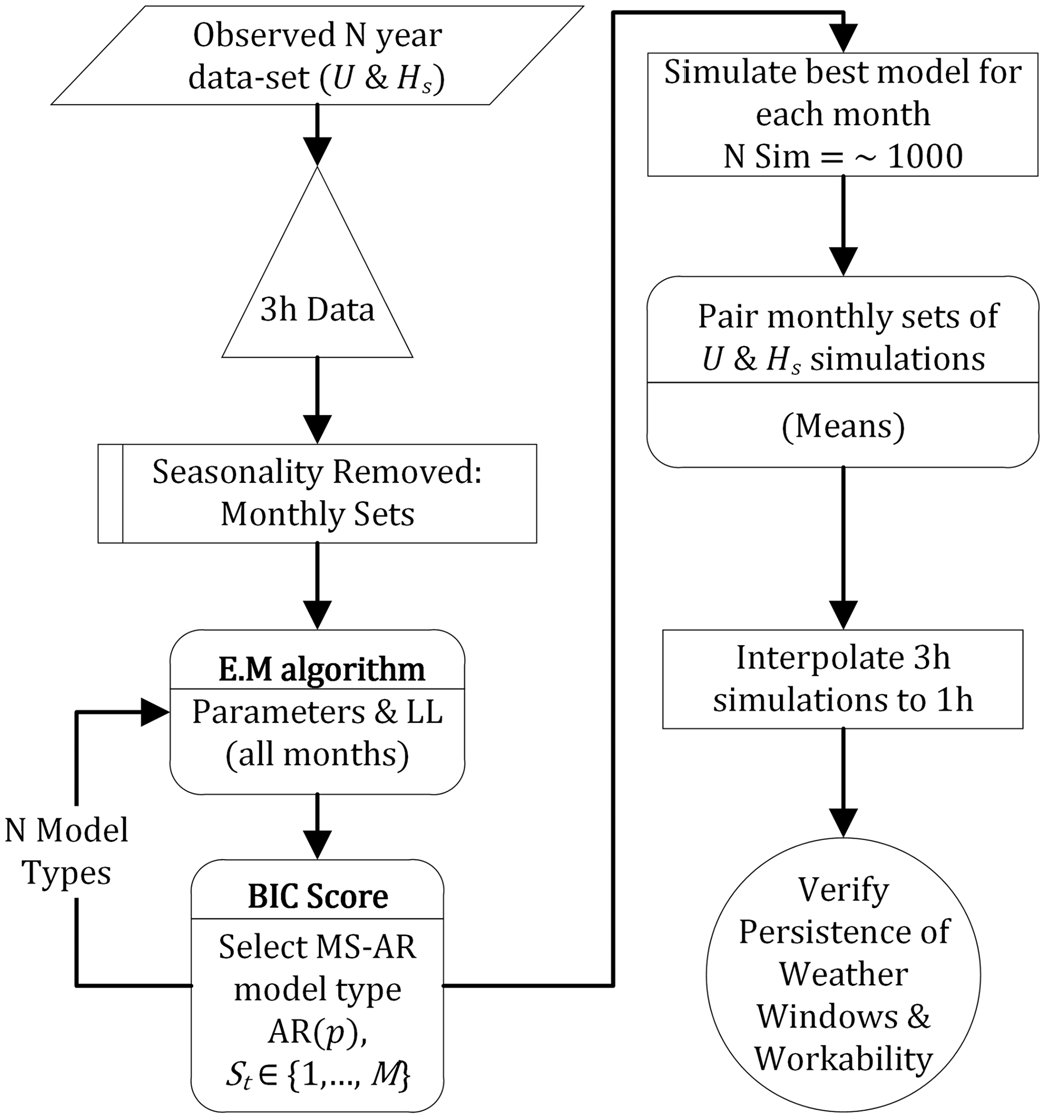
MS-AR modelling and verification methodology.
Data
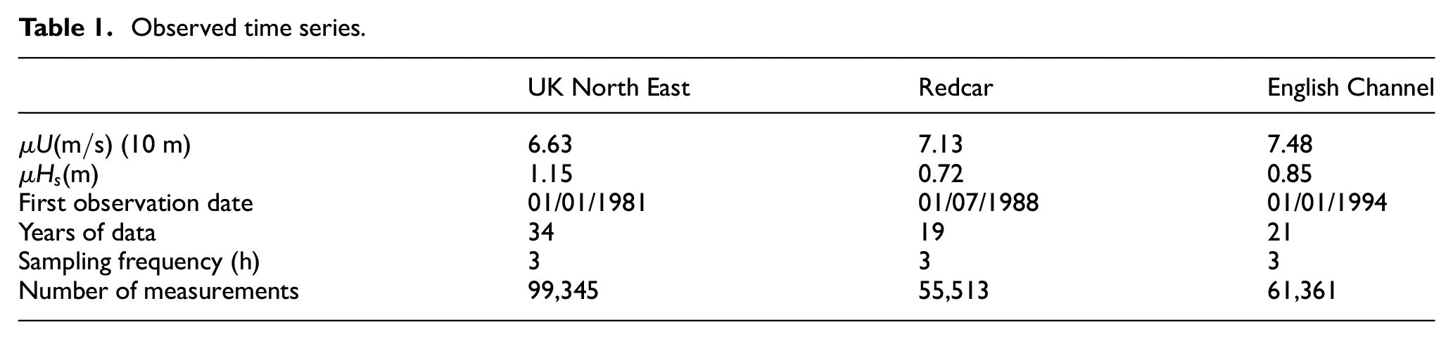
Three different environmental data sets have been sourced to review the consistency of the MS-AR model simulations at various sites with different energies. Wind speed (m/s) and significant wave height (m) are the two meteorological parameters under investigation. The wind speed is taken at a reference height of 10 m, and significant wave height represents the average of the highest third of individual waves over a specified period of time at each site. 15
A summary of each data set is included in Table 1, all of which have a 3-h resolution. These data sets were selected as they are originated from locations close to existing and proposed offshore wind farms. It should be noted that all three data sets were originally recorded at hourly intervals and were subsequently resampled to 3-h observations by extracting the relevant time steps for each day, beginning at 00:00 then every 3 h through to 21:00. Fundamentally, this step reduces the order of the AR model and hence the complexity of the MS-AR model overall. We have chosen the 3-h time step as a compromise between 6- and 1-h intervals. Our experience testing the model has found that the 3-h time step provides a suitable balance between accuracy and simulation time. However, our experience modelling marine operations in various softwares has highlighted that time steps of at least 1 h should be used as an input weather data series, as this provides reasonable resolution for intermediate interpolation, facilitating the simulation of tasks with a time step of less than 1 h. Therefore, it was decided that 3-h results from the MS-AR model would be linearly interpolated to 1-h intervals and compared against the original data sets, originally recorded at an hourly resolution. The validity of this approach is of interest to the authors and follows on from the recommendations of Leontaris et al., 14 who indicate that simulations should be completed at the same scale as the observed data set and then interpolated to the required resolution.
Observed time series.
MS-AR model
This section describes the homogeneous MS-AR model used to generate wind speed (
Wind and wave data and recorded time series commonly demonstrate non-stationary, which is characterised by daily factors, seasonal fluctuations and inter-annual variations. The issue of seasonality in a wind time series can be treated by dividing the data into months and fitting a separate model to each month, which assumes that the same month across each year is an individual representation of a common stochastic process.
9
Segmentation of monthly wind data sets from the original 3-h meteorological file was necessary to inform the MS-AR algorithm. Within the METIS toolbox, three different MS-AR models are provided: Gaussian MS-AR model, Gamma or Lognormal MS-AR model and a Non-homogeneous gamma MS-AR model, which was developed to handle bivariate processes for wind speed and direction. The Gaussian MS-AR model was selected for review in this study as Monbet and Ailliot state that the formulas for the estimation step can be explicitly described, supporting overall interpretation in this study. As the majority of the available metocean data sets did not include comprehensive wind speed and directional observations, the bivariate case was not applicable. To fundamentally describe the MS-AR model, it is important to consider the different evolutions in the wind speed that can occur over a month. As such, the MS-AR model applies a dedicated AR model to accurately resemble the evolution of the wind speed within each hidden state or ‘weather type’, defined as
An MS-AR model involves a discrete time process with two components
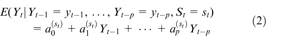
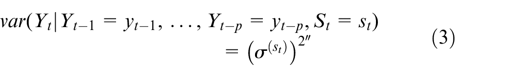
The conditional distribution of
The conditional distribution of
The standardised AR(p) model with Gaussian innovations, where

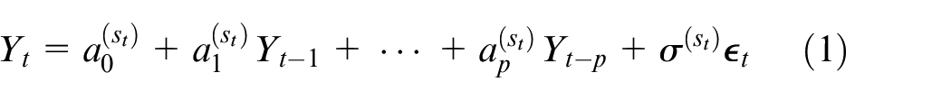
METIS uses the EM to fit the MS-AR model for the prescribed values

where
A Viterbi algorithm is used in the METIS toolbox to provide a visual representation of the path of the hidden states, and the plot indicates which AR weather regime is most likely, given the observation time as shown in Figure 2. This plot was produced for model with six lags and three hidden states for the December at the UK North East location. In this plot, the allocation of the first weather type or regime is denoted by the solid line, regime two by the dashed line and regime three with the dotted line. An accompanying table listing the parameters of the AR model operating in each hidden state is also included in Figure 2. In regime two, the wind speed demonstrates greatest variability, whereas in regime one, the wind speed appears to change much slower, as confirmed by the values for
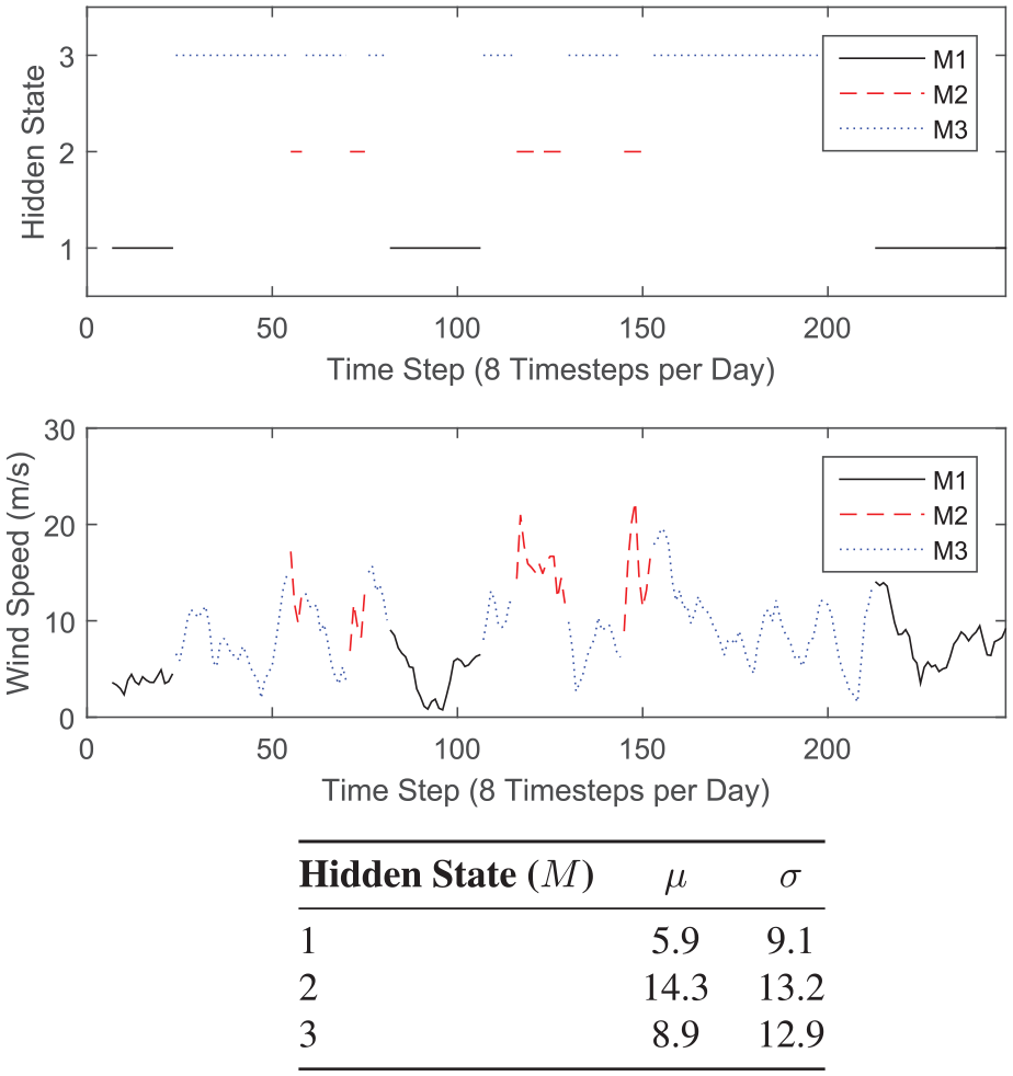
Resulting Viterbi algorithm from homogeneous MS-AR Gaussian model for wind speed, 3-h time steps, 34 years, UK North East,
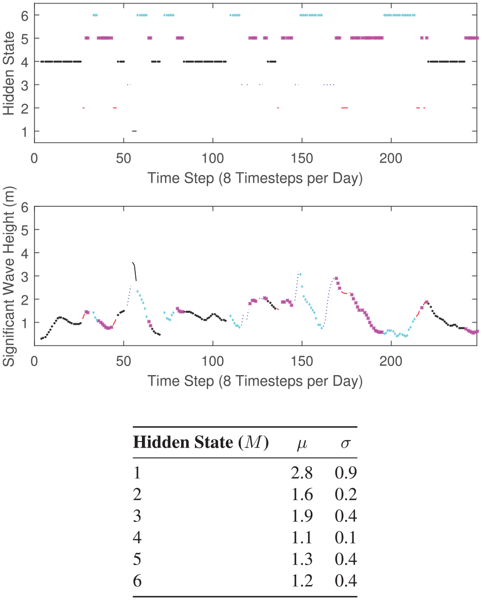
Resulting Viterbi algorithm from homogeneous MS-AR Gaussian model for significant wave height, 3-h time steps, 34 years, UK North East,
Wave heights are directly affected by wind speed, the length of time the wind blows and fetch, which is the distance on the water surface the wind blows. This means that during periods of low wind speed, the waves will be small, irrespective of wind duration or fetch. If wind speeds are high for a short period even with a large fetch, the waves will remain low. For high wind speeds over a short fetch, the wave heights are still low. It is only when these three conditions combine those large waves will form. It seems that these forces may be apparent in Figures 2 and 3, where higher wave heights are noticeable in Figure 2 at time steps shortly after higher and prolonged wind speeds in Figure 3.
The MS-AR model can then produce the defined number of monthly sets through simulation. The simulation function simulates the AR process with Markovian switching, which are dictated by the hidden Markov chain. This computation uses the path of the hidden Markov variable, identified as part of the Viterbi algorithm and the parameters of the AR models. The matrix of the initial observations is used to define the output dimension of the simulated instances.
Model selection
In order to identify the best model for

To understand the number of previous values or lags that are statistically significant for the AR part of the MS-AR model, the monthly data of all three locations in Table 1 were assessed in terms of the autocorrelation function (ACF) and partial autocorrelation function (PACF). The PACF can be used to define the partial correlation of a time series against its own lagged values. The purpose of this approach was to try and identify a ceiling for the AR model order and therefore constrain the maximum number of model types to be considered in the BIC assessment process. The ACF included in Figure 4 shows a fast geometrical decline, which is representative of stationary processes and that an AR model is suitable to describe the data. Moreover, the PACF shows that up to as many as six lags are statistically significant for the AR model prediction. It should be noted that the example shown in Figure 4 is taken from the UK North East data set and that the month of March was one of few months to demonstrate the dependence of up to six lags, which for three hourly samples corresponds up to 18 h in the past. The same process was followed for significant wave height, and it was identified that up to three lags were statistically significant.
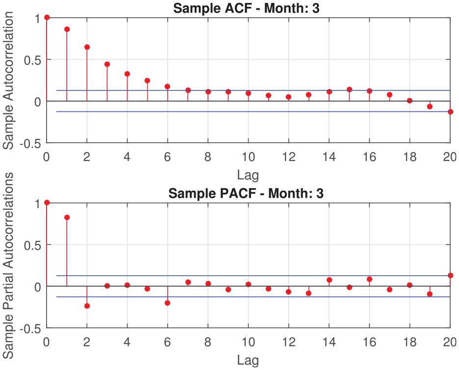
Sample autocorrelation (ACF) and partial autocorrelation (PACF) correlograms –
Once a ceiling value for the AR model order is identified, the process of checking the MS-AR model types can be completed. This involves running the EM algorithm in the METIS toolbox to obtain the parameters
It is time expensive to run the EM algorithm for all of the model types each time a new observed weather series is to be assessed. Therefore, a review of the model types selected across the three sites was completed and the results are shown in Figures 5 and 6. It is shown that for the wind speed
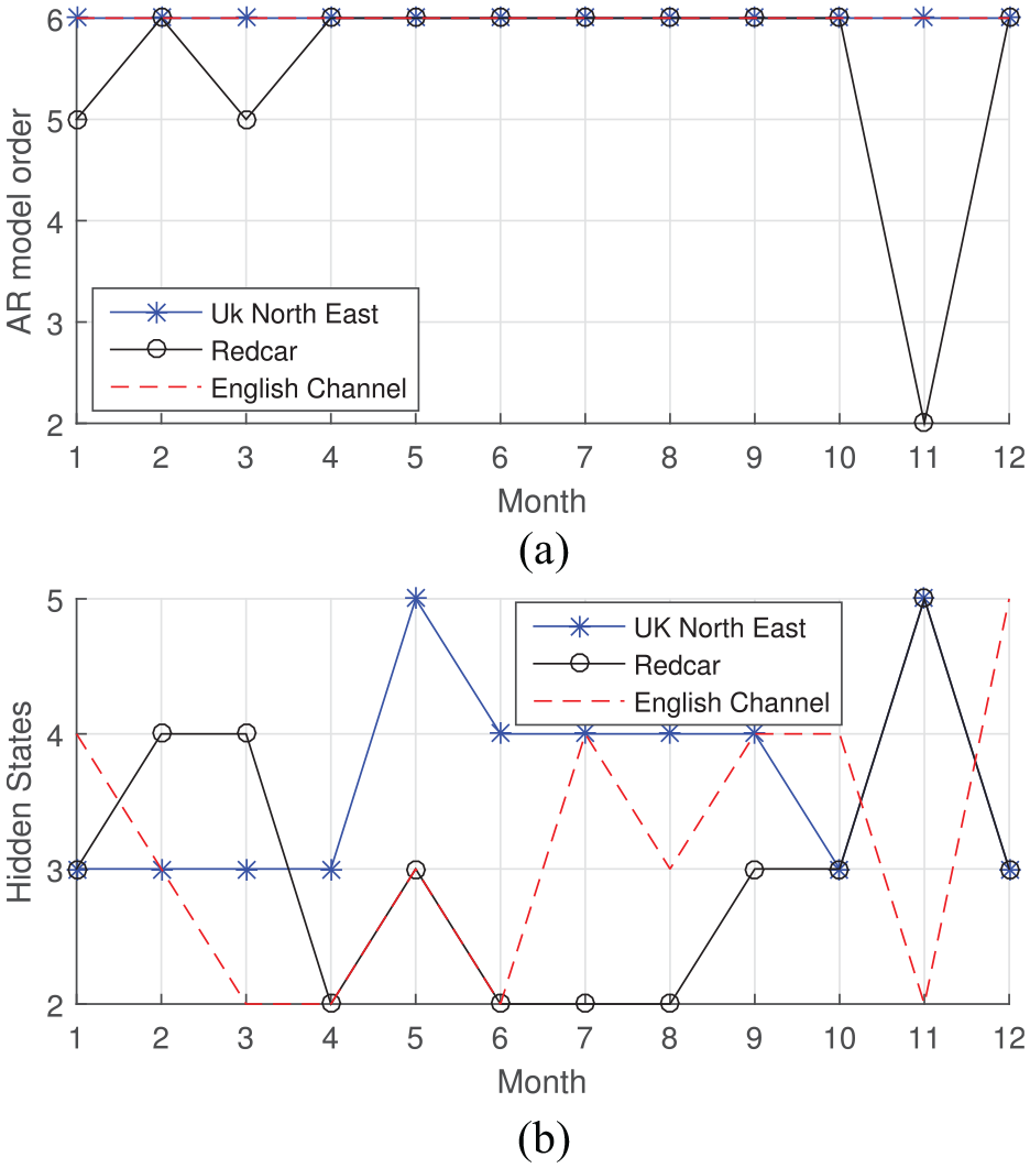
Wind speed MS-AR model selection: (a) AR model order p and (b) hidden states M.
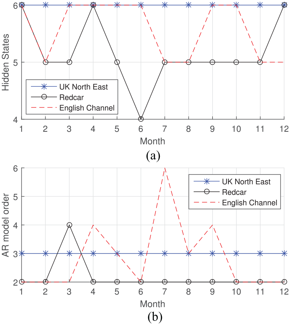
Significant wave height MS-AR model selection: (a) AR model order p and (b) hidden states M.
Simulation and time series composition
Once the most suitable model for each month and meteorological parameter is identified, the simulation process can be summarised as follows:
The EM algorithm is run once again for each month based on the value for
For each simulation (normally 1000), the estimated parameters from the EM algorithm are then used to simulate one instance of the Markov chain, which allocates the hidden states to each time step and thus the allocation of each AR model across the time series.
This distribution of hidden states is then carried into the AR simulation. The AR simulation takes a random year of observations for the given month, which provides a reference for the first set of previous values corresponding with the model order
This process continues following the path of the hidden states until a new time series is produced. The process is repeated for each month for as many simulations specified by the user, resulting in variable time series realisations, stemming from a combination of independent state allocations, random selection of observed data and the AR computation.
After the simulations are completed, multiple realisations of each month for
Results
Simulation results
In this section, we begin with the visual and numerical outputs from the presented methodology. Table 2 compares the mean metocean values across all three sites. The mean values for the observed and simulated data have not been included, and instead the percentage difference is listed to convey the variation between the observed and modelled data.
Percentage difference, average and absolute average error for wind speed
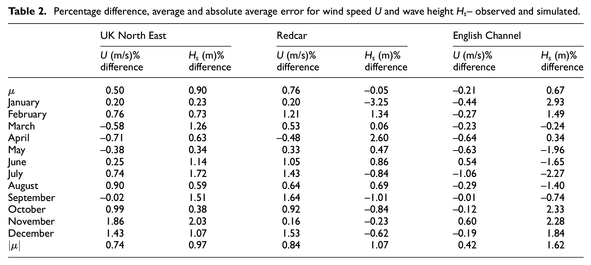
It is shown that the MS-AR model tuned to each site and month is capable of following the seasonal changes in the observed series, with the majority of errors below 2%. Generally, the models were found to have larger average values for
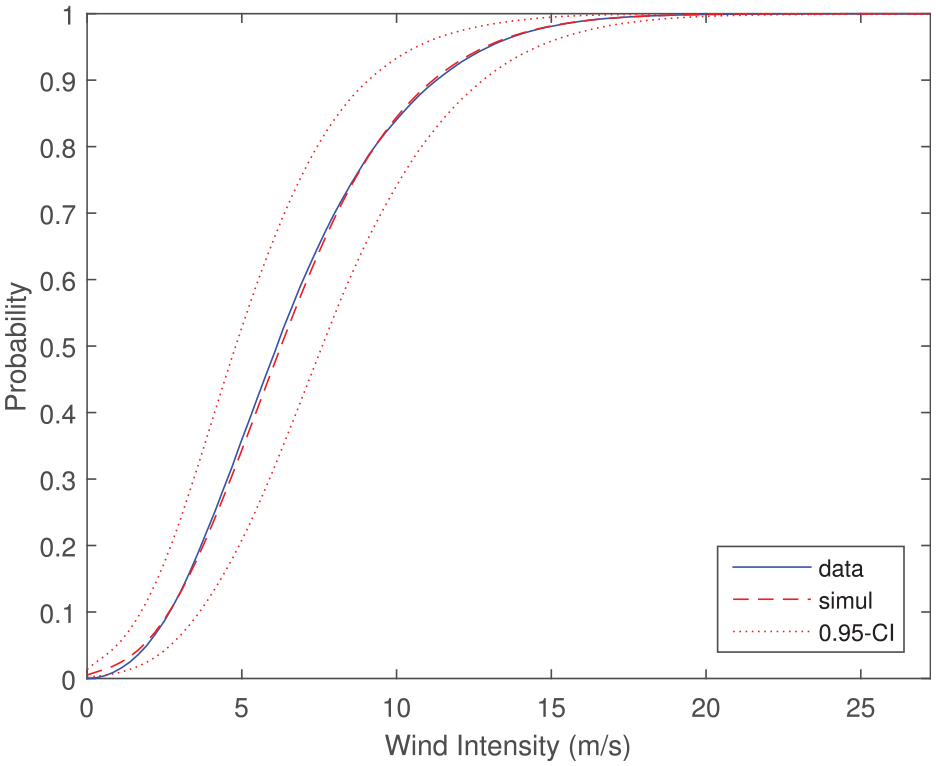
Comparisons for the UK North East site are used in the following to summarise the typical outcomes of the analysis. In Figures 7 and 8, the CDFs are shown for the wind speed and wave height, respectively. Each figure represents the distribution of
CDFs of annual wind speed – observed versus simulated – UK North East.
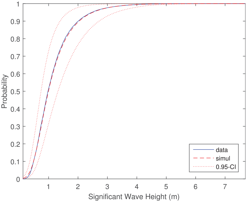
CDFs of annual wave height – observed versus simulated – UK North East.
It is evident in Figures 7 and 8 that the CDF of the simulated data follows the observed years of annual data. Looking at the lower wind speeds and wave heights in both figures shows that there is a tendency for the model to over predict the occurrence of
An additional visual inspection uses a quantile–quantile plot (QQ plot) of the annual observed and simulated time series. This tests if the simulated outcomes are related to the same distribution as the observed data. The QQ plots for
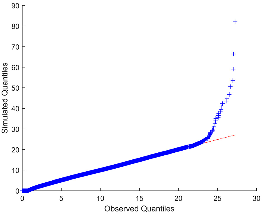
QQ plot: observed and simulated wind speed – UK North East.
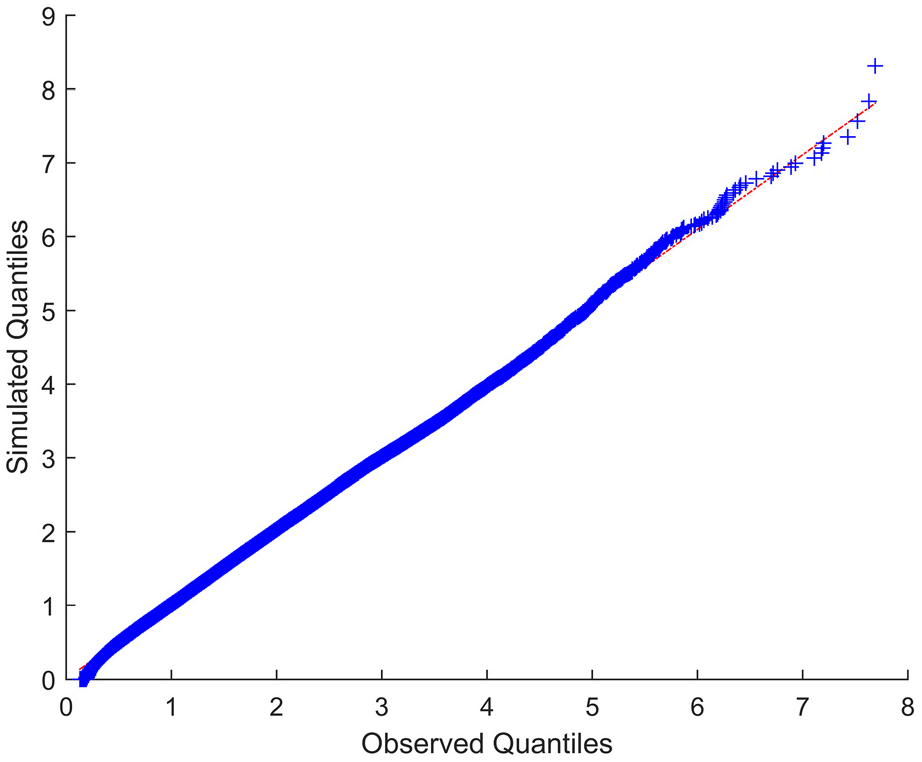
QQ plot: observed and simulated wave height – UK North East.
Weather window assessment
This section presents the results for a weather window assessment across all three sites investigated. By considering a typically constrained offshore task against the simulated data series, the suitability of the employed methodology and generated time series can be reviewed.
For this assessment, specified weather limits and duration for a personnel transfer operation were applied against the three data sets, which are summarised in Table 3. This type of task is regularly completed during offshore wind installation, particularly when personnel are transferred to transition pieces for turbine installation. Similar tasks are also completed regularly in other marine sectors and therefore presents a relevant case study. A weather window can be defined simply as weather conditions that are less than or equal to the environmental limits of a task for a period of time. In some instances, a fixed periods less than or equal the environmental limits are specified for the weather window criteria. These predefined window lengths are often applied in offshore planning to account for uncertainties in weather forecasting, ensuring that suitable contingencies are included that allow safe completion of the marine operations.
Weather window requirements.
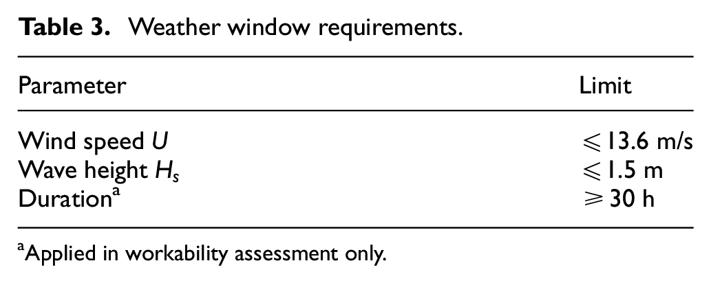
Applied in workability assessment only.
Weather window persistence and lengths
To demonstrate the application of the MS-AR model, we present a case study on a personnel transfer task from a CTV to a pre-installed turbine transition piece, which is constrained by specified working limits, described in Table 3. We begin with an assessment for weather window persistence and average window length, which considers only the wave height and wind speed parameters. This is applied to assess the characteristics of the simulated and observed data without considering a constraint for a minimum weather window duration.
In Figure 11−13, we show the weather window persistence and average window length for each location. The weather window persistence is presented as normalised frequencies of 10-h bins and for all three sites, the same clustering towards the lower bin values between 10 and 40 h is observed. The comparison of the observed and simulated data shows reasonable consistency with the largest differences shown for the English Channel. It is apparent that the simulations have a tendency to over predict the frequency of weather windows between 20- and 100-h bins, particularly for UK North East and the English Channel, while Redcar shows the closest comparison overall. The general outcome of persistence histograms shows little difference between the observed and simulated data, which indicates that the modelled time series captures the characteristics at each site.
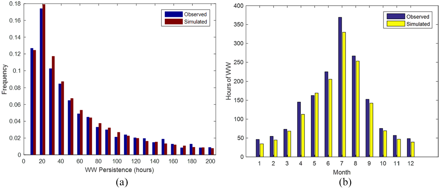
UK North East – weather window persistence histogram and average window length –≤13.6 m/s and ≤1.5 m: (a) weather window persistence – 10-h bins – UK North East and (b) average weather window duration – UK North East.
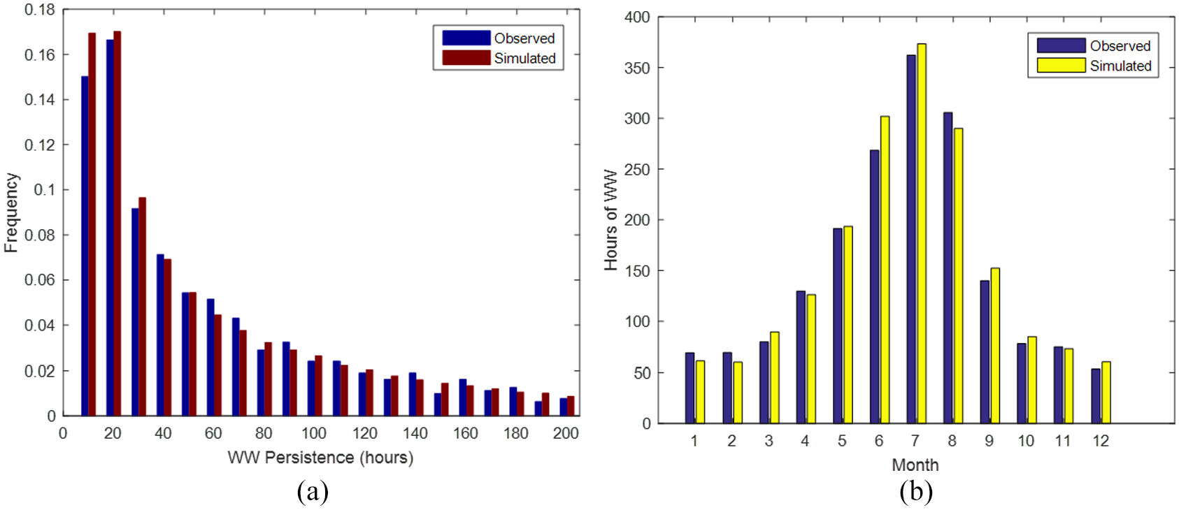
Redcar – weather window persistence histogram and average window length –≤13.6 m/s and ≤1.5 m: (a) weather window persistence – 10-h bins – Redcar and (b) average weather window duration – Redcar.
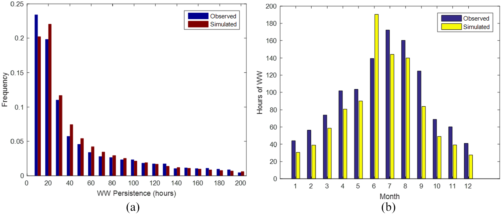
English Channel – weather window persistence histogram and average window length –≤13.6 m/s and ≤1.5 m: (a) weather window persistence – 10-h bins – English Channel and (b) average weather window duration – English Channel.
The average weather window length for each month and location are shown in Figures 11(b), 12(b) and 13(b). The largest difference is again seen for the English Channel, which demonstrates that the modelled data generally produce smaller weather windows for each month by approximately 10–20 h. A similar outcome is shown for UK North East, but with smaller average differences. Redcar again shows the closest outcome for the average window length with no predominant over or under prediction identified. The outcomes for UK North East and the English Channel suggest that some difference could be expected when simulating the progression of marine operations against the modelled data, which we will review in the following section.
Average monthly workability
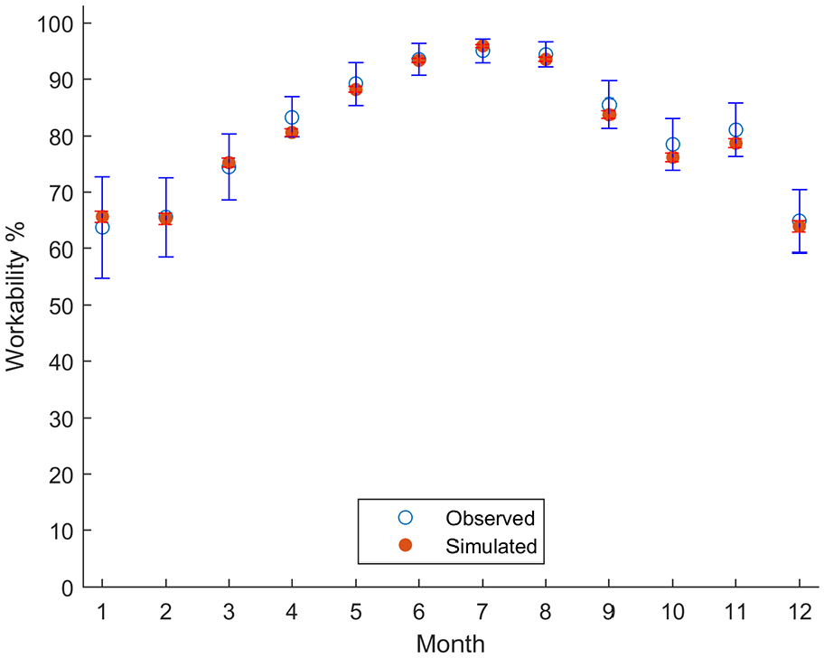
In this section, we consider an assessment of all limitations included in Table 3. This is completed to extend the weather window assessment for a predefined duration of more than or equal to 30 h. This duration constraint is introduced to assess the modelled time series with a realistic condition that may be applied to an operation from marine warranty surveyors or planning personnel. This assessment considers the average percentage workability of the personnel transfer operation, which considers the average amount of time available to complete the operation for each month and location, above or equal to the 30-h threshold. In Figures 14−16, we show scatter plots for the workability across the three sites.

Mean percentage workability for time ≥30 h at ≤13.6 m/s and ≤1.5 m – UK North East.
Mean percentage workability for time ≥30 h at ≤13.6 m/s and ≤1.5 m – Redcar.
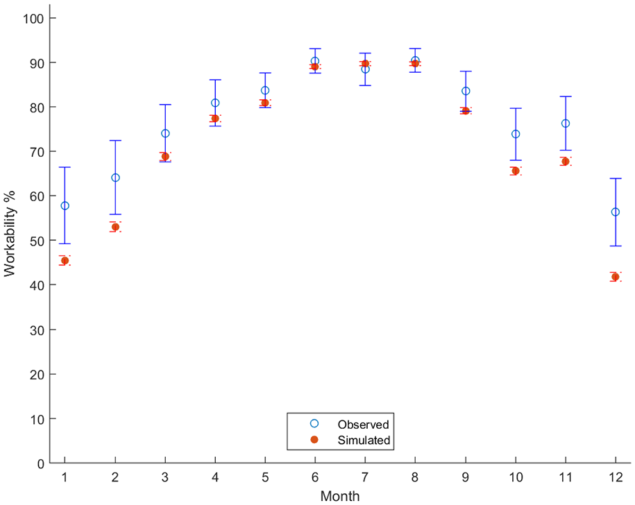
Mean percentage workability for time ≥30 h at ≤13.6 m/s and ≤1.5 m – English Channel.
In Figures 14−16, error bars are included for a 90% confidence interval from the observed and simulated data sets. The site with the closest percentage workability was Redcar with the largest variations observed for January, July and March. Overall the modelled data were found to have 1.5% more workability on average when compared to the observed data set. The next closest prediction was identified at UK North East at approximately 3% less workability on average with the modelled data showing larger variations in the winter months, with the largest recorded at 9.8% less workability for February. The English Channel site reveals considerable deviations, and the workability of the simulated outcomes was found to exhibit 7.2% less workability on average. Particularly, large deviations are observed for the winter months, most notably December, January and February at approximately 25%, 21% and 16%, respectively.
Overall, Figures 14−16 show that the simulated data have a tendency to under predict the workability in the winter months and over predict in the summer months. The under predictions in the winter months are much greater than the over predictions in each case, and the absolute percentage difference for UK North East, Redcar and the English Channel was found to be 3.5%, 1.9% and 8.9%, respectively. The 90% error bars show that the mean outcomes for the simulated data are within the range of the observed data sets across all months for UK North East and Redcar. In Figure 16, it is shown that the mean outcome lies outside the 90% confidence interval for January, February, October, November and December.
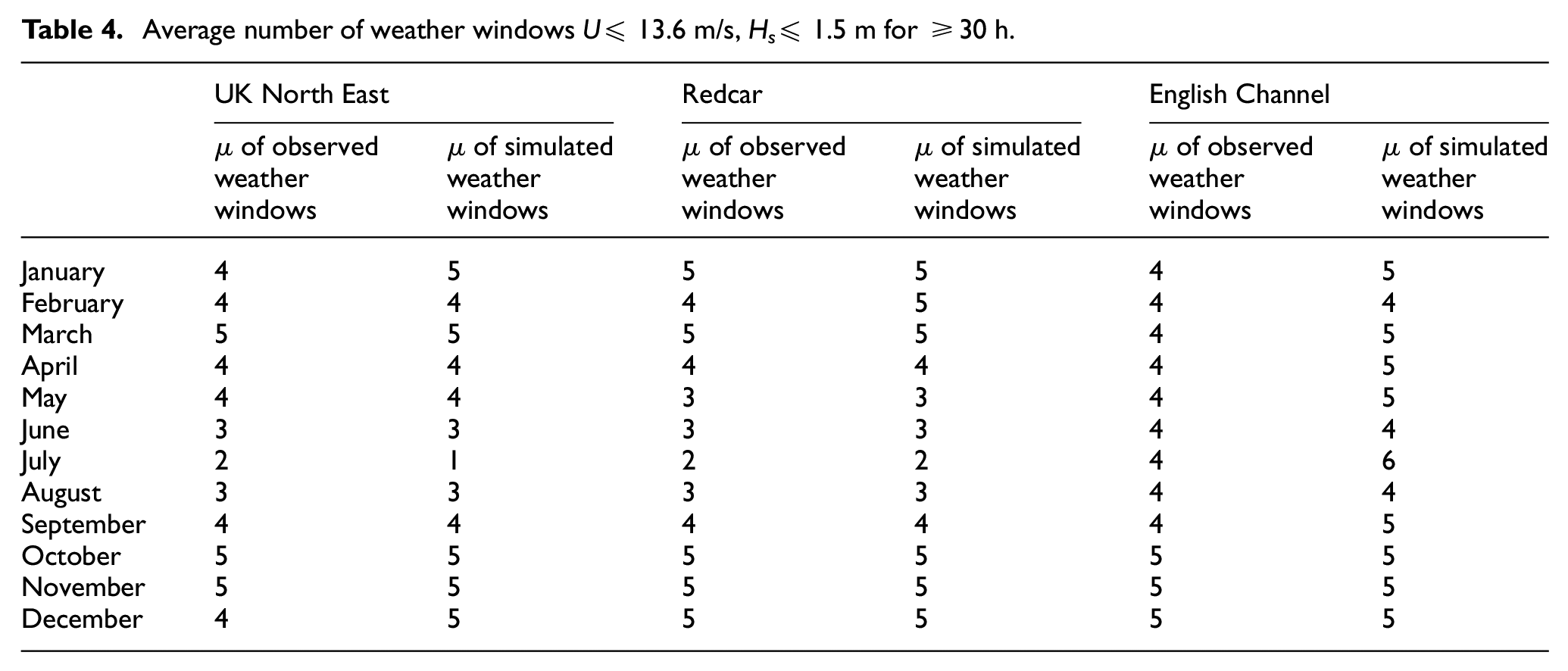
To produce a further perspective on these results, the average number of weather windows in each month was analysed for the three sites as shown in Table 4. Both Redcar and UK North East show very similar outcomes between the observed and simulated data indicating realistic working durations would be predicted using the simulated data. However, the English Channel showed the largest absolute percentage difference. On average, the modelled data exhibit more windows for the first 6–7 months. It should be noted that this does not necessarily mean more workability in the simulated data and is more likely due to the fragmentation of weather windows, which are believed to be less prominent in the observed data. Nevertheless, this outcome shows that despite the larger deviations in the winter months, there would likely be a similar amount of time to complete the required marine operations in each month. However, if the English Channel time series were comprised within a dedicated planning and simulation tool, it is likely the modelled data set would exhibit an increase in waiting times or more frequent interruptions, than the observed data set.
Average number of weather windows U≤ 13.6 m/s, Hs≤ 1.5 m for ≥30 h.
Correlated pairing method
The plots in the previous section showed significant deviations for the winter months, particularly for the English Channel location. It was originally suspected that the complex relationship between the wind and waves within an enclosed passage might have introduced a sensitivity to the methodology. However, a further review found that in many cases the wave time series contrasted against the wind pattern, which when used in a logistical simulation package, may lead to significantly conservative estimates for the progression of marine operations
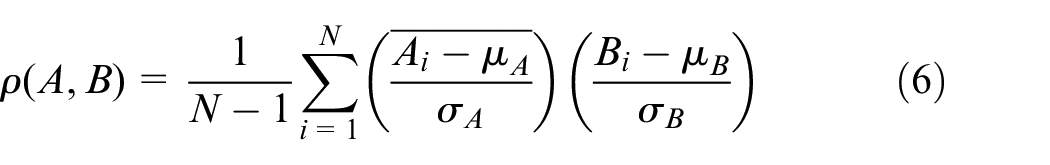
where:
To assess the severity of this mismatch between the simulated wind speed and wave height time series, the correlation between both parameters was investigated using the Pearson r correlation coefficient. The expression to define the Pearson r correlation coefficient or ‘Pearson r’ is listed in equation (6). The Pearson r between the wind speed at 10 m and Hs for the English Channel location was found to be 0.9. A review of the wind and wave correlations was completed for simulated English Channel data for the paired by means method, which resulted in a Pearson r of around 0.06.
It was not expected that the simulated data would be a perfect meteorological replication of the relationship between the wind and the waves; however, such a low coefficient did question the overall robustness of the weather model when compared to the correlation coefficient of the observed data for the English Channel. To improve this relationship, a second approach, which uses Pearson r coefficients to pair the wind and wave time series, was investigated. In this process, each monthly wind speed and wave height realisation were compared using the Pearson r correlation coefficient. For each wind speed realisation, the wave height with the largest Pearson r was selected for pairing. This resulted in the selection of a number of duplicate wave height series, which removed some unique realisations from the final composition. However, this approach was found to significantly improve the outputs for all months at the English Channel site, as shown in Figure 17. Once paired, the time series were again expanded to hourly time steps using linear interpolation.
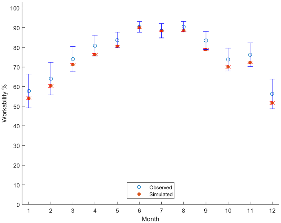
Mean percentage workability for time ≥30 h at ≤13.6 m/s and ≤1.5 m – English Channel – correlated pairing.
It should be noted that the final Pearson r for the simulated time series was around 0.5, which was 0.4 lower than the observed series for the English Channel. The final composition had approximately 4% less workability on average overall across the 12 months. When compared to the mean pairing approach, this is an increase of 4% workability on average. Notably large increases in workability were calculated for January, February and December compared to the first pairing method, increasing by approximately 15%, 12% and 17%, respectively. A reduction in workability is observed for April and August by 1% and 3%, respectively. A comparison of the average workability plots in Figures 16 and 17 shows that the data in correlated pairing approach fall well within the 90% confidence error bars of the observed outcomes, indicating a considerable increase in similarity between the two data sets. This result demonstrated a significant improvement using the correlation pairing approach for a site with a strong correlation between wind speed and wave height, which provides more flexibility to the modelling methodology overall.
Discussion
In this article, a methodology to produce annual time series of wind speed (
The authors were particularly interested in a dynamic metocean model that could be adapted to any location and select the best model types for each month. The MS-AR model developed by Monbet and Ailliot 7 can be applied to monthly data using a dedicated model in each instance, to produce monthly outcomes with similar characteristics to observed time series. The MS-AR model addresses the inadequacy of using a single AR model to describe the evolution of weather parameters, and in each month, it applies numerous AR models that operate within defined weather regimes. To reduce the number of model types and subsequent number of simulations, it is proposed that a future assessment could segment the data into seasonal sets and reviewed using the same methods in this article. This could determine if similar results are obtained within a reduced overall simulation time.
Ailliot and Monbet
9
have found that the BIC is a suitable method to select the best model order and number of hidden states to fit the data, despite acknowledging that this approach is not theoretically justified for MS-AR models. As such, an investigation using this assessment approach was presented and it was found that an envelope of model types was consistent across the three offshore sites for
The simulated outcomes for
In Figure 9, a right skew tail is shown, which indicates that some extreme wind speeds may have been produced in the simulation compared to the observed data set. However, the concentration of the points is quite low, especially for the most extreme points. Figure 10 shows a much slighter skew than was observed with the wind speed. This behaviour at the tails is expected to have little impact for marine planning applications as these extreme values are likely to span well beyond the operational constraints for these tasks.
To assess the validity of the overall methodology, the final annual compositions of
The workability plots presented in Figures 14−16 provide a further insight to on the characteristics of the simulated data by introducing a 30-h minimum threshold for the weather window limitations. The scatter plots have shown that the mean percentage workability of the simulated data falls within the 90% confidence interval for all months at each site with the exception of 4 months for the English Channel. The average number of weather windows was also reviewed for the same thresholds across the three sites, which revealed the fragmentation of the windows was fairly consistent with the observed data for UK North East and Redcar. The English Channel generally shows a larger number of weather windows in the simulated data, which indicates that more frequent delays or interruptions may be predicted using the generated time series. This gives a further indication that the simulated outcomes for the English Channel may lead to incorrect predictions if used for offshore planning and simulation applications. The observed data for the English Channel are shown to have the largest average wind speed for all three sites in Table 1, which may indicate the MS-AR model types considered have difficulty recreating data with larger excitations. However, when the values listed in Table 2 were reviewed, it was found that the largest absolute average percentage difference was recorded for the wave height simulations at the English Channel. Despite this outcome, the 1.62% difference is relatively small, which indicates that the cause of the differences exhibited in the weather window and workability plots may stem from elsewhere in the overall methodology.
The independently simulated
Conclusion
This article has presented a metocean modelling methodology using an MS-AR model with Gaussian innovations to produce stochastic wind speed and wave height time series for inclusion in marine risk planning tools. The METIS MATLAB toolbox developed by Monbet and Ailliot 7 provided the main simulation framework which was reconfigured to produce annual sets of wind and wave height data. The versatility of the MS-AR model for differing metocean regimes has been discussed, and we have implemented a BIC scoring process to select the most suitable model type for each weather parameter.
The MS-AR model was originally intended to produce wind speed outputs, yet it is demonstrated that realistic wave height simulations can be produced. Two approaches to pair the individual wind speed and wave height simulations have shown their validity to finalise the composition of simulated realisations. Some extreme and negative values were also identified in the simulated data sets. These instances were fairly infrequent and the negative values were subsequently replaced with zeros, while the extreme values are presumed to have a negligible impact as these values are far beyond the weather constraints considered for metocean planning.
Summarising statistics have been produced to compare the simulated and observed data against the weather limits of a personnel transfer operation. It is shown that the data for two out of three sites provide realistic predictions for the progression of this operation, indicating the suitably of the proposed modelling approach for metocean risk planning activities. An average percentage workability assessment is completed across the three sites, which demonstrates that the simulated data have consistently realistic characteristics for two locations using an initial pairing approach using mean values from each monthly realisation. The second correlated pairing technique showed an improvement in the workability percentages for the English Channel site, yet the simulated data were generally pessimistic overall. Both pairing methods are limited, and it is recommended that the overall methodology is used for sites with Pearson r correlations of ≤0.5 between the wind speed and wave height.
The constrained 90% confidence error bars for the simulated outcomes demonstrate that the modelling process can provide a means to pinpoint overall predictions, and would be suitable to calculate metrics such as exceedance probabilities that are commonly used to summarise marine risk profiles. It is concluded that the methodology presented will produce suitable wind speed and wave time series for the assessment of marine operations. It is recommended that the methodology is applied to other sites with strong correlations between wind speed and wave height, to determine the method’s adaptability to a wide range of offshore locations.
Footnotes
Acknowledgements
The authors would like to thank Monbet and Ailliot – Metocean Timeseries (METIS) Toolbox – 2005.
Declaration of conflicting interests
The author(s) declared no potential conflicts of interest with respect to the research, authorship, and/or publication of this article.
Funding
The author(s) disclosed receipt of the following financial support for the research, authorship, and/or publication of this article: This work is funded in part by the Energy Technologies Institute (ETI); Research Councils UK (RCUK); Energy programme for the Industrial Doctorate Centre for Offshore Renewable Energy (IDCORE) (grant number: EP/J500847/1).