Sage Journals: Discover world-class research

Abstract

Mate value is a construct that can be measured in various ways, ranging from complex but difficult-to-obtain ratings all the way to single-item self-report measures. Due to low sample sizes in previous studies, little is known about the relationship between mate value and demographic variables. In this article, we tested the Mate Value Scale, a relatively new, short, 4-item self-report measure in two large samples. In the first sample of over 1,000, mostly college-age participants, the scale was found to be reliable and correlated with criterion variables in expected ways. In the second, larger sample, which included over 21,000 participants, we have tested for differences across demographics. Contrary to theoretical expectations and previous findings with smaller samples, the differences were either very small (sexual orientation, age, education) or small (sex, socioeconomic status, relationship status) in terms of their effect size. This suggests that the scale is not measuring “objective” mate value (as understood either in terms of fitness or actual mating decisions by potential partners on the “market”), but a self-perception of it, open to social comparison, relative standards, possibly even biases, raising questions about measuring self-perceived versus objective mate value.

Keywords

mate value demographics self-perception psychometrics mate preferences

Research is often portrayed like a process of construction, where your carefully laid plans and purposeful efforts result in a neat, well-organized structure. Research, however, can also be similar to a journey when you do not necessarily end up where you planned to be. This article is a story of such a journey. We set out to simply validate a measure of mate value and test its relationship with demographics but ended up with unexpected results and perhaps more questions than answers.

Mate value and the perception thereof are practically unavoidable concepts in evolutionary psychology. If human beings, in the course of evolution, were selected to find “good” partners to enhance their reproductive fitness, then this implies that potential partners can be assigned different “values,” and the self can also be assigned such a “value” to save time and energy by not trying to get access to potential mates who would reject one anyway. Similarly, mating someone without detecting his or her low mating potential can be the costliest mistake both in the proximate and ultimate perspective (Jonason, Garcia, Webster, Li, & Fisher, 2015).

Thus, it is no wonder that over the past several decades, there has been a lot of theorizing on the “mate value” (e.g., Buss, 1989, Symons, 1985; and later, for instance, Brase & Guy, 2004; Buss & Shackelford, 1997; Edlund & Sagarin, 2010; Fisher, Cox, Bennett, & Gavric, 2008; Regan, 1998; Singh, 2002). All this research seems to share four underlying assumptions, namely, (1) individuals differ with respect to their value as potential mates on the “mating market,” (2) this value is assessed by their potential mates, (3) individuals have a by and large accurate sense of how much they are “worth” as potential romantic partners, and (4) the preferences driving these assessments were shaped by fitness and parental investment concerns over the course of evolution, that is, how to choose a mate who provides good genes or high parental investment or both to one’s offspring.

This concept of mate value may be difficult to measure, mainly due to the complexity of the variables involved and the cost of measuring some of them (for a short overview, see Edlund & Sagarin, 2014, pp. 72–73). Moreover, it can be measured either along distinct factors (e.g., Fisher et al., 2008) or holistically (e.g., Edlund & Sagarin, 2014). One may want to answer several further questions before measuring mate value. Along what dimensions do people evaluate themselves as potential partners? Are these dimensions the same as the ones they use to evaluate others (cf. Csajbók & Berkics, 2017; Fletcher, Simpson, Thomas, & Giles, 1999)? How are these dimensions combined to form up an “overall mate value?” Do people simply add up (or average) their evaluations or do they use some kind of weighting? Do they consider low evaluations along some dimensions to be “dealbreakers” (Jonason et al., 2015) or can these be compensated for by excelling in other traits? How do interactions on the mating market affect perceptions of one’s own mate value as well that of others?

One, apparently easy and practical way to overcome all these challenges is to accept a seemingly plausible assumption and simply ask people to assess their own mate value. If Assumption 3 is true, that is, people by and large know their own mate value (even without necessarily being aware of the underlying processes; Brase & Guy, 2004; Edlund & Sagarin, 2014), then, from a measurement perspective, all the complexities of mate value can be left for further research, and the researcher wanting to use mate value as a variable can proceed with a simple instrument. Finally, a brief and simple scale can easily be transformed so as to evaluate different targets (e.g., self, partner), and its briefness and simplicity reduce participant fatigue during administration of extensive test batteries (Gillen, Collisson, Murtagh, Browne, & McCutcheon, 2016).

Using this approach, one may go even as far as to assess mate value with a single item (Brase & Guy, 2004). Recently, a Mate Value Scale (MVS) was developed by Edlund and Sagarin (2014) along the same lines, but in order to increase reliability, it includes 4 items instead of just 1. Studies that used this scale report excellent internal consistency as measured by Cronbach’s αs, and this applies even to the partner’s mate value assessment (Blake, Bastian, O’Dean, & Denson, 2017; Brindley, McDonald, Welling, & Zeigler-Hill, 2018; Csajbók & Berkics, 2017; Edlund & Sagarin, 2014; Erik & Bhogal, 2016; Gillen et al., 2016; Kasumovic, Blake, Dixson, & Denson, 2015; Lemay & Wolf, 2016; March & Wagstaff, 2017; McDonald, Coleman, & Brindley, 2019). Evidence regarding the robustness of the MVS’s structure as assessed by confirmatory factor analysis (CFA) is, however, limited.

The research presented in this article started with the simple goals of testing the psychometric properties of the MVS and then by using novel and large samples, extending its validity and learning more about the relationship between mate value and demographics.

Mate Value and Self-Esteem

Self-perceived mate value and self-esteem are related constructs, as both of them involve an evaluation of the self. Manipulated rejections based on mating-specific attributes decreased self-esteem in both men and women (Pass, Lindenberg, & Park, 2010), and analogous results were achieved when individuals received derogatory comments regarding their mating-specific attributes (Campbell & Wilbur, 2009). Similarly, self-perceived mate value decreased when participants faced heterosexual rejection (Zhang, Liu, Li, & Ruan, 2015). Correlation between the global self-esteem and mate value in previous research varied according to how these variables were measured, from as low as r _male = .16, r _female = .26 (Shackelford, 2001), and r = .325 (Brase & Guy, 2004) to as high as r = .51 and .55 (Kirkpatrick, Waugh, Valencia, & Webster, 2002), r = .56 (Edlund & Sagarin, 2014), and r _male = .61 and r _female = .53 (Penke & Denissen, 2008). This may suggest that the global self-esteem and mate value can be concepts related yet distinct from one another (cf. Brown, 2006).

Mate Value and Demographics

Evolutionary psychology offers quite a few hypotheses about the relationship between demographics and mate value. Because men’s parental investment in terms of resources is essential at times when the mother cannot contribute due to caring for a child or children (Trivers, 1972), socioeconomic status (SES) should be more closely related to self-perceived mate value in men than in women. On the other hand, female appearance is an indicator of fertility, which is age-dependent, it is therefore expected that women’s age should be an important predictor of their mate value (Brase & Guy, 2004). Furthermore, it is predicted that being coupled is an indicator of being desired as a spouse (Brase & Guy, 2004), but since self-esteem and marital satisfaction are also related (Roberts & Donahue, 1994), one may expect that relationship satisfaction will have a moderating effect on any positive relation between relationship status and mate value (Brase & Guy, 2004). Unfortunately, only a very limited amount of research exists on the demographics of mate value. The few studies that were published by and large support these evolutionary predictions (with respect to SES: Mafra & Lopes, 2014; sex and culture: Goodwin et al., 2012; sex, age, and marital status: Brase & Guy, 2004). On the other hand, although these studies both theoretically and empirically support the assumption of a relation between demographic variables and mate value, the robustness of their findings should be considered with caution due to small and special samples. Brase and Guy (2004) had a UK university campus sample of 155 participants, divided into as many as 12 cells in a 2 × 2 × 3 analysis of variance (ANOVA). Goodwin et al. (2012) had a large sample, but from seven different countries, making the sample size per country between 85 and 198, and all participants were students. Mafra and Lopes (2014) had a sample of 64 undergraduate students compared with 86 public school students. Thus, although the studies above are important because they seem to be the first and thus far only ventures to explore the demographics of mate value, their results were based on small samples of mainly students, limiting their external validity.

Self-perceived mate value is important in choosing a partner because people tend to adjust their preferences to their self-perceived mate value (Edlund & Sagarin, 2010; Regan, 1998; Wenzel & Emerson, 2009). As a consequence, people may apply positive assortment with respect to self-perceived mate value and self-evaluation of the partner (cf. Luo, 2017). Self-perceived mate value is therefore expected to correlate positively with expectations about a potential partner. The strength of these relations may, however, vary across the measured dimensions and may differ in men and women (cf. Csajbók & Berkics, 2017).

Goals and Presentation of the Studies

The aim of the current research was 2-fold: first, to test the MVS as a conveniently short measure of mate value against several measures of other, more or less related constructs (Study 1). Other measures of mate value were not included, as the MVS was already tested against the Mate Value Inventory (Kirsner, Figueredo, & Jacobs, 2003) and the Mate Value Single Item Scale (Brase & Guy, 2004) in the debuting research on the scale (Edlund & Sagarin, 2014). Additionally, in a previous study (Csajbók & Berkics, 2017), in a large sample of 2,179 participants, we have already obtained moderate to high positive correlations between MVS scores and self-ratings of mating-relevant traits (the correlations were especially high with self-ratings of physical attractiveness, .65 and .69 for females and males, respectively).

The second goal was to use the MVS to test for mate value differences across demographics in an unprecedentedly large sample (Study 2). To give a stronger emphasis to our findings regarding the demographics, many of the psychometric details, especially from Study 1, are moved to the Supplementary Material, and only the essentials are presented here.

Study 1

Convergent and discriminant validity of the MVS was tested by CFA in a large Hungarian sample, whereby self-esteem, life satisfaction, loneliness, and sociosexual orientation were employed as criterion variables. Since self-perception of mate value and self-esteem both involve an evaluation of the self, and thus can be related constructs, and also because previous research, too, has shown them to be correlated, it was expected that these two variables should correlate substantially but not so closely as to suggest that they are one single construct (cf. Brown, 2006, where it is suggested that discriminant validity is poor when r > .80). Correlation with mate value was expected to be moderate in the case of life satisfaction and loneliness, because these factors are conceptually less strongly related to mate value. Although mate value may be an important predictor (as well as a consequence) of life satisfaction and loneliness, these two factors may have other correlates as well, buffering against the link between mate value and them. For instance, a person with low mate value may have many friends or enjoy professional success and therefore score high on satisfaction and low on loneliness. For sociosexual orientation, expectations may be a bit more complex, as this construct consists of three distinct factors: desire for causal relationships, attitudes about them, and behavior (engaging in casual sex). For the former two, weak correlations were expected, because attitudes about and desire for casual sex may still be high in people with a relatively low mate value. For behavior, the correlations were expected to be positive, because for people with high mate value it is easier to attract casual partners, and high-value males may even adopt a more short-term strategy. However, as this link is more complex—also depending on how high (or low) people set their standards, what cultural values they have, and so on—the correlation is not expected to be as strong as with self-esteem.

Method

Participants and Procedure

A convenience sample of 1,131 heterosexual Hungarian adults (62.7% female) aged between 18 and 45 (M = 23.19, SD = 5.01) completed an online questionnaire using Google Forms platform. The questionnaire was advertised on social media. Participation was voluntary and anonymous.

Measures

The MVS (Edlund & Sagarin, 2014) was translated into Hungarian and back to English to check translation quality. The goal was to measure participants’ perceptions of their own mate value (see also Csajbók & Berkics, 2017; for the Hungarian translation of the scale, see the Supplementary Material). The scale consists of 4 items (all measuring in a single direction), which are rated on an anchored Likert-type scale from 1 to 7. Internal consistency of the scale in our sample was good (α = .86). Criterion variables were measured with the Rosenberg Self-Esteem Scale (RSES; Rosenberg, 1965; Hungarian version: Sallay, Martos, Földvári, Szabó, & Ittzés, 2014), the Satisfaction With Life Scale (SWLS; Diener, Emmons, Larsen, & Griffin, 1985; Hungarian version: Martos, Sallay, Désfalvi, Szabó, & Ittzés, 2014), the short version of the UCLA Loneliness Scale (ULS; Peplau & Cutrona, 1980; Hungarian version: Bőthe et al., 2018), and the revised Sociosexual Orientation Inventory (SOI-R; Penke & Asendorpf, 2008; Hungarian version: Meskó, Láng, Kocsor, & Rózsa, 2012). All of the above listed criterion measures had at least good (α > .80) internal consistencies in our sample.

Data Analysis

First, only the four MVS items (Partial Model 1), then the MVS and the RSES items together (Partial Model 2), and finally all of the items of the instruments above (full model) were entered into CFA models of increasing complexity in Mplus Version 7 as indicators, whereas the measured constructs functioned as latent variables or factors on which their respective indicators loaded. The full model and its results are presented here; see the Supplementary Material for further details. In line with previous literature, the MVS, the SWLS, and the short version of the ULS were represented as single factors; the SOI-R as three factors; and the RSES with a bifactorial structure including a general self-esteem factor and two methodological factors for positive/negative item wording (see Figure 1; cf., Urbán, Szigeti, Kökönyei & Demetrovics, 2014). The SOI-R behavior factor was measured with just 2 items: Item 2 was omitted due to a strong interitem correlation (r > .80). The full model was first fitted to the whole sample, then measurement invariance was tested across sex. Due to the nonnormal distribution of some items, MLR estimator was used.

Figure 1.
Illustration of the Partial Models 1 and 2, and standardised loadings of the full model.

Results

The full model fit the data acceptably in the pooled sample and had scalar invariance across sex (Table 1) because the decrease in fit indices did not exceed the recommended cutoff values (Chen, 2007). As seen from Table 2, the latent variable for MVS had a medium to strong correlation with self-esteem, life satisfaction, and loneliness (in descending order) in both the male and female subsamples. Mate value had only weak, if any, correlations with sociosexual orientation, the strongest being the link between mate value and the behavioral factor of the SOI-R. The means of the latent variables differed between the sexes in self-esteem and two of the SOI-R factors: Males had a somewhat higher self-esteem (M = .159), a much more positive attitude about casual sex (M = .853), and a much higher level of desire for casual sex (M = .926; all male means are standardized values with female means set at zero). The two sexes did not differ significantly in the latent mean of the MVS items (male M = −.093).

Table 1.
Model Fit and Invariance of the full model.

Model χ² (df) CFI TLI RMSEA [90% CI] Δχ² (df) ΔCFI ΔTLI ΔRMSEA

Pooled 1,733.037 (529) .940 .933 .045 [.043, .047]

Configural 2,218.085 (1,058) .942 .935 .044 [.041, .147]

Metric (loadings) 2,293.237 (1,094) .940 .935 .044 [.042, .047] 75.169 (36) −.002 .000 .000

Scalar (intercepts) 2,514.515 (1,120) .930 .926 .047 [.044, .049] 230.646 (26) −.010 −.009 .003

Table 2.
Interfactor Correlations and Standardized Sex Differences of Means.

Measures 1. 2. 3. 4. 5. 6. 7. Std. Sex Diff.

1. MVS — .651* .513* −.391* .183* .164* −.022 −.093

2. RSES .631* — .671* −.605* .105* .104* −.121** .159*

3. SWLS .549* .688* — −.593* −.004 .063 −.181* −.029

4. Loneliness −.502* −.647* −.633* — −.064 .003 .300* −.116

5. SOI behavior .308* .209* .138 −.200* — .653* .355* .060

6. SOI attitude .123 .123 .040 −.016 .399* — .486* .853***

7. SOI desire −.103 −.140* −.121* .234* .105 .440* — .926***

Note: All variables are latent variables of the full scalar model tested in Mplus Version 7. Correlations in the female subsample are above the diagonal, correlations for males below it. MVS = Mate Value Scale; RSES = Rosenberg Self-Esteem Scale; SWLS = Satisfaction With Life Scale; SOI = Sociosexual Orientation Inventory. Std. sex diff. = standardized sex difference. Female means were standardized to zero, values in the table are standardized male means.

p < .05. p < .01. p < .001.

Discussion

Results of Study 1 suggest that the MVS is a reliable and valid measure of self-perceived mate value. It correlates strongly with general self-esteem but not as strongly as to suggest that the two variables measure the same phenomenon. The latent mean of the MVS also shows medium to strong correlations with life satisfaction and loneliness, and its correlation with sociosexual orientation is, as expected, rather weak for the attitude and desire factors, while significant but still not high for the behavioral factor.

Study 2

The goal of Study 2 was to test the association between various demographic characteristics and mate value. More specifically, we examined differences in mate value across age, sex, level of education, SES, relationship status, and sexual orientation.

Females were expected to have a higher self-perceived mate value than men. Females tend to have a larger parental investment, thus they are the more selective or demanding of the two sexes, while males as the less investing sex have lower standards and are more interested in having more partners and initiating sexual relationships (cf. Buss & Schmitt, 1993). This implies that for men, it should be a more common experience that they have to compete and put effort in finding partners and face the possibility of rejection and failure, while for women, it should be a more common experience that they are desired and sought-after as potential partners, even though many times by men whom they themselves do not prefer. Certainly, there is much more to self-perceived mate value than that, so the effect may be so small that a really large sample is needed to detect it. In fact, previous studies with smaller samples have not found a main effect by sex (Brase & Guy, 2004; Goodwin et al., 2012; Mafra & Lopes, 2014), but in a previous sample of 2,179 participants, we did find such an effect (Csajbók & Berkics, 2017).¹ Since in Study 2, we had an even larger sample (see below), we expected a weak but statistically significant difference to emerge.

Concerning age, we predicted that its effect is sex dependent. Since in women, mate value is more dependent on youthful appearance than in men, it is expected to decline with age. In contrast, mate value in men is more closely related to status achievement, a factor that shows a positive association with age. Mate value in men ought to be therefore either stable across different ages or even increase with age (see Brase & Guy, 2004). Similarly, we expected that sex and SES would show an interaction with respect to mate value, as well as sex and education, since the latter is an important predictor of social status. Previous studies suggest that men with higher status and education estimate their mate value higher, and in women, this relation is much weaker (Mafra & Lopes, 2014).

Finally, we tested the effect of relationship status on mate value. We expected that single participants would have lower self-perceived mate value for two reasons: (1) they may be single because of actually having a low mate value and evaluate their mate value in the light of their lack of success in mating and (2) they may temporarily assess their self-perceived mate value lower due to recent mating failures. However, this hypothesis may be qualified by the concern that some of the single participants might stay single to pursue more short-term affairs, thus having a more unrestricted sociosexuality. Additionally, we have seen in Study 1 that SOI’s behavioral aspect correlates positively with self-perceived mate value. Therefore, single participants were analyzed according to how many sexual partners they had. Further, in coupled participants, relationship satisfaction may also correlate with mate value. It has been shown that marital disharmony decreases self-esteem (Shackelford, 2001). One may therefore compare the self-perceived mate value of single participants to values found in persons unsatisfied with their existing relationships.

Method

Participants and Procedure

The participants were Hungarian adults (14,441 male, 6,847 female), aged between 18 and 76 (M = 33.45, SD = 11.29). Participants were recruited online on “444.hu,” a gonzo-type, politically leftist-liberal news portal popular among young, urban, educated readers. Thus, the sample was not representative of the Hungarian adult population, but it was large enough to include at least a few hundred participants from demographics that were underrepresented in it (e.g., people above 50, people with only a primary education, or people having below-average living conditions).

To enhance data reliability, participants were removed from the sample if their responses were largely incomplete or if they gave inconsistent responses (e.g., reporting that their first sexual encounter happened at an age they were younger than) or if they gave unengaged responses (e.g., they gave the same response to a number of questions including reverse items).

Based on their self-report, 17,978 (84.5%) participants viewed themselves as heterosexual, 1,932 (9.1%) as heterosexual with some same-sex attraction, 563 (2.6%) as bisexual, 140 (0.7%) as homosexual with some other-sex attraction, 511 (2.4%) as homosexual, 37 (0.2%) participants viewed themselves as asexual, and 127 (0.6%) were ambiguous as to their sexual orientation (the latter two groups were excluded from group comparisons due to small sample sizes). In total, 5,248 (24.7%) participants reported being single, 8,939 (42%) in a relationship, 851 (4%) engaged to be married, 5,233 (24.6%) married, 596 (2.8%) divorced, 104 (0.5%) widowed, and 317 (1.5%) reported other specific types of relationship. Again, the two last-named groups were excluded from group comparisons due to small sample sizes.

Of the participants, 59% reported higher education, 33.1% graduated from high school, 4.7% from vocational education, and 3.3% from elementary school. SES was assessed by a single item ranging from 1 (the worst living conditions) to 7 (the best living conditions). However, due to a low number of participants who indicated a low status, we decided to create subgroups in order to create sufficient sample sizes for comparison. In this way, we ended up with 4.8% participants who reported living in worse-than-average conditions, 25% in average living conditions, 43.4% somewhat better than average, and 26.8% better than average or best living conditions. With respect to the place of residence, 52.6% lived in the capital, 37.7% in cities and towns, and 9.6% in villages. In total, 68% of participants had no children and 3% had not yet had a sexual partner in their life.

Measures

Participants completed an online questionnaire implemented with the Qualtrics platform. They filled in the MVS, and if they were in a relationship, they also rated their general relationship satisfaction on a 5-point Likert-type scale. They were also asked to give the number of sexual partners they had (response options were exact numbers up to 10, and categories, e.g., “21–30” above 10).

Minimum long-term partner standards were assessed by a partner preference trait list adapted from Csajbók and Berkics (2017). This trait list consists of 23 items, loading on seven essential dimensions of partner evaluation. In the current study, participants were asked—independently of being currently in a relationship—to indicate the minimum level of each characteristic they would require in order to initiate a long-term relationship with a potential partner on a 7-point Likert-type scale (1 = not at all important that my partner should be like this, 7 = very important that my partner should be like this).

Data Analysis

First, only the 4 MVS items (simple model), and then the 4 MVS as well as the 23 minimum standards items (full model), were entered into CFA models in Mplus Version 7 as indicators. The measured constructs were latent variables or factors on which their respective indicators loaded: one factor for the MVS items, and seven factors for the minimum standards items. The seven factors of minimum standards were warmth, emotional stability, physical appearance, sexual passion, social status, intellect, and dominance (for details, see Csajbók & Berkics, 2017).

The psychometrics of Study 2 are presented in more detail, because invariance testing was necessary for comparisons across demographics. First, both models were fitted to the whole sample, then measurement invariance in the simple model was tested across the demographic variables used for comparisons. Invariance was first tested across sex and sexual orientations, then for heterosexual participants only, across age groups, education, SES, and relationship status. For the simple model (MVS only), ML estimator was used. Of the fit indices, CFI was considered to be the most important, because TLI and especially RMSEA are sensitive to model parsimony, imposing a penalty on models with a low df (see Brown, 2006, pp. 83–86), but the latter indices are also included for the sake of comparing configural, metric, and scalar models. Due to a nonnormal distribution of some of the minimum standards items, MLR estimator was used for the full model. In this model, invariance was tested across sex only, because the purpose of adding the minimum standards items was to analyze the MVS in a more complex model with better RMSEAs and to see if the MVS scores correlate positively with minimum standards as previous research has shown. In the full model, only heterosexual participants were included because in some of the nonheterosexual groups the sample sizes were low. The models are shown in Figure 2.

Figure 2.
Illustration of the Simple Model, and standardised loadings of the Full Model.

The effect of the various demographic variables (sexual orientation, education, SES, age, and relationship status) on the mean of the MVS was tested using two-way ANOVAs, with sex as the other independent variable, to compare categories of education, status, and age in a way similar to previous studies (Brase & Guy, 2004; Mafra & Lopes, 2014). Except for sexual orientation, demographic effects were tested in heterosexual participants only.

When testing for the effect of age—in order to detect a possible significant drop around menopause or other specific age categories—ranges were based on two considerations: (1) balancing the number of participants in each age group and (2) setting the ranges in meaningfully specific sections. The sample was therefore divided in eight groups based on cutoff points at 21, 26, 31, 36, 41, 46, and 51 years of age (see Table 3 for mate value results for both sexes and all age groups). Since sample sizes and variances in the different demographic groups in some cases differed significantly, Games–Howell type post hoc analysis was chosen. Although the results of the two-way ANOVAs are reported, for ease of interpretation, post hoc analyses are performed on the two sexes separately. Where possible, Pearson (for age) or Spearman (for education and SES) correlation was computed to test the linear relationship between mate value and interval or ordinal demographic variables.

Table 3.
Descriptive Statistics for Mate Value in Relation to Sex and Age.

Sex Age Groups (Years) N Mean SD

Male 18–20 733 4.86 1.16

21–25 2,341 4.76 1.14

26–30 2,316 4.76 1.10

31–35 1,818 4.72 1.08

36–40 1,756 4.72 1.07

41–45 1,453 4.71 1.01

46–50 927 4.64 0.97

Older than 51 1,439 4.62 0.93

Female 18–20 432 5.03 1.06

21–25 1,523 5.11 0.95

26–30 1,171 5.13 1.07

31–35 669 5.16 1.00

36–40 478 5.00 1.04

41–45 401 4.97 1.06

46–50 258 4.75 1.11

Older than 51 263 4.78 1.04

To estimate the overall predictive strength of the demographic variables for mate value, we ran two linear regression analyses, one for each sex. For SES, education, and relationship (combined with relationship satisfaction and number of sexual partners), we created dummy variables and chose their baseline according to the largest subgroups to avoid multicollinearity (somewhat better than average living conditions, high school education, and being in a good relationship for SES, level of education, and relationship status, respectively).

Results

Model Fit

The simple model with the 4 MVS items fits the data in the pooled sample well (see Table 4) with the exception of a poor RMSEA, which is, however, known to perform badly in very simple models (for a model consisting of four indicators loading on one factor, just like in our case, see Kenny, Kaniskan, & McCoach, 2015). Scalar invariance was established across all of the demographic variables, except SES, for which partial scalar invariance was established at the cost of relaxing the intercept of 1 item (see the Supplementary Material for details). The full model also had an acceptable fit to the data, although scalar equivalence across sex could only be partially established, by relaxing the intercept of an MVS and a minimum standards item.

Table 4.
Model Fit and Invariance in the Simple and the full model.

Model χ² (df) CFI TLI RMSEA [90% CI] Δχ² (df) ΔCFI ΔTLI ΔRMSEA

Simple model (Mate Value Scale [MVS] only)—equivalence across sex and sexual orientation

Pooled 922.086 (2) .982 .946 .148 [.140, .156]

Configural 962.848 (12) .981 .944 .150 [.142, .158]

Metric (loadings) 1,002.393 (27) .981 .974 .101 [.096, .107] 39.546(15) .000 .030 −.049

Scalar (intercepts) 1,423.163 (42) .973 .977 .097 [.092, .101] 420.770(15) −.008 .003 −.004

Simple model (MVS only)—equivalence across age groups

Configural 882.806 (16) .980 .941 .155 [.147, .164]

Metric (loadings) 944.837 (37) .980 .973 .104 [.099, .110] 62.041(21) .000 .032 −.041

Scalar (intercepts) 1,258.049 (58) .973 .978 .096 [.091, .101] 313.202(21) −.007 .005 −.008

Simple model (MVS only)—equivalence across education

Configural 805.963 (8) .982 .946 .149 [.140, .158]

Metric (loadings) 845.871 (17) .981 .973 .104 [.098, .110] 39.908(9) −.001 .027 −.045

Scalar (intercepts) 983.523 (26) .978 .980 .091 [.086, .095] 137.652(9) −.003 .007 −.013

Simple model (MVS only)—equivalence across socioeconomic status

Configural 747.382 (8) .982 .947 .143 [.135, .152]

Metric (loadings) 799.428 (17) .981 .974 .101 [.095, .107] 52.045(9) −.001 .027 −.042

Scalar (intercepts) 1,428.052 (26) .966 .969 .110 [.105, .114] 628.625(9) −.015 −.005 .009

Scalar (partial)^a 987.922 (25) .977 .976 .097 [.092, .102] 188.494(6) −.004 .002 −.004

Simple model (MVS only)—equivalence across relationship status

Configural 832.835 (12) .980 .941 .152 [.143, .161]

Metric (loadings) 925.701 (27) .979 .971 .106 [.100, .112] 92.866(15) −.001 .030 −.046

Scalar (intercepts) 1,057.489 (42) .976 .979 .090 [.086, .095] 131.788(15) −.003 .008 −.016

Full model (MVS and minimum standards scales)—equivalence across sex

Pooled 10,431.191 (296) .937 .925 .044 [.043, .044]

Configural 10,642.896 (592) .934 .922 .043 [.043, .044]

Metric (loadings) 10,946.087 (611) .933 .923 .043 [.043, .044] 306.605(19) −.001 .001 .000

Scalar (intercepts) 12,863.778 (630) .920 .911 .046 [.046, .047] 2,248.779(19) −.013 −.012 .003

Scalar (partial)^b 12,068.345 (628) .925 .917 .045 [.044, .046] 1,281.858(17) −.008 −.006 .002

^aPartial scalar invariance was assessed by relaxing the intercept of 1 item (MVS4).

^bPartial scalar invariance was assessed by relaxing the intercept of 2 items (MVS2 and “attractive”).

Correlations between the MVS and the minimum standards factors, as well as sex differences in these variables, can be found in Table 5. The two sexes were analyzed separately but the pattern was similar: The MVS correlated positively with the seven minimum standards dimensions, and in both sexes, the highest level of correlation was observed with passion and appearance.

Table 5.
Interfactor Correlations and Standardized Sex Differences of Means.

Latent factors 1. 2. 3. 4. 5. 6. 7. 8. Std. Sex Diff.

1. MVS — .145 .064 .290 .331 .185 .162 .209 0.287*

2. MS warmth .153 — .737 .178 .289 .160 .389 .495 0.850*

3. MS stability .022 .748 — .106 .158 .191 .247 .313 0.248*

4. MS appearance .347 .275 .161 — .454 .442 .187 .292 −1.039*

5. MS passion .342 .431 .304 .620 — .314 .247 .526 0.052*

6. MS status .132 .115 .181 .241 .247 — .233 .362 0.780*

7. MS intellect .193 .425 .281 .284 .304 .165 — .420 0.593*

8. MS dominance .183 .493 .418 .223 .469 .381 .483 — 1.200***

Note: All variables are latent variables of the full model tested in Mplus Version 7. Correlations in the female subsample are above the diagonal, correlations for males below. All correlations are significant at p < .001, except the one in italics (between MVS and minimum standards for warmth in the male sample), which is not significant. MS = minimum standards; MVS = Mate Value Scale. Std. sex diff. = standardized sex difference. Male means were standardized to zero, values in the table are standardized female means.

Mate Value Across Demographics

The average male mate value was 4.71 (SD = 1.08), while the average female mate value was 5.05 (SD = 1.05). This indicates a small but statistically significant difference in mate value between the sexes in the expected direction (i.e., females have higher mate value), t(13,846.60)= −22.20, p < .001, Cohen’s d = .32, R ² = .026. Highly similar results were achieved when only heterosexuals were tested: Females scored higher self-perceived mate value than men (M _male = 4.72, SD = 1.06; M _female = 5.06, SD = 1.03), t(17,976) = −19.343, p < .001, Cohen’s d = .33, R ² = .025.

Further analyses tested the effects of other demographic variables in 2 × 2 ANOVAs involving sex as the other independent variable. To test the effect of sexual orientation on self-perceived mate value, a two-way ANOVA was performed (across sex and sexual orientation; for the means and standard deviations, see Table 6). Results showed significant main effects of both sex, F _sex(1, 21114) = 48.727, p < .001, $η_{p}^{2}$ = .002, and sexual orientation, F _orientation(4, 21114) = 3.956, p = .003, $η_{p}^{2}$ = .001, and a significant interaction between sex (male or female) and sexual orientation, F _{sex × orientation}(4, 21114) = 5.265, p < .001, $η_{p}^{2}$ = .001. The Games–Howell post hoc test suggests that female mate value does not differ significantly across sexual orientation. Among male participants, on the other hand, hetero- and homosexual individuals scored higher self-perceived mate values than heterosexuals with some same-sex attraction.

Table 6.
Descriptive statistics for the Mate Value Scale Across Sex and Sexual Orientation.

Sex Sexual Orientation N Mean SD

Male Heterosexual 12,783 4.72 1.06

Heterosexual with some same-sex attraction 804 4.56 1.15

Bisexual 237 4.57 1.24

Homosexual with some opposite-sex attraction 99 4.49 1.23

Homosexual 445 4.76 1.14

Female Heterosexual 5,195 5.06 1.03

Heterosexual with some same-sex attraction 1,128 5.12 1.00

Bisexual 326 4.94 1.24

Homosexual with some opposite-sex attraction 41 4.93 1.06

Homosexual 66 4.89 0.99

After testing for the effects of sexual orientation, further analyses were performed on heterosexual participants only. Education had a significant main effect on mate value, F _education(3, 17970) = 13.483, p < .001, $η_{p}^{2}$ = .002, as also had sex, F _sex(1, 17970) = 108.103, p < .001, $η_{p}^{2}$ = .006. The interaction between these two factors was also significant, F _{sex × education}(3, 17970) = 3.681, p = .012, $η_{p}^{2}$ = .001, Spearman’s ρ was .088 for males (p < .001) and .026 for females (p = .056). For descriptive statistics, see Table 7. Games–Howell post hoc test had revealed that participants with only vocational or primary education had the lowest mate value among men, while high school graduates had higher, and college or university graduates had the highest self-perceived mate value. In women, education had no statistically significant effect on mate value.

Table 7.
Descriptive statistics for the Mate Value Scale Across Sex and Level of Education.

Sex Level of Education N Mean SD

Male Primary 380 4.61 1.22

Vocational 778 4.53 0.96

High school 4,172 4.64 1.09

Higher education 7,453 4.80 1.04

Female Primary 173 5.01 1.01

Vocational 116 4.99 1.00

High school 1,679 5.03 1.05

Higher education 3,227 5.08 1.02

SES had a significant main effect and interaction with sex on mate value, F _SES(3, 17970) = 322.447, p < .001, $η_{p}^{2}$ = .051; F _sex(1, 17970) = 235.824, p < .001, $η_{p}^{2}$ = .013; F _{SES × sex}(3, 17970) = 5.583, p = .001, $η_{p}^{2}$ = .001, Spearman’s ρ was .282 for males and .229 for females (p < .001 for both sexes). For descriptive statistics, see Table 8. Post hoc analyses suggest that SES affects self-perceived mate value systematically at all levels of status. In particular, the lower the individuals’ SES, the lower their self-perceived mate value. This holds for both sexes. Since Item 4 of the MVS had a problematic measurement invariance across SES, the two-way ANOVA was repeated on the mean of the first 3 items only. The results, however, including the post hoc analyses, showed the same pattern, F _SES(3, 17970) = 251.986, p < .001, $η_{p}^{2}$ = .040; F _sex(1, 17970) = 223.473, p < .001, $η_{p}^{2}$ = .012; F _{SES × sex}(3, 17970) = 3.237, p = .021, $η_{p}^{2}$ = .001.

Table 8.
Mean Results on the Mate Value Scale Across Sex and Socioeconomic Status (SES).

Sex SES N Mean of 4 Items SD of 4 Items Mean of 3 Items SD of 3 Items

Male Lower than average 632 3.97 1.23 3.86 1.29

Average 2,926 4.42 1.04 4.31 1.11

Somewhat better than average 5,614 4.73 1.02 4.59 1.10

Better than average 3,611 5.10 0.98 4.93 1.06

Female Lower than average 203 4.44 1.23 4.34 1.30

Average 1,501 4.81 1.01 4.70 1.09

Somewhat better than average 2,216 5.12 0.98 5.01 1.05

Better than average 1,275 5.34 1.00 5.22 1.07

Age also had a significant main effect, as well as sex, F _age(7, 17962) = 11.780, p < .001, $η_{p}^{2}$ = .005, F _sex(1, 17962) = 179.801, p < 0.001, $η_{p}^{2}$ = .010, and their interaction was statistically significant, F(7, 17962) = 3.988, p < .001, $η_{p}^{2}$ = .002. The Games–Howell post hoc test indicates that male mate value is the highest age between 18 and 35, and a decline, significant in comparison to the young, starts at the age of 46. A similar pattern was detected in females: Self-perceived mate value is the highest between 18 and 35 and starts to decline from 46. Linear correlations between mate value and age were r = −.050 for males (p < .001) and r = −.081 for females (p < .001). See Table 3 for mate value results across age groups and sexes.

Given that age frequently correlates with SES, especially in males, two separate two-way ANOVAs were performed for both sexes, with age groups and SES as independent variables. The dependent variable was the mean of the first 3 items of the MVS to avoid any potential bias using Item 4. Contrary to expectations, interaction between age and SES was significant only in females, not in males, F _male(21, 12751) = 1.348, p = .132, $η_{p}^{2}$ = .002, and F _female(21, 5163) = 2.048, p = .003, $η_{p}^{2}$ = .008. The pattern was, however, similar. In particular, there was a slight drop in mate value among participants with low SES between ages 36 and 40 in both sexes (for tables and figures, see the Supplementary Material).

The effect of relationship status was tested by comparing single, dating, engaged, married, and divorced participants within each sex. To control for a potential effect of age, that was expected to covariate with relationship status and mate value, we performed two one-way ANCOVAs (to allow for post hoc analyses) for each sex separately. As single participants could be single either because they failed to attract a partner or because they succeeded in attracting many short-term partners, and since there were more than 4,000 of them in the sample, they were grouped according to how many sexual partners they have had. One group included singles having had no sexual partners yet, while other groups consisted of singles having had 1–4 partners, 5–10 partners, and more than 10 partners, respectively.

Although age had a significant effect in both sexes, relationship status had a more pronounced effect on mate value: male age: F(1, 12567) = 238.186, p < .001, $η_{p}^{2}$ = .019; male relationship status: F(7, 12567) = 252.193, p < .001, $η_{p}^{2}$ = .123; female age: F(1, 5065) = 46.189, p < .001, $η_{p}^{2}$ = .009; and female relationship status: F(7, 5065) = 35.327, p < .001, $η_{p}^{2}$ = .047. In both sexes, divorced, married, engaged, and dating participants had the highest self-perceived mate value, together with those who are single but have had at least 11 sexual partners. Then, singles with less previous sexual partners had lower MVS scores, the singles having had no sexual partners at all scoring lowest (see Table 9).

Table 9.
Mean Results of the Mate Value Scale Across Relationship Status and Sex and the Estimated Means in ANCOVA controlling for Age.

Sex Relationship Status N Observed Mean SD Estimated Mean^a SE

Male Single, Sex partners: 0 388 3.35 1.46 3.20 .05

Single, Sex partners: 1–4 991 4.02 1.25 3.89 .03

Single, Sex partners: 5–10 758 4.52 1.12 4.43 .04

Single, Sex partners: 11+ 907 4.95 1.02 4.91 .03

Dating 4,791 4.94 0.94 4.89 .02

Engaged 484 4.91 0.91 4.87 .05

Married 3,888 4.74 0.93 4.87 .02

Divorced 369 4.65 1.13 4.83 .06

Female Single, Sex partners: 0 72 3.65 1.34 3.58 .12

Single, Sex partners: 1–4 295 4.69 1.11 4.62 .06

Single, Sex partners: 5–10 361 4.96 1.03 4.92 .05

Single, Sex partners: 11+ 382 5.09 1.03 5.11 .05

Dating 2,647 5.18 0.98 5.15 .02

Engaged 245 5.05 0.97 5.03 .07

Married 905 4.95 1.04 5.05 .04

Divorced 167 5.14 0.94 5.30 .08

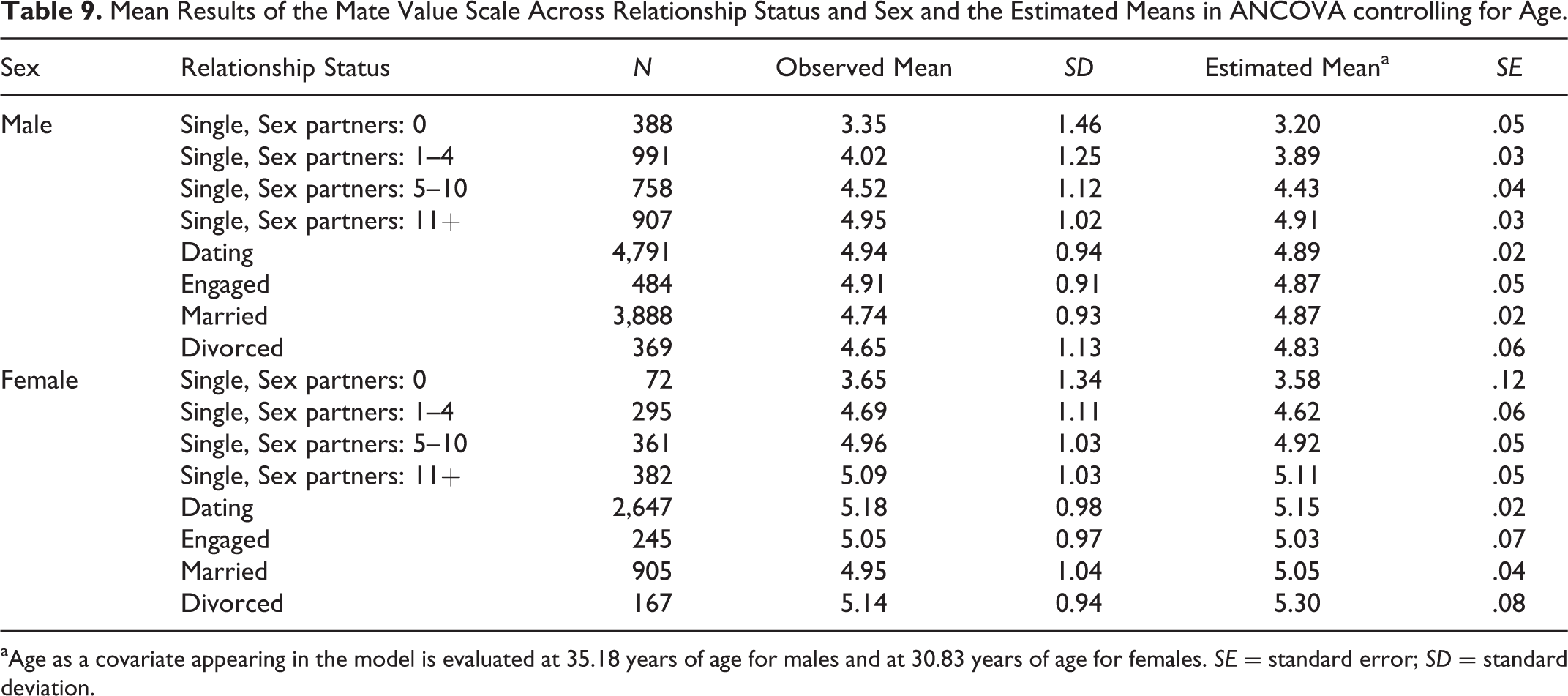
^aAge as a covariate appearing in the model is evaluated at 35.18 years of age for males and at 30.83 years of age for females. SE = standard error; SD = standard deviation.

Subsequently, we investigated whether relationship satisfaction affects self-perceived mate value. To avoid low frequency in some categories, we first pooled all participants who reported being in a relationship (i.e., dating, engaged, and married). The mate value of coupled individuals varying in their level of relationship satisfaction was then compared to single and divorced participants using a two-way ANCOVA with sex as another independent variable and age as a covariate. Single participants were again grouped according to the number of sexual partners they have had, the same way as in the previous analysis. Thus, what we below call “relationship satisfaction” was actually a complex variable, reflecting the complexity of the underlying phenomena.

The main effect of relationship satisfaction, F _satisfaction(7, 17631) = 169.516, p < .001, $η_{p}^{2}$ = .071; sex, F _sex(1, 17631) = 138.643, p < .001, $η_{p}^{2}$ = .008; age, (F _age(1, 17631) = 304.704, p < .001, $η_{p}^{2}$ = .017); and their interaction was significant, F _{satisfaction × sex}(7, 17631) = 9.237, p < .001, $η_{p}^{2}$ = .004. As predicted, relationship satisfaction was positively associated with self-perceived mate value. Again, as with relationship status, single participants with no or only a few previous sexual partners had the lowest self-perceived mate value, coupled participants had higher and differed according to how satisfied they were with their relationship, while divorcees (especially females) and singles with more than 10 previous partners had an MVS score comparable to that of people living in a good or happy relationship (for details, see Supplementary Material).

Finally, linear regression analyses were performed separately for the two sexes to assess the magnitude of a global effect of demographic variables on mate value. Since the R ² coefficients were of primary interest, only these are reported (for further details, see Supplementary Material). Taken together, level of education, SES, age, and relationship satisfaction variables (for the last one, the grouping of singles outlined previously was retained) predicted a significant but rather small part of the variance in self-perceived mate value, males: R ² = .196, F(15, 12767) = 208.843, p < .001; females: R ² = .108, F(15, 5179) = 43.006, p < .001. Moreover, of the independent variables, the strongest predictor of a low self-perceived mate value was being single with no previous sexual partners.

Discussion

Results of Study 2 again suggest that the MVS may be a reliable and valid measure of self-perceived mate value, although with important qualifications. To start with the positive findings, in the full CFA model, the latent mean of the MVS correlated positively with most minimum standard values for a potential partner, which indicates that people with a higher mate value do indeed have higher expectations about a potential partner in line with previous findings (Edlund & Sagarin, 2010; Regan, 1998; Wenzel & Emerson, 2009). In both sexes, the strongest correlation was found with passion and physical attractiveness. This is fully in line with findings reported in our earlier study (Csajbók & Berkics, 2017), where a self-assessed MVS score was predicted primarily by self-rated physical attractiveness.

It is very important, however, that relationships between demographic variables and mate value as measured by the MVS were in line with expectations regarding their direction only, but not their size. Although the differences between demographics were statistically significant, this was due to the large sample. The effect sizes were actually rather small, in most cases $η_{p}^{2}$ < .01. Only SES and relationship status had a larger (but still small) effect on self-perceived mate value, and even the effect of relationship status was mostly due to a remarkably low self-perceived mate value of single participants having had no (or only a few) previous sexual partners.

General Discussion

The research presented in this article started with the plausible and comfortable assumption shared by some of the previous literature that mate value can be measured in an easy way, simply asking people about it, because they have a by and large accurate sense of their own mate value, regardless of the complexities of the underlying processes and any awareness—or lack thereof—about them. However, in light of the results, one has to question this assumption.

From our two studies, we have two seemingly conflicting sets of findings. First, the MVS has good psychometric properties, performs well in CFA models, and is correlated to other measures in the expected way, especially strongly with self-esteem and almost as strongly with life satisfaction. On the other hand, whatever the scale measures it has only little to do with demographics, although evolutionary theory and a body of previous research implicate that “actual” mate value, measured in a more “objective” way, should vary considerably with age (especially for females) as well as with SES and education (especially for males). In our case, however, although most of these effects were statistically significant, the effect sizes were rather modest. Why, for example, do women in their early 40s have almost the same self-perceived mate value as women in their twenties? If the strongly underpinned and replicated evolutionary psychological theories are not supported by results obtained with a short measure of mate value, then the problem may lie with the measurement instrument.

When an instrument so simple and short is intended to measure a complex construct, some uncertainty regarding its conceptual clarity is possible to emerge. The apparent contradiction above might be resolved by considering “self-perceived” and “objective” mate value as two conceptually different constructs and considering the MVS as measuring self-perceived, but not objective mate value. This would explain why scores on the MVS hardly vary with demographics, although they are correlated quite strongly with self-esteem. In fact, the self-perception of mate value might be conceptually more akin to self-esteem than to objective mate value. This is not only suggested by our findings but can also be reasoned for with theoretical considerations.

Judgments are known to be subject to social comparisons (cf. Festinger, 1954) and also to goal-related comparisons. Self-esteem is just like that: It is not an indicator of one’s objective value in society but an indicator of, or feedback about, how well that person is doing relative to significant others or to relevant goals (cf. Leary & Baumeister, 2000). A biology teacher at the local school, for example, may have the same self-esteem as an eminent biologist at an Ivy League university. In fact, a local biology teacher whose students just won the county science competition may even have a somewhat higher self-esteem than a world-class biologist who just almost won the Nobel Prize. Certainly, both may be aware of the difference regarding their objective value in the science of biology, but this is hardly relevant to them as they are competing in different “leagues.”

Similarly, a 46-year-old woman may compare herself to other women of a similar age, and with regard to men in their late 40s or 50s as potential partners but not to women in their 20s or with the goal of acquiring a 30-year-old man as a long-term partner. Self-perceived mate value conceptualized this way, one should not expect any dramatic differences related to demographics, in this case to age.

This, of course, does not mean that self-perceived mate value should be considered useless as a psychological construct or as an operational variable. It only means that just as other subjective and relativistic self-perceptions, like self-esteem or life satisfaction, self-perceived mate value is also different from an objective mate value and may serve a different function. Although an objective mate value may put people into different leagues with regard to mating goals and strategies, competition, and social comparison, a self-perceived mate value may convey information about how well individuals are doing within their “league,” within the context of their goals, and levels of comparison. Indeed, besides being strongly correlated to self-esteem, self-perceived mate value as measured by the MVS also correlated—albeit not very strongly—with how high people would set their standards with regard to potential partners (cf. Edlund & Sagarin, 2010; Regan, 1998; Wenzel & Emerson, 2009). Of all demographic variables, relationship status combined with relationship satisfaction was one of the strongest predictors of MVS scores, while the strongest effect was that being single with no (or only a few) previous sexual partners that predicted a conspicuously reduced score. Despite the fact, as it was shown, self-perceived mate value is not objective, it can be a stronger predictor of mating-related behavior or preferences than mate value as perceived by others (see Arnocky, 2018). It may be, for instance, an important factor in determining whom one would approach as a potential partner, and who would be a target of jealousy and what intensity that jealousy would have.

Thus, the MVS indeed seems to be a reliable and valid instrument measuring self-perceived mate value, but with a strong emphasis on self-perceived. Further studies should be directed at a more objective mate value and the relationship between that and self-perceptions. Objective mate value may be operationalized in terms of transactions on the mating market. In economy, the price of goods is the amount of money paid when they are sold at a certain point in time under certain circumstances. Potential partners, however, are “goods” that are only supplied in one copy each and are exchanged rather than bought and sold, therefore, transactions involving them are rare and difficult to trace.

Measuring objective mate value, of course, would not be a process as easy and convenient as asking people to read and respond to four simple questions. The promise that a complex construct can be measured in a simple way was only partially fulfilled: We have an easy-to-measure construct, but it may not quite be the construct that was intended in the first place. At the same time, “objective mate value” can and should be conceptualized clearly, most probably in the way as values in economics go, that is, in terms of transactions on the mating “market”—but to its measurement, there is no royal road.

Supplemental Material

Supplemental Material, EP_mvs_supplement_20190111 - Self-Perceived Mate Value Is Poorly Predicted by Demographic Variables

Supplemental Material, EP_mvs_supplement_20190111 for Self-Perceived Mate Value Is Poorly Predicted by Demographic Variables by Zsófia Csajbók, Jan Havlíček, Zsolt Demetrovics, and Mihály Berkics in Evolutionary Psychology

Model	χ² (df)	CFI	TLI	RMSEA [90% CI]	Δχ² (df)	ΔCFI	ΔTLI	ΔRMSEA
Pooled	1,733.037 (529)	.940	.933	.045 [.043, .047]
Configural	2,218.085 (1,058)	.942	.935	.044 [.041, .147]
Metric (loadings)	2,293.237 (1,094)	.940	.935	.044 [.042, .047]	75.169 (36)	−.002	.000	.000
Scalar (intercepts)	2,514.515 (1,120)	.930	.926	.047 [.044, .049]	230.646 (26)	−.010	−.009	.003

Measures	1.	2.	3.	4.	5.	6.	7.	Std. Sex Diff.
1. MVS	—	.651***	.513***	−.391***	.183***	.164***	−.022	−.093
2. RSES	.631***	—	.671***	−.605***	.105*	.104*	−.121**	.159*
3. SWLS	.549***	.688***	—	−.593***	−.004	.063	−.181***	−.029
4. Loneliness	−.502***	−.647***	−.633***	—	−.064	.003	.300***	−.116
5. SOI behavior	.308***	.209***	.138**	−.200***	—	.653***	.355***	.060
6. SOI attitude	.123	.123	.040	−.016	.399***	—	.486***	.853***
7. SOI desire	−.103	−.140*	−.121*	.234***	.105	.440***	—	.926***

Sex	Age Groups (Years)	N	Mean	SD
Male	18–20	733	4.86	1.16
21–25	2,341	4.76	1.14
26–30	2,316	4.76	1.10
31–35	1,818	4.72	1.08
36–40	1,756	4.72	1.07
41–45	1,453	4.71	1.01
46–50	927	4.64	0.97
Older than 51	1,439	4.62	0.93
Female	18–20	432	5.03	1.06
21–25	1,523	5.11	0.95
26–30	1,171	5.13	1.07
31–35	669	5.16	1.00
36–40	478	5.00	1.04
41–45	401	4.97	1.06
46–50	258	4.75	1.11
Older than 51	263	4.78	1.04

Model	χ² (df)	CFI	TLI	RMSEA [90% CI]	Δχ² (df)	ΔCFI	ΔTLI	ΔRMSEA
Simple model (Mate Value Scale [MVS] only)—equivalence across sex and sexual orientation
Pooled	922.086 (2)	.982	.946	.148 [.140, .156]
Configural	962.848 (12)	.981	.944	.150 [.142, .158]
Metric (loadings)	1,002.393 (27)	.981	.974	.101 [.096, .107]	39.546(15)	.000	.030	−.049
Scalar (intercepts)	1,423.163 (42)	.973	.977	.097 [.092, .101]	420.770(15)	−.008	.003	−.004
Simple model (MVS only)—equivalence across age groups
Configural	882.806 (16)	.980	.941	.155 [.147, .164]
Metric (loadings)	944.837 (37)	.980	.973	.104 [.099, .110]	62.041(21)	.000	.032	−.041
Scalar (intercepts)	1,258.049 (58)	.973	.978	.096 [.091, .101]	313.202(21)	−.007	.005	−.008
Simple model (MVS only)—equivalence across education
Configural	805.963 (8)	.982	.946	.149 [.140, .158]
Metric (loadings)	845.871 (17)	.981	.973	.104 [.098, .110]	39.908(9)	−.001	.027	−.045
Scalar (intercepts)	983.523 (26)	.978	.980	.091 [.086, .095]	137.652(9)	−.003	.007	−.013
Simple model (MVS only)—equivalence across socioeconomic status
Configural	747.382 (8)	.982	.947	.143 [.135, .152]
Metric (loadings)	799.428 (17)	.981	.974	.101 [.095, .107]	52.045(9)	−.001	.027	−.042
Scalar (intercepts)	1,428.052 (26)	.966	.969	.110 [.105, .114]	628.625(9)	−.015	−.005	.009
Scalar (partial)^a	987.922 (25)	.977	.976	.097 [.092, .102]	188.494(6)	−.004	.002	−.004
Simple model (MVS only)—equivalence across relationship status
Configural	832.835 (12)	.980	.941	.152 [.143, .161]
Metric (loadings)	925.701 (27)	.979	.971	.106 [.100, .112]	92.866(15)	−.001	.030	−.046
Scalar (intercepts)	1,057.489 (42)	.976	.979	.090 [.086, .095]	131.788(15)	−.003	.008	−.016
Full model (MVS and minimum standards scales)—equivalence across sex
Pooled	10,431.191 (296)	.937	.925	.044 [.043, .044]
Configural	10,642.896 (592)	.934	.922	.043 [.043, .044]
Metric (loadings)	10,946.087 (611)	.933	.923	.043 [.043, .044]	306.605(19)	−.001	.001	.000
Scalar (intercepts)	12,863.778 (630)	.920	.911	.046 [.046, .047]	2,248.779(19)	−.013	−.012	.003
Scalar (partial)^b	12,068.345 (628)	.925	.917	.045 [.044, .046]	1,281.858(17)	−.008	−.006	.002

Latent factors	1.	2.	3.	4.	5.	6.	7.	8.	Std. Sex Diff.
1. MVS	—	.145	.064	.290	.331	.185	.162	.209	0.287***
2. MS warmth	.153	—	.737	.178	.289	.160	.389	.495	0.850***
3. MS stability	.022	.748	—	.106	.158	.191	.247	.313	0.248***
4. MS appearance	.347	.275	.161	—	.454	.442	.187	.292	−1.039***
5. MS passion	.342	.431	.304	.620	—	.314	.247	.526	0.052*
6. MS status	.132	.115	.181	.241	.247	—	.233	.362	0.780***
7. MS intellect	.193	.425	.281	.284	.304	.165	—	.420	0.593***
8. MS dominance	.183	.493	.418	.223	.469	.381	.483	—	1.200***

Sex	Sexual Orientation	N	Mean	SD
Male	Heterosexual	12,783	4.72	1.06
Heterosexual with some same-sex attraction	804	4.56	1.15
Bisexual	237	4.57	1.24
Homosexual with some opposite-sex attraction	99	4.49	1.23
Homosexual	445	4.76	1.14
Female	Heterosexual	5,195	5.06	1.03
Heterosexual with some same-sex attraction	1,128	5.12	1.00
Bisexual	326	4.94	1.24
Homosexual with some opposite-sex attraction	41	4.93	1.06
Homosexual	66	4.89	0.99

Sex	Level of Education	N	Mean	SD
Male	Primary	380	4.61	1.22
Vocational	778	4.53	0.96
High school	4,172	4.64	1.09
Higher education	7,453	4.80	1.04
Female	Primary	173	5.01	1.01
Vocational	116	4.99	1.00
High school	1,679	5.03	1.05
Higher education	3,227	5.08	1.02

Sex	SES	N	Mean of 4 Items	SD of 4 Items	Mean of 3 Items	SD of 3 Items
Male	Lower than average	632	3.97	1.23	3.86	1.29
Average	2,926	4.42	1.04	4.31	1.11
Somewhat better than average	5,614	4.73	1.02	4.59	1.10
Better than average	3,611	5.10	0.98	4.93	1.06
Female	Lower than average	203	4.44	1.23	4.34	1.30
Average	1,501	4.81	1.01	4.70	1.09
Somewhat better than average	2,216	5.12	0.98	5.01	1.05
Better than average	1,275	5.34	1.00	5.22	1.07

Sex	Relationship Status	N	Observed Mean	SD	Estimated Mean^a	SE
Male	Single, Sex partners: 0	388	3.35	1.46	3.20	.05
Single, Sex partners: 1–4	991	4.02	1.25	3.89	.03
Single, Sex partners: 5–10	758	4.52	1.12	4.43	.04
Single, Sex partners: 11+	907	4.95	1.02	4.91	.03
Dating	4,791	4.94	0.94	4.89	.02
Engaged	484	4.91	0.91	4.87	.05
Married	3,888	4.74	0.93	4.87	.02
Divorced	369	4.65	1.13	4.83	.06
Female	Single, Sex partners: 0	72	3.65	1.34	3.58	.12
Single, Sex partners: 1–4	295	4.69	1.11	4.62	.06
Single, Sex partners: 5–10	361	4.96	1.03	4.92	.05
Single, Sex partners: 11+	382	5.09	1.03	5.11	.05
Dating	2,647	5.18	0.98	5.15	.02
Engaged	245	5.05	0.97	5.03	.07
Married	905	4.95	1.04	5.05	.04
Divorced	167	5.14	0.94	5.30	.08

Footnotes

Acknowledgments

We thank all the respondents for their participation, Anna Pilátová, PhD for proofreading, and Zsolt Varga for data collection.

Declaration of Conflicting Interests

The author(s) declared no potential conflicts of interest with respect to the research, authorship, and/or publication of this article.

Funding

The author(s) disclosed receipt of the following financial support for the research, authorship, and/or publication of this article: The research was supported by the Hungarian National Research, Development and Innovation Office (grant numbers: K111938, KKP126835), and Czech Science Foundation Grant (18-15168S).

ORCID iD

Zsófia Csajbók

Mihály Berkics

Supplemental Material

Supplemental material for this article is available online.

Notes

References

Arnocky

(2018). Self-perceived mate value, facial attractiveness, and mate preferences: Do desirable men want it all? Evolutionary Psychology, 16.

Blake

K. R.

Bastian

O’Dean

S. M.

Denson

T. F.

(2017). High estradiol and low progesterone are associated with high assertiveness in women. Psychoneuroendocrinology, 75, 91–99.

Bőthe

Tóth-Király

Zsila

Á.

Griffiths

M. D.

Demetrovics

Orosz

(2018). The development of the problematic pornography consumption scale (PPCS). The Journal of Sex Research, 55, 395–406.

Brase

G. L.

Guy

E. C.

(2004). The demographics of mate value and self-esteem. Personality and Individual Differences, 36, 471–484.

Brindley

McDonald

M. M.

Welling

L. L.

Zeigler-Hill

(2018). An evolutionary perspective on intergroup dating bias. Comprehensive Results in Social Psychology, 3, 1–28.

Brown

(2006). Confirmatory factor analysis for applied research. New York, NY: Guilford Press.

Buss

D. M.

(1989). Sex differences in human mate preferences: Evolutionary hypotheses tested in 37 cultures. Behavioral and Brain Sciences, 12, 1–14.

Buss

D. M.

Schmitt

D. P.

(1993). Sexual strategies theory: An evolutionary perspective on human mating. Psychological Review, 100, 204–232.

Buss

D. M.

Shackelford

T. K.

(1997). From vigilance to violence: Mate retention tactics in married couples. Journal of Personality and Social Psychology, 72, 346–361.

10.

Campbell

Wilbur

C. J.

(2009). Are the traits we prefer in potential mates the traits they value in themselves? An analysis of sex differences in the self-concept. Self and Identity, 8, 418–446.

11.

Chen

F. F.

(2007). Sensitivity of goodness of fit indexes to lack of measurement invariance. Structural Equation Modeling, 14, 464–504.

12.

Csajbók

Berkics

(2017). Factor, factor, on the whole, who’s the best fitting of all? Factors of mate preferences in a large sample. Personality and Individual Differences, 114, 92–102.

13.

Diener

Emmons

R. A.

Larsen

R. J.

Griffin

(1985). The satisfaction with life scale. Journal of Personality Assessment, 49, 71–75.

14.

Edlund

J. E.

Sagarin

B. J.

(2010). Mate value and mate preferences: An investigation into decisions made with and without constraints. Personality and Individual Differences, 49, 835–839.

15.

Edlund

J. E.

Sagarin

B. J.

(2014). The mate value scale. Personality and Individual Differences, 64, 72–77.

16.

Erik

Bhogal

M. S.

(2016). Do the dark triad and self-perceived mate value predict intention to mate poach? Letters on Evolutionary Behavioral Science, 7, 1–4.

17.

Festinger

(1954). A theory of social comparison processes. Human Relations, 7, 117–140.

18.

Fisher

Cox

Bennett

Gavric

(2008). Components of self-perceived mate value. Journal of Social, Evolutionary, and Cultural Psychology, 2, 156.

19.

Fletcher

G. J.

Simpson

J. A.

Thomas

Giles

(1999). Ideals in intimate relationships. Journal of Personality and Social Psychology, 76, 72–89.

20.

Gillen

M. M.

Collisson

Murtagh

Browne

B. L.

McCutcheon

L. E.

(2016). Additional psychometric data for the mate value scale. Journal of Relationships Research, 7, 1–7.

21.

Goodwin

Marshall

Fülöp

Adonu

Spiewak

Neto

Hernandez Plaza

(2012). Mate value and self-esteem: Evidence from eight cultural groups. PLoS One, 7, e36106.

22.

Jonason

P. K.

Garcia

J. R.

Webster

G. D.

N. P.

Fisher

H. E.

(2015). Relationship dealbreakers: Traits people avoid in potential mates. Personality and Social Psychology Bulletin, 41, 1697–1711.

23.

Kasumovic

M. M.

Blake

Dixson

B. J.

Denson

T. F.

(2015). Why do people play violent video games? Demographic, status-related, and mating-related correlates in men and women. Personality and Individual Differences, 86, 204–211.

24.

Kenny

D. A.

Kaniskan

McCoach

D. B.

(2015). The performance of RMSEA in models with small degrees of freedom. Sociological Methods & Research, 44, 486–507.

25.

Kirkpatrick

L. A.

Waugh

C. E.

Valencia

Webster

G. D.

(2002). The functional domain specificity of self-esteem and the differential prediction of aggression. Journal of Personality and Social Psychology, 82, 756.

26.

Kirsner

B. R.

Figueredo

A. J.

Jacobs

W. J.

(2003). Self, friends, and lovers: Structural relations among Beck Depression Inventory scores and perceived mate values. Journal of Affective Disorders, 75, 131–148.

27.

Leary

M. R.

Baumeister

R. F.

(2000). The nature and function of self-esteem: Sociometer theory. In Advances in experimental social psychology (Vol. 32, pp. 1–62). Cambridge, MA: Academic Press.

28.

Lemay

E. P.

Jr & Wolf

N. R.

(2016). Projection of romantic and sexual desire in opposite-sex friendships: How wishful thinking creates a self-fulfilling prophecy. Personality and Social Psychology Bulletin, 42, 864–878.

29.

Luo

(2017). Assortative mating and couple similarity: Patterns, mechanisms, and consequences. Social and Personality Psychology Compass, 11, e12337.

30.

Mafra

A. L.

Lopes

F. A.

(2014). “Am I good enough for you?” Features related to self-perception and self-esteem of Brazilians from different socioeconomic status. Psychology, 5, 653–663.

31.

March

Wagstaff

D. L.

(2017). Sending nudes: Sex, self-rated mate value, and trait Machiavellianism predict sending unsolicited explicit images. Frontiers in Psychology, 8, 2210.

32.

Martos

Sallay

Désfalvi

Szabó

Ittzés

(2014). Az Élettel való Elégedettség Skála magyar változatának (SWLS-H) pszichometriai jellemzői [Psychometric characteristics of the Hungarian version of the Satisfaction with Life Scale (SWLS-H)]. Mentálhigiéné és Pszichoszomatika, 15, 289–303.

33.

McDonald

M. M.

Coleman

Brindley

(2019). Calibrating fear of rape: Threat likelihood and victimization costs. Personality and Individual Differences, 139, 326–330.

34.

Meskó

Láng

Kocsor

Rózsa

(2012). Measuring sexual commitment. Hungarian version of the sociosexual orientation inventory revised (SOI-R). Magyar Pszichologiai Szemle, 67, 733–755.

35.

Pass

J. A.

Lindenberg

S. M.

Park

J. H.

(2010). All you need is love: Is the sociometer especially sensitive to one’s mating capacity? European Journal of Social Psychology, 40, 221–234.

36.

Penke

Asendorpf

J. B.

(2008). Beyond global sociosexual orientations: A more differentiated look at sociosexuality and its effects on courtship and romantic relationships. Journal of Personality and Social Psychology, 95, 1113–1135.

37.

Penke

Denissen

J. J.

(2008). Sex differences and lifestyle-dependent shifts in the attunement of self-esteem to self-perceived mate value: Hints to an adaptive mechanism? Journal of Research in Personality, 42, 1123–1129.

38.

Peplau

L. A.

Cutrona

C. E.

(1980). The revised UCLA Loneliness Scale: Concurrent and discriminant validity evidence. Journal of Personality and Social Psychology, 39, 472–480.

39.

Regan

P. C.

(1998). What if you can’t get what you want? Willingness to compromise ideal mate selection standards as a function of sex, mate value, and relationship context. Personality and Social Psychology Bulletin, 24, 1294–1303.

40.

Roberts

B. W.

Donahue

E. M.

(1994). One personality, multiple selves: Integrating personality and social roles. Journal of Personality, 62, 199–218.

41.

Rosenberg

(1965). Rosenberg self-esteem scale (RSE). Acceptance and Commitment Therapy: Measures Package, 61, 52.

42.

Sallay

Martos

Földvári

Szabó

Ittzés

(2014). Hungarian version of the Rosenberg Self-esteem Scale (RSES-H): An alternative translation, structural invariance, and validity. Mentálhigiéné és Pszichoszomatika, 15, 259–275.

43.

Shackelford

T. K.

(2001). Self-esteem in marriage. Personality and Individual Differences, 30, 371–390.

44.

Singh

(2002). Female mate value at a glance: Relationship of waist-to-hip ratio to health, fecundity and attractiveness. Neuroendocrinology Letters, 23, 81–91.

45.

Symons

(1985). Darwinism and contemporary marriage. In Davis

Grossbard-Shechtman

(Eds.), Contemporary Marriage (pp. 133–155). New York, NY: Russell Sage Foundation.

46.

Trivers

(1972). Parental investment and sexual selection (Vol. 136). Cambridge, MA: Biological Laboratories, Harvard University.

47.

Urbán

Szigeti

Kökönyei

Demetrovics

(2014). Global self-esteem and method effects: Competing factor structures, longitudinal invariance and response styles in adolescents. Behavior Research Methods, 46, 488.

48.

Wenzel

Emerson

(2009). Mate selection in socially anxious and nonanxious individuals. Journal of Social and Clinical Psychology, 28, 341–363.

49.

Zhang

Liu

Ruan

L. J.

(2015). Heterosexual rejection and mate choice: A sociometer perspective. Frontiers in Psychology, 6, 1846.

Supplementary Material

Please find the following supplemental material available below.

For Open Access articles published under a Creative Commons License, all supplemental material carries the same license as the article it is associated with.

For non-Open Access articles published, all supplemental material carries a non-exclusive license, and permission requests for re-use of supplemental material or any part of supplemental material shall be sent directly to the copyright owner as specified in the copyright notice associated with the article.

0.00 MB

0.71 MB