
Abstract
This study provides independent empirical evidence that bears upon the truth or falsity of recently formulated hypotheses regarding reciprocal relationships between levels of religiosity and societal dysfunction. Gregory S. Paul's findings, published in the Journal of Religion and Society (2005), Free Inquiry (2008), and Evolutionary Psychology (2009), have demonstrated that high degrees of theism are associated with high degrees of societal dysfunction among the prosperous democracies. Whereas his research employs numerous scatter diagrams and bivariate correlations involving measures of religiosity and societal dysfunction pertaining to 17 nation states, the current study's units of analysis are the 50 states and the District of Columbia. Additionally, the utilization of multiple regression analysis allows the detection of the effects of other potentially relevant explanatory variables, such as educational attainment, income level, and race. The findings are only minimally supportive of Paul's hypotheses regarding the contributions of high religiosity to societal dysfunction and to the effects of societal dysfunction upon religiosity. Simultaneously, the results of correlational and regression analyses attest to the more substantial explanatory power of the social inequality variables of education, income, and race. Accordingly, it is argued that “American Exceptionalism,” when understood as referring to a society manifesting the coexistence of high levels of theism and high levels of societal dysfunction, is best explained by the United States' high degree of social inequality, compared with other modern industrialized democracies.
Keywords
Introduction
The findings of recent sociological studies by Paul (2005, 2008, 2009) suggest a pressing need for a revised definition of “American Exceptionalism” as that term has been commonly understood in the United States. Paul's empirically-based explication of the term would have been unimaginable by Alexis de Tocqueville whose Democracy in America (1835) is often cited as the source for the canonizing metaphor describing the U.S. as the “shining city on the hill.”
Whereas Tocqueville applauded the fledgling democracy that was the young U.S. as the exemplar of human liberty and equality, Paul's empirical inquiries have uncovered the country's exceptionalness in a much less flattering sense: It is unique among 17 prosperous Western industrialized democracies as being the most dysfunctional in terms of a wide variety of measures of societal health, including having the highest rates of homicide; incarceration; infant mortality; and teen pregnancies, abortions and births. Its population also evidences poorer physical health and shorter life expectancies than might be predicted on the basis of the country's enormous comparative wealth advantages as measured by its Gross Domestic Product.
Utilizing scatter diagrams and bivariate correlational analyses, Paul has demonstrated that the most dysfunctional of the modern democracies is also the most theistic in terms of a variety of indicators of religious beliefs and practices, such as belief in God or universal spirit, importance of religion in everyday life, belief in the inerrancy of the Bible, frequency of attendance at religious services, frequency of prayer, and belief in creationism, with a corresponding rejection of the Darwinian “theory” of evolution.
Paul's research findings have justified his formulation of several hypotheses regarding the relationships between religiosity and societal dysfunction, in light of the increases in modernization and secularization that have been experienced by the prosperous democracies. For details, the reader is referred to his “Cross-National Correlations of Quantifiable Societal Health with Popular Religiosity and Secularism in the Prosperous Democracies” (2005); “The Big Religion Questions Finally Solved” (2008); and “The Chronic Dependence of Popular Religiosity upon Dysfunctional Psychosociological Conditions” (2009).
Concisely stated, Paul's two basic hypotheses are:
High levels of theism contribute to high levels of societal dysfunction.
High levels of societal dysfunction contribute to the persistence of theistic beliefs and practices.
If true, both hypotheses help explain “American Exceptionalism,” i.e., extreme levels of both theism and societal dysfunction when compared with the other prosperous democracies. Also, the first would lead to the prediction that decreases in religiosity in the U.S. will affect increases in societal health, while the second suggests that reductions in levels of societal dysfunction will lead to decreased religiosity.
It is anticipated that the findings of the current empirical inquiry will provide additional independent evidence related to the truth or falsity of Paul's hypotheses, but before describing the purposes, methods, and procedures of the current research, it is important to make mention of a number of criticisms by social and behavioral scientists of the reliability and validity of Paul's findings based upon the methodology employed in his research, especially his 2005 Journal of Religion and Society article.
Moreno-Riaño, Smith, and Mach (2006) precede their specific criticisms of Paul's work with the following:
Paul's efforts and “first look” should be applauded since they bring to the attention of religious studies scholars and social scientists a very important and timely subject of study. At the same time, the scholarly community, in the spirit of constructive and critical scientific inquiry, needs to assess the methodological assumptions which frame Paul's investigation (p. 1).
Their own review of Paul's methodology prompts them to assert that:
It is the opinion of the authors that once all of the methodological issues are considered, Paul's findings and conclusions are rendered ineffectual (p. 2).
Their thorough and detailed critique of Paul's 2005 study includes discussion of errors related to “methodological individualism,” “conceptual ambiguity,” “comparative analysis and operationalizations,” and “real versus artifactual differences.” They conclude their examination by asserting that “What one can state with certainty is that one cannot in any way be certain as to the effects of religiosity and secularism upon prosperous democracies at least as based upon the methods and data of Paul's study” (p. 9).
In his “The Complexities of Comparative Research” (2008), Stark accuses Paul of committing the egregious error of not considering or controlling for the ecological fallacy as well as cherry-picking of cases and variables, and not considering the lack of compatibility among cases. It is telling that Stark asserts that:
Perhaps the best way to reveal the complexities of using collective units of analysis is to examine a recent study [Paul's] that received a great deal of favorable praise in the international news media and that continues to enjoy considerable celebrity on the Internet, despite being a worthless concoction of nonsense (p. 9) (italics added).
It is anticipated that the methods utilized in the current study will prove to be somewhat more cautious and effective in dealing with the pitfalls of comparative research involving ecological units of analysis.
Materials and Methods
This study is designed as a modified replication of Paul's research, the primary differences being the units of analysis and the statistical techniques utilized. Whereas his study is based upon a large number of scatter diagrams and bivariate correlational analyses of religiosity and societal health indicators pertaining to 17 countries, thereby representing a cross-national perspective, the current research utilizes multivariate regression analyses applied to the 50 U.S. states and the District of Columbia. Statistically speaking, the advantages of the current research are two-fold: multivariate regression analyses allow for the examination of the influence of other potentially relevant explanatory variables in addition to religiosity as they might affect levels of societal dysfunction; and the sample size (n = 51) of the 50 states and the District of Columbia is three times larger than Paul's, allowing greater confidence in the statistical significance of the findings.
Indicators of societal dysfunction
Thirteen indicators of societal dysfunction are used in the current research, and they are subsumed under the following four categories of dysfunctionality: Crime and Punishment (“Violent Crime Rate,” “Murder Rate,” and “Incarceration Rate”); Teen Reproductive Behavior (“Pregnancy Rate,” “Abortion Rate,” and “Birth Rate,”): Health and Morbidity (“Adult Obesity Rate,” “Adult Smoking Rate,” “Alcohol Consumption,” and “Overall Health”); and Mortality (“Infant Mortality Rate,” “Life Expectancy,” and “Suicide Rate”). The relevant data are derived from a variety of sources, including the U.S. Census Bureau, the Centers for Disease Control, the Bureau of Justice Statistics, the Guttmacher Institute, and a number of other reliable online and print sources, all of which are included below among the references cited.
Admittedly, this is only a partial list of the wide variety of indicators of societal health that have been identified by nations and international organizations such as the World Health Organization (WHO) and the Organization for Economic Cooperation and Development (OECD). Among the indicators not dealt with in this study but included in Paul's (2005, 2009) research, for example, are sexually transmitted disease rates, such as rates for gonorrhea and syphilis; marriage and divorce; corruption indices; life satisfaction; employment levels; resource exploitation base; acceptance of “human descent from animals”; among others. It is expected and hoped that the methods utilized in the current study will stimulate research involving other measures of societal health.
Indicators of high religiosity
The selection of an appropriate measure or measures of religiosity is rendered particularly challenging because of the numerous possible indicators that are available for secondary analysis and that have been utilized in other studies, both within the U.S. and in cross-national research, such as denominational affiliation (e.g., Protestant, Catholic, Jewish, Muslim, Hindu), belief in God or universal spirit, interpretation of scripture (e.g., Biblical literalism), importance of religion in everyday life, frequency of attendance at religious services, frequency of prayer, belief in life after death, and the existence of heaven and hell, among others.
Norris and Inglehart (2004), for example, in their substantial contribution to comparative cross-national research include consideration of “Type of Religious Culture” (Eastern, Hindu, Jewish, Muslim, Orthodox, Other, Protestant, Roman Catholic) (p. 45); “Religious Participation” (frequency of attendance at religious services and frequency of prayer); “Religious Values” (importance of God in one's life, importance of religion in one's life); “Religious Beliefs” (belief in heaven, hell, life after death, and people having a soul) (p. 41); and “Religious Markets” (religious pluralism, Religious Freedom Index, state regulation of religion, Freedom House religious freedom scale) (p. 99).
Reese (2009) utilizes frequency of prayer as the measure of religiosity for his research, while Jensen (2006) develops composite measures based on several beliefs and practices including, for example, “Intensity,” “Malevolent,” “Benevolent,” “Ritual”; and “Secular,” “God-Only,” and “Dualist.”
In American Piety in the 21 st Century: New Insights to the Depth and Complexity of Religion in the U.S. (2006), Stark and his colleagues at The Baylor Institute for Studies of Religion, presenting “Selected Findings from The Baylor Religion Survey,” involving a nationally representative, probability sample which was conducted in 2005, describes the congregational and denominational affiliations of the 1,721 respondents as self-identifying with the following traditions: Catholic (21.2%), Black Protestant (5%). Evangelical Protestant (33.6%), Mainline Protestant (22.1%), Jewish (2.5%), Other (4.9%), and Unaffiliated (10.8%) (p. 8). Acknowledging the declining importance of denominational affiliation at a time when many Americans are abandoning the traditional mainline denominations in favor of increasingly numerous non-denominational congregations, as well as the great variety of religious beliefs and practices exhibited by both the affiliated and unaffiliated, Stark argues that religiosity is more appropriately measured by beliefs and practices, such as “Belief about God,” “Belief about Jesus,” “Belief about Bible,” “Pray,” “Read Scripture,” and “Attend Religious Services” (p. 14).
Stark also describes the respondents of the Baylor survey in terms of their identification with “selected religious labels,” including “Bible-Believing” (47.2%), “Born Again” (28.5%), “Mainline Christian” (26.1%), “Theologically Conservative” (17.6%), “Evangelical” (14.9%), “Theologically Liberal” (13.8%), “Moral Majority” (10.3%), among several others with fewer than 10% self-identifying, including “Religious Right” (8.3%), and “Fundamentalist” (7.7%) (p. 16).
Based upon respondents' answers to some 29 survey questions about God's character and behavior, Stark and his colleagues performed a factor analysis that revealed “two clear and distinct dimensions of belief in God:”
God's level of engagement – the extent to which individuals believe that God is directly involved in worldly and personal affairs. [and]
God's level of anger – the extent to which individuals believe that God is angered by human sins and tends towards punishing, severe, and wrathful characteristics. (p. 26)
These two dimensions are utilized to develop the “Categories of America's Four Gods.” (pp. 26–27). Individuals who are high on the dimension of God is Angry and high on the dimension that God is Engaged worship the “Type A: Authoritarian God;” those who are low on God is Angry and low on God is Engaged worship the “Type D: Distant God;” and those who high on God is Angry but low on God is Engaged fall into the “Type C: Critical God” category, while their opposites, low on God is Angry, but high on God is Engaged” believe in the “Type B: Benevolent God” (pp. 26–67). The percentages of the survey respondents falling into these categories are 31.4% in Type A, 23.0% in Type B, 16% in Type C, and 24.4% in Type D. Excluded from the above categories were the 5.2% self-identified atheists in the sample.
Stark subsequently examines the relationships between the four God categories and a variety of respondent demographic characteristics as well as the several religious beliefs and practices already discussed (pp. 28–31).
Altogether, Stark's multivariate and multi-dimensional investigation into the interrelationships among denominational affiliation and religious beliefs and practices represents an important contribution to a better understanding into the “Depth and Complexity of Religion in the U.S.” as the research report's subtitle promises, and it has influenced the methodology employed in the current study to develop a unique composite measure of high religiosity.
Composite measure of high religiosity
The composite measure developed for this study is based upon responses to six questions asked in the 2007 Pew Forum on Religion and Public Life Religious Landscape Survey's national probability sample of more than 35,000 respondents (2009). Among the several dimensions of religiosity examined in the Pew research were denominational identification, and beliefs and practices. The composite measure of high religiosity includes the percentage of U.S. states' respondents selecting the first response alternative within each of the following categories:
Denominational affiliation
Evangelical Protestant Tradition (26% of the Pew sample)
Mainline Protestant Tradition (18%)
Historically Black Protestant Tradition (7%)
Catholic Tradition (24%)
Unaffiliated (16%)
All Other (9%, with none of the other 10 traditions or faiths having more than 2%, including Muslims and Jews)
Belief regarding the existence of God or universal spirit
Absolutely certain that God exists (71%)
Fairly certain (17%)
Not too certain/not at all certain/unsure how certain (4%)
Does not believe in God (5%)
Don't know/refused to answer/other (3%)
Belief regarding interpretation of Scripture [Bible or Holy Book]
Word of God, literally true, word for word (33%)
Word of God, but not literally true word for word/unsure if literally true (30%)
Book written by man, not the word of God (28%)
Don't know/refused/other (9%)
Belief [or value] regarding importance of religion in one's life
Very important (56%)
Somewhat important (26%)
Not too important/not at all important (16%)
Don't know/refused (1%)
Frequency of attendance at religious services
At least once a week (39%)
Once or twice monthly/few times a year (33%)
Seldom or never (27%)
Don't know/refused (1%)
Frequency of prayer
At least once a day (58%)
Once a week/a few times a week (17%)
A few times a month (6%)
Seldom or never (18%)
Don't know/refused (2%)
The results of a principal components analysis of the percentage of state respondents selecting the first alternative to the above questions provides the basis for the operational definition of the composite measure of high religiosity. The principal components analysis results are shown in Table 1. The variable names or labels and definitions for all variables utilized in this study are displayed in Appendix A.
Summary results of principal components analysis for six religiosity variables: EVANPROT “evangelical protestant;” ABSCERT “absolutely certain that God exists;” WORDGOD “Bible is word of God, literally true, word for word;” VERYIMPO “religion is very important in everyday life;” SERVWEEK “attend religious services at least once a week;” and PRAYDAY “pray at least once a day.” n = 51 (U.S. States and D.C.)

Each of the correlation coefficients in Table 1 is significant at p < .0001, and the r values indicate strong positive associations between the selected variables of high religiosity. In addition, the results of the principal components analysis demonstrate the existence of one principal component that may be reasonably interpreted as indicative of a single dimension of high religiosity. This composite measure of high religiosity, HIGHREL, is operationally defined as the combination (sum) of the z scores for EVANPROT, ABSCERT, WORDGOD, VERYIMPO, SERVWEEK, and PRAYDAY. The combined z scores for the 50 U.S. States and the District of Columbia appear in Table 2, and are displayed in decreasing order of z values for HIGHREL.
High religiosity for the U.S. States and the District of Columbia in 2007 (Pew 2009), based on the composite index HIGHREL

The operational definition of high religiosity as a composite measure of denominational affiliation and religious beliefs and practices corresponds most closely to, and receives validation from, Stark's “Type A – Authoritarian God,” namely a God who is both “Angry” and “Engaged” in the affairs of this world. Respondents participating in The Baylor University Religion Survey of 2005, who were characterized as believing in an Authoritarian God, were more likely to identify with the Protestant Evangelical tradition, believe that the Bible is the actual word of God, attend church at least once a week, and pray several times a day (2006, p. 30).
Control variables
Since I am interested in examining the relationships between high levels of religiosity and the several indicators of societal dysfunction previously identified, I must demonstrate that whatever relationships we might uncover are not spurious and this objective may be achieved, at least approximately, by controlling for the effects of other potentially confounding variables. The selection of these variables is guided by the findings of previous research involving relationships between variations in socioeconomic status, including the concept of relative deprivation, and religious beliefs and practices, as evidenced in studies such as those by Schieman (2010), Davidson (1977), Mirowski (1999), Mirowski and Ross (2003), Pyle (2006), Stark (1972), Van Roy, Bean, and Wood (1973), and McCloud (2007). Of particular relevance to the current study is the theoretical framework developed by Norris and Inglehart in their comparative, cross-national study, Sacred and Secular (2004).
Attempting to reconcile the alternative explanations for religiosity and religious behavior offered by proponents and opponents of the secularization hypothesis, Norris and Inglehart seek a middle-ground or synthesis by invoking the concept of societal and personal insecurity (pp. 3–32). In their words:
There is no question that the traditional secularization thesis needs updating. It is obvious that religion has not disappeared from the world, nor does it seem likely to do so. Nevertheless, the concept of secularization captures an important part of what is going on. This book Sacred and Secular develops a revised version of secularization theory that emphasizes the extent to which people have a sense of existential security – that is, the feeling that survival is secure enough that it can be taken for granted. We build on key elements of traditional sociological accounts while revising others. We believe that the importance of religiosity persists most strongly among vulnerable populations, especially those living in poorer nations, facing personal survival-threatening risks. We argue that feelings of vulnerability to physical, societal, and personal risks are a key factor driving religiosity and we demonstrate that the process of secularization – a systematic erosion of religious practices, values, and beliefs – has occurred most clearly among the most prosperous social sectors living in affluent and secure post-industrial nations (pp. 4–5).
Norris and Inglehart go on to amass a substantial body of cross-national, comparative data to support their case. If we accept the soundness of their reasoning and empirical findings, we might hypothesize that variations in existential security among certain identifiable population subgroups or segments within post-industrial nations ought similarly to relate to varying degrees of religiosity. Indeed, this hypothesis has been at least partially confirmed by Reese in his “Is personal insecurity a cause of cross-national differences in the intensity of religious belief?” (2009) as well as by Schieman in “Socioeconomic status and beliefs about God's influence in everyday life” (2010). Rees demonstrates the importance of income inequality to the explanation of variations in degrees of personal religiosity, while Schieman zeros in on “the relevance of SES – as indexed by education and income.”
In fact, Schieman (2010) provides perhaps the most comprehensive contemporary overview of the research pertaining to the relationships between the key dimensions of social stratification, namely, education and income, and religiosity. The following passage is worth quoting in its entirety:
First and foremost, these represent the core dimensions of social stratification that have implications for an array of personal, social, and health advantages (Mirowsky and Ross, 2003). Prior research has drawn attention to education's role in understanding variations in the nature and functions of religious precepts and practices. Pollner (1989), for example, hypothesized that education modifies the psychological effects of religiosity because of its association with cognitive abilities and an enhanced capacity to comprehend “complex symbolic codes.” Pollner's thesis implies that people with less education “may profit especially from the sense of order and meaning generated in and through divine interaction”…likewise, theoretical views about deprivation–compensation are potentially relevant (Wilson, 1982). Individuals in disadvantaged socioeconomic conditions are purportedly more likely to construct a bond with the divine to compensate for their plight and acquire otherwise–unattainable rewards (Glock and Stark 1965; Stark 1972). This thesis posits that reliance upon an omnipotent deity who is perceived as satisfying desires may offset the deleterious psychological effects of immutable adversities in everyday life. Consistent with this view, substantial evidence confirms that low SES individuals are more likely to seek God's will through prayer (Albrecht and Heaton 1984), and tend to report higher levels of divine interaction (Pollner 1989), feeling connected with God (Krause 2002), religious meaning and coping (Krause 2003, 1995), God-mediated control (Krause 2005, 2007), and the sense of divine control (Schieman et.al. 2006). Moreover, low SES groups tend to derive greater psychological benefits from religiosity (Ellison 1991; Krause 1995; Pollner 1989). (p. 4)
In addition to the core SES variables of education and income, informed understanding of the contemporary realities of social inequality in the U.S. must of necessity include a consideration of race, a signifier of social and personal identity that, like education and income, has important implications for the life chances of members of racial minorities, including African Americans, Hispanic Americans, and Native Americans. African Americans have a long history of being victims of prejudice and discrimination from the days of the slave-based Southern agricultural economy, through the post-Reconstruction period of oppressive Jim Crow laws to the more modern forms of institutional racism, as evidenced by differential educational and employment opportunities as well as regarding housing and access to health care (Better, 2007; Davis, 2006; Feagin, 2007; Marger, 2008; Pettus, 2004; West, 2001; Wilson 1990, 1997, 2007, 2010).
Differences in educational attainment, level of income, and race are fundamental to understanding the contemporary realities of social inequality in the United States, and, as sources of social and personal insecurity, must be considered as potentially important control variables in any inquiry into the relationships of religiosity and societal dysfunction. Accordingly, they are included in each of the several analyses in the following presentation of the findings.
In both Parts I and II of the following section, the Ordinary Least Squares (OLS) program developed by Bill Miller and available online at www.OpenStat.org was utilized for each procedure. Implementation of this statistical technique produces results that show the separate effects of each of the independent variables on the dependent variable.
Results
Part I
In this section, we present the results of 13 multivariate OLS regression analyses that bear upon the truth or falsity of Paul's first hypothesis, namely:
High levels of theism contribute to high levels of societal dysfunction.
Correlation matrix for high religiosity (HIGHREL) and the OLS control variables educational attainment of bachelor's degree or higher (BACHPLUS), median household income (INCOME) and percent of African Americans (RACE)

Note:
p < .001; n = 51 (U.S. States and D.C.)
These data reveal statistically significant and large negative relationships between both BACHPLU S and INCOME with HIGHREL and a moderate positive relationship between RACE and HIGHREL. A number of the other correlations between our control variables are also moderate to large, indicating the need for diligence in the detection of possible problems with mulitcollinearity in our OLS regression analyses. Examination of the VIF (Variation Inflation Factor) values associated with all of the regression analyses shows no evidence of multicollinearity.
Crime and punishment
According to cross-national statistics, the U.S. has the highest rates of both crime and punishment among the “First-World” countries. In 2008, the U.S. murder rate (number of intentional homicides per 100,000 population) was 5.40, compared with 2.26 for Switzerland, 2.03 for United Kingdom, 1.87 for Israel, 1.83 for Canada, 1.59 France, .89 Sweden, and .44 for Japan (U.S. Bureau of Justice Statistics, Federal Bureau of Investigation, 2006).
In 2007, U.S. prisons held 2,293,157 inmates, which represented an incarceration rate of 756 prisoners per 100,000 population. By comparison, incarceration rates for other Western industrialized nations were: Canada at 116, Israel 326, Sweden 74, England and Wales 153, France 96, and Germany 89 (International Centre for Prison Studies 2008).
Official government sources show wide variation in murder rates and violent crime rates within the U.S., but the largest variation among states is in regard to incarceration rates, ranging from a per 100,000 population high of 1,138 in Louisiana to 273 in Maine (U.S. Bureau of Justice Statistics 2005). Basic descriptive statistics of central tendency and variability for each of the crime and punishment measures, as well as for all other variables utilized in this study are displayed in Appendix B. State-by-state values on all indicators are available by consulting the original data sources cited in the References.
Table 4 displays the OLS regression results for violent crime rates (VICRATES) regressed on the measure of high religiosity (HIGHREL) and the control variables of educational attainment of bachelor's degree or higher (BACHPLUS), median household income (INCOME) and the percentages of state populations who are African American (RACE).
OLS regression of violent crime rates (VICRATE) on high religiosity (HIGHREL), educational attainment of bachelor's or higher (BACHPLUS), median household income (INCOME), and percent of African Americans (RACE)

Note:
p < .001; n = 51 (U.S. States and D.C.)
Examination of the correlation coefficients of column 1 reveals a non-significant positive correlation between HIGHREL and VICRATE (.195), and the unstandardized B and its relatively large associated standard error (s.e.b.) yield a significance level value (p) (based on the t-test) that is non-significant. Accordingly, the results provide no evidence of high religiosity being a contributor to violent crime rates in the U.S, when controlling for BACHPLUS, INCOME and RACE. The correlational relationships are thereby revealed to be spurious, at least to some degree. The same lack of low predictive or explanatory value is observable regarding the control variables of BACHPLUS and INCOME. In sharp contrast to these findings, the percent of state populations who are African Americans shows a large positive r of .694, and the OLS regression statistics reveal it to be the best predictor of violent crime rates in the analysis, with a t-test statistic result of p < .001. The Beta value of .792 is also relatively high, and the proportion of variation in violent crime rates accounted for or explained by the analysis is a statistically significant R 2 value of .5046 (Adjusted R 2 = .4615). The ANOVA results for the regression analysis (not shown) yielded an F value of 11.715, which is significant at p < .0001. VIF (Variance Inflation Factor) values for the OLS analysis show no evidence of multicollinearity. It is RACE, therefore, and not HIGHREL that is most highly related to VICRATE in the U.S. The higher the percentage of African Americans within states, the higher the violent crime rate.
OLS regression of murder rates (MURRATE) on HIGHREL, BACHPLUS, INCOME, and RACE

Note:
p < .001; n = 51 (U.S. States and D.C.)
The r values indicate a moderate positive and significant relationship between MURRATE and HIGHREL, a low positive and non-significant relationship between MURRATE and BACHPLUS, and a very low negative and non-significant relationship between MURRATE and INCOME. Similar to the findings regarding violent crime rates, however, the control variable of RACE is the best predictor of the dependent variable, in this case, MURRATE. The higher the percentage of African Americans within states, the higher the murder rate.
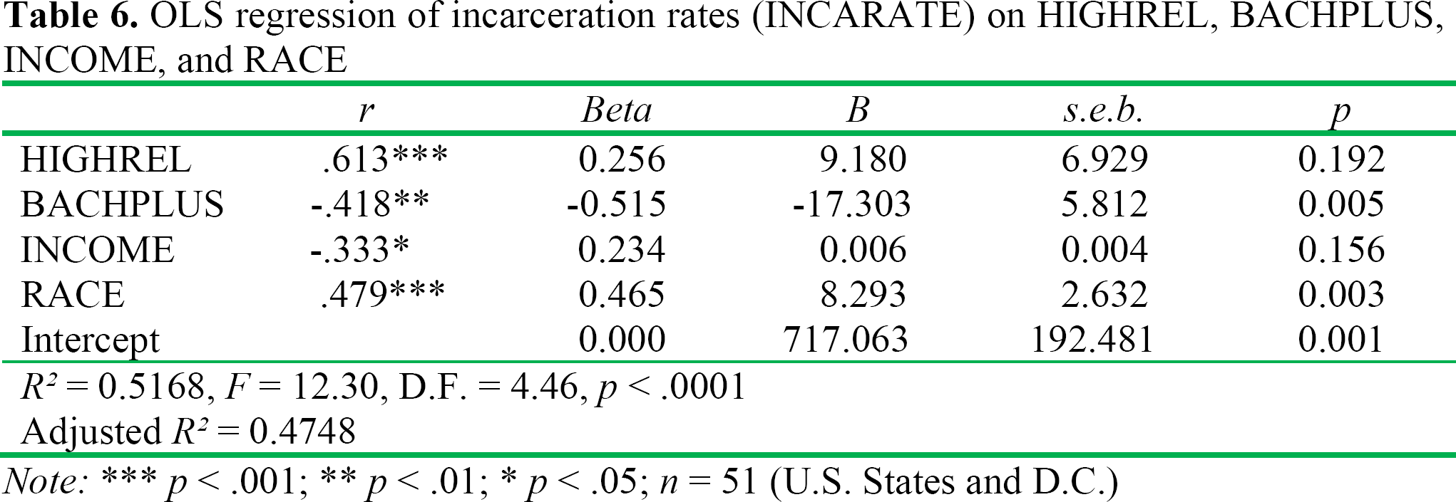
OLS regression of incarceration rates (INCARATE) on HIGHREL, BACHPLUS, INCOME, and RACE
Note:
p < .001
p < .01
p < .05; n = 51 (U.S. States and D.C.)
The .613 correlation between HIGHREL and INCARATE in column 1 is indicative of a high positive relationship. The BACHPLUS and INCOME r values of −.418 and −.333, respectively, demonstrate moderate negative relationships. The .479 value at the bottom of that column shows a moderate positive relationship between RACE and INCARATE. Comparing the Beta, B, s.e.b. and p regression analysis values with their counterparts in the two immediately preceding tables reveals HIGHREL to be a numerically better predictor of INCARATE than of VICRATE and MURRATE. In this analysis, however, BACHPLUS and RACE demonstrate the greatest predictive power, with high levels of educational attainment associated with low incarceration rates, and high percentages of African Americans associated with high incarceration rates. The higher the level of religiosity, the higher the incarceration rate. The higher the level of educational attainment, the lower the incarceration rate. The higher the percentage of African Americans, the higher the incarceration rate.
Teen reproductive behavior
The teen years (ages 15–19 years in archival datasets used in current analyses) for both males and females in the U.S. are of special importance in representing the time when most are or should be progressing successfully through the grades of secondary school and, ideally, going on to pursue post-secondary work at a two-year community or technical college or at a public or private four-year college or university offering a bachelor's degree that still serves as the basic, and now usually only minimal, credential necessary for entry into most professional occupations. Females face a particular challenge during these typically life-defining years, because of the possibility that they may become pregnant.
International data show the United States scoring highest on various indicators of teen reproductive behavior in comparison with other industrial democracies. In 1998, the most recent year for which cross-national statistics are available, the U.S. recorded 1,671.63 pregnancies to women aged below 20 years per one million population. The rate for Canada, by contrast, was 607.22, for Germany 351.81, France 296.51, Sweden 178.29, and Japan 137.35. The teen birth rates, number of births for every 1,000 girls ages 15–19, among these same countries were: United States 64, Canada 27, Germany 13, France 9, Sweden 13, and Japan 4 (UNICEF, 1998).
In Table 7 are presented the OLS regression results for teen (ages 15–19 years) pregnancy rates (PREGRATE) regressed on high religiosity (HIGHREL) along with the control variables of educational attainment of a bachelor's degree or higher (BACHPLUS), median family income (INCOME) and percentage of African Americans (RACE).
OLS regression of pregnancy rates (PREGRATE) on HIGHREL, BACHPLUS, INCOME, and RACE

Note:
p < .001
p < .05; n = 51 (U.S. States and D.C.)
The correlation coefficients and regression results show a moderate positive relationship between HIGHREL and PREGRATE, but the associated Beta, B, s.e.b., and p values reveal the association to be largely spurious, with RACE, once again, the best predictor of the dependent variable, in this case, PREGRATE. The higher the percentage of African Americans within states, the higher the teen pregnancy rate.
OLS regression of teen (ages 15–19 years) abortion rates (ABORTIONS) on HIGHREL, BACHPLUS, INCOME, and RACE

Note:
p < .001
p < .01; n = 51 (U.S. States and D.C.)
With its statistically significant r and the accompanying OLS regression statistics, the moderate negative relationship between HIGHREL and ABORTIONS is shown not to be spurious. Additionally, however, both INCOME and RACE, with positive correlation coefficients, demonstrate predictive power, allowing us to assert that: The higher the religiosity, the lower the abortion rate; but also the higher the median household income, the higher the abortion rate and the higher the percentage of African Americans, the higher the abortion rate.
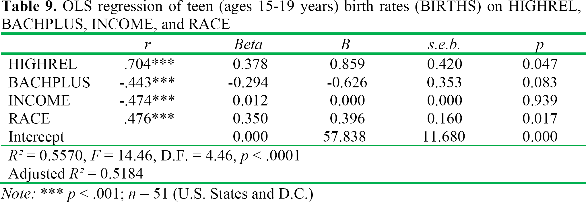
OLS regression of teen (ages 15–19 years) birth rates (BIRTHS) on HIGHREL, BACHPLUS, INCOME, and RACE
Note:
p < .001; n = 51 (U.S. States and D.C.)
The statistically significant and large positive correlation between HIGHREL and BIRTHS, along with the associated OLS regression analysis results, demonstrate the substantial explanatory power of HIGHREL regarding BIRTHS. At the same time, however, the coefficients and regression statistics for BACHPLUS and RACE reveal their separate contributions to explained variance. The higher the religiosity, the higher the teen birth rate. The lower the educational attainment, the higher the teen birth rate. The higher the percentage of African Americans, the higher the teen birth rate.
Health and morbidity
Data compiled by the OECD (Organization for Economic Co-operation and Development), reveal that the United States, despite its enormous wealth, scores lower than many or most member countries on virtually all indicators of health and morbidity (OECD, 2009). For example, in the years 2005–2006, the adult obesity rate in the U.S. was 34%, the highest among all 26 OECD nations for which obesity data were available. In contrast, Mexico's obesity rate was 30%, Canada's 15%, Netherlands 11%, and Japan 3%. Similarly, the U.S. ranked high in the prevalence estimates of chronic disease related to lifestyle, such as diabetes. For adults aged 20–79 years in 2010, the estimated diabetes rate for the U.S. was 10.3%, as compared to the OECD average of 6.3%. Only Mexico, at 10.8%, was higher than the U.S., with Greece, Italy, Ireland, Japan, United Kingdom, and Iceland at 6.0%, 5.9%, 5.2%, 5.0%, 3.6%, and 1.6%, respectively.
The “Overall Health” composite variable (United Health Foundation, 2009) includes a variety of measures of state health in 2007 and incorporates them into a combined indicator, which is the standardized z score, calculated as [(the state value of the composite measure – the national mean) ÷ the standard deviation of all state values]. The core measures comprising the composite include such “Behaviors” as prevalence of obesity, smoking, and binge drinking; “Community and Environment” factors, such as occupational fatalities per 100,000 workers, infectious disease per 100,000 population, air pollution (“micrograms of fine particles per cubic meter”), and percent of children in poverty; “Public and Health Policies,” focused on percent of the population without health insurance, immunization coverage, and public health funding; “Clinical Care,” such as prenatal care, preventable hospitalization, and number of primary care physicians per 100,000 population; and the “Health Outcomes” of premature death (“years lost per 100,000 population”), poor physical health days (“in the previous 30 days”), infant mortality, poor mental health days, cancer deaths, and cardiovascular deaths, each calculated per 100,000 population.
The z scores representing state values on this composite measure range from a low of −15.2 for Louisiana to a high of +24.8 for Vermont. The scores of the remaining New England states are 19.9 for New Hampshire, 17.7 for Massachusetts, 17.5 for Connecticut, Maine at 15.3, and Rhode Island at 14.0. Scores for the six states closest to Louisiana in overall health are Mississippi at −15.0, South Carolina −10.0, Tennessee at −9.7. Texas at −9.0, Florida at −8.9, and Oklahoma and Alabama, tied at −8.1 standard deviation units below the mean for all states.
As shown in Table 10, the significant and large positive correlation between HIGHREL and OBESITY along with the accompanying regression statistics indicate that HIGHREL accounts for or explains a substantial amount of variation in OBESITY. The same is true for BACHPLUS and RACE, however, and taken together, the independent variables of this analysis account for over 70% of the variation in adult obesity rates. The higher the religiosity, the higher the adult obesity rate. The lower the educational attainment, the higher the adult obesity rate. The higher the percentage of African Americans, the higher the adult obesity rate.
OLS regression of obesity rates (OBESITY) on HIGHREL, BACHPLUS, INCOME, and RACE

Note:
p < .001
p < .01; n = 51 (U.S. States and D.C.)
OLS regression of smoking rates (SMOKRATE) on HIGHREL, BACHPLUS, INCOME, and RACE

Note:
p < .001; n = 51 (U.S. States and D.C.)
Taken alone, the correlation between HIGHREL and SMOKRATE indicates a large positive relationship between the variables. The regression analysis results tell a different story, however, with the Beta, B, s.e.b., and p values showing that relationship largely to be spurious. The findings reveal that BACHPLUS and INCOME, with large negative correlations, are the best predictors of SMOKRATE. The lower the level of educational attainment within states, the higher the smoking rate, and the lower the median household income, the higher the smoking rate.
As shown in Table 12, the significant correlation indicates a moderate negative relationship between HIGHREL and ALCHONS and the corresponding regression Beta, B, s.e.b., and p values show that the relationship is not a spurious one. The higher the religiosity, the lower the alcohol consumption.
OLS regression of alcohol consumption (ages 14+ years) (ALCHONS) on HIGHREL, BACHPLUS, INCOME, and RACE

Note:
p < .001
p < .01
p < .05; n = 51 (U.S. States and D.C.)
OLS regression of overall health (HEALTH) on HIGHREL, BACHPLUS, INCOME, and RACE

Note:
p < .001; n = 51 (U.S. States and D.C.)
While the significant correlation of −.723 indicates a large negative relationship between HIGHREL and HEALTH, the accompanying results of the OLS regression analysis show that the relationship is largely spurious. It is BACHPLUS and RACE, with significant correlations with HEALTH of .648 and −.678, respectively, that account for the greatest amount variation in the overall health of state populations. The lower the level of educational attainment within states, the lower the level of overall health, and the higher the percentage of African Americans within states, the lower the overall health.
Mortality
“Mortality” is the final category of societal health indicators considered in the current study. It includes the “Infant Mortality Rate,” “Life Expectancy,” and the “Suicide Rate.” According to OECD Health Data for 2009, “Infant mortality has decreased sharply in OECD countries, associated with improvements in socio-economic status and health care” (OECD, 2009). Between 1970 and 2009, the average infant mortality rate for OECD nations declined from about 28 to about 5. The comparable figures for the U.S. were 20 in 1970 and 4.3 in 2009, below the OECD average at the earlier date and also below the OECD average recently. Comparable rates in 1970 and 2009 for Canada and Sweden were about 18 vs. 5 for Canada and 12 vs. 2.5 for Sweden. Within the U.S., the state-level infant mortality rates range from a low of 4.5 for Utah to a high of 14.1 for the District of Columbia (U.S. Census Bureau, 2005).
In 2007, Japan had the highest life expectancy at 82.6 years, compared with 78.1 for the U.S., which was also below the OECD average of 79.1 (OECD 2009). Only the Czech Republic, Poland, Mexico, the Slovak Republic, Hungary and Turkey, among the OECD countries, had life expectancies less than the U.S., the lowest being 73.2. By comparison, the life expectancy for the United Kingdom was 79.5, Germany 80.0, Canada 80.7, France 81.0, and Switzerland 81.9.
Among the OECD countries, the suicide rate for the U.S. fares better comparatively than does life expectancy (World Health Organization, 2008). For 2005, the U.S. suicide rate (suicides per 100,000 population) was 11.0, compared with Canada's 11.3, Germany's 11.9, Sweden's 13.2, France's 17.0, and Japan's 24.4. Suicide rates lower than that of the U.S. were observed in Ireland 9.7, Spain 7.8, Italy 7.1, United Kingdom 6.7, and Mexico 4.1.
OLS regression of infant mortality rate (INFANMOR) on HIGHREL, BACHPLUS, INCOME, and RACE

Note:
p < .001; n = 51 (U.S. States and D.C.)
The significant correlation between HIGHREL and INFANMOR indicates a large positive relationship between the variables, but the corresponding OLS regression statistics reveal that HIGHREL explains little of the variation in INFANMOR and the correlational relationship is spurious. In this analysis, it is RACE that has the greatest predictive power, with an r of .736 and corresponding Beta of .700. Both BACHPLUS and INCOME, with correlations of −.537 and −.572, respectively, also account for a substantial amount of the variation in infant mortality rates. The higher the percentage of African Americans within states, the higher the infant mortality rate. The lower the level of educational attainment and the lower the median family income, the higher the infant mortality rate.
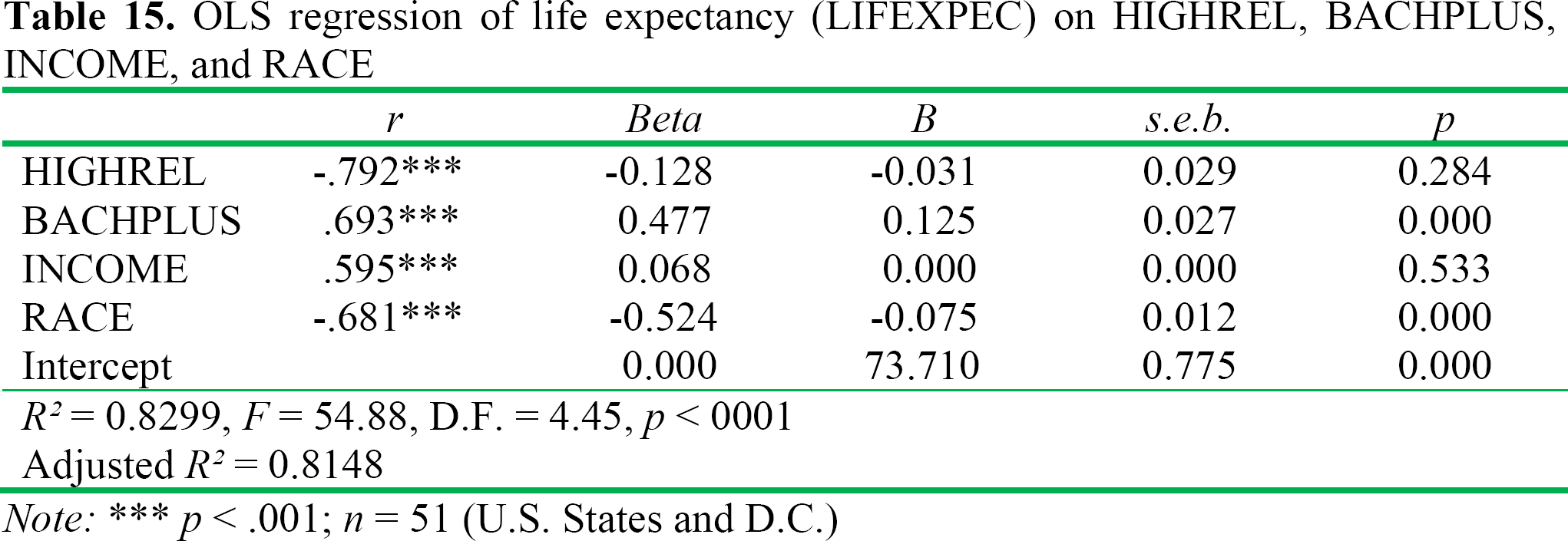
As displayed in Table 15, although the OLS regression analysis shows a p > .05, the large value of Beta suggests that the negative relationship between HIGHREL and LIFEXPEC may not be entirely spurious. Nonetheless, the corresponding robust positive correlations for BACHPLUS and RACE, respectively, demonstrate the more substantial power of these variables in accounting for variation in life expectancy in the U.S. The higher the educational attainment within states, the higher the life expectancy. The higher the percentage of African Americans within states, the lower the life expectancy.
OLS regression of life expectancy (LIFEXPEC) on HIGHREL, BACHPLUS, INCOME, and RACE
Note:
p < .001; n = 51 (U.S. States and D.C.)
Looking at Table 16, the correlation between HIGHREL and SUICIDE indicates but a small, non-significant positive relationship between the variables. The corresponding value of Beta shows that religiosity contributes little to explaining variation in suicide rates. In marked contrast are the negative correlation coefficients and substantial Beta values for BACHPLUS and RACE. The lower the level of educational attainment within states, the higher the suicide rate. The higher the percentage of African Americans within states, the lower the suicide rate.
OLS regression of suicide rates (SUICIDE) on HIGHREL, BACHPLUS, INCOME, and RACE

Note:
p < .001
p < .01; n = 51 (U.S. States and D.C.)
Part II
In this section, I present the results of 13 OLS regression analyses intended as partial tests of Paul's second major hypothesis that:
II. High levels of societal dysfunction contribute to the persistence of theistic beliefs and practices.
Whereas in Part I, the measure of high religiosity, HIGHREL, functioned as the primary independent variable, throughout this section it is the dependent variable in the analyses. In each OLS regression, BACHPLUS, INCOME and RACE serve as control variables, while the indicators of societal dysfunction that were the focus of Part I are treated as the principal independent variables. Table 17 examines the relationships between HIGHREL and the control variables only, while Tables 18–30 introduce, in turn, each of the indicators of societal dysfunction as independent variables.
OLS regression results for high religiosity (HIGHREL) regressed on educational attainment of bachelor's degree or higher (BACHPLUS), median household income (INCOME), and percent of African Americans (RACE)

Note:
p < .001; n = 51 (U.S. States and D.C.)
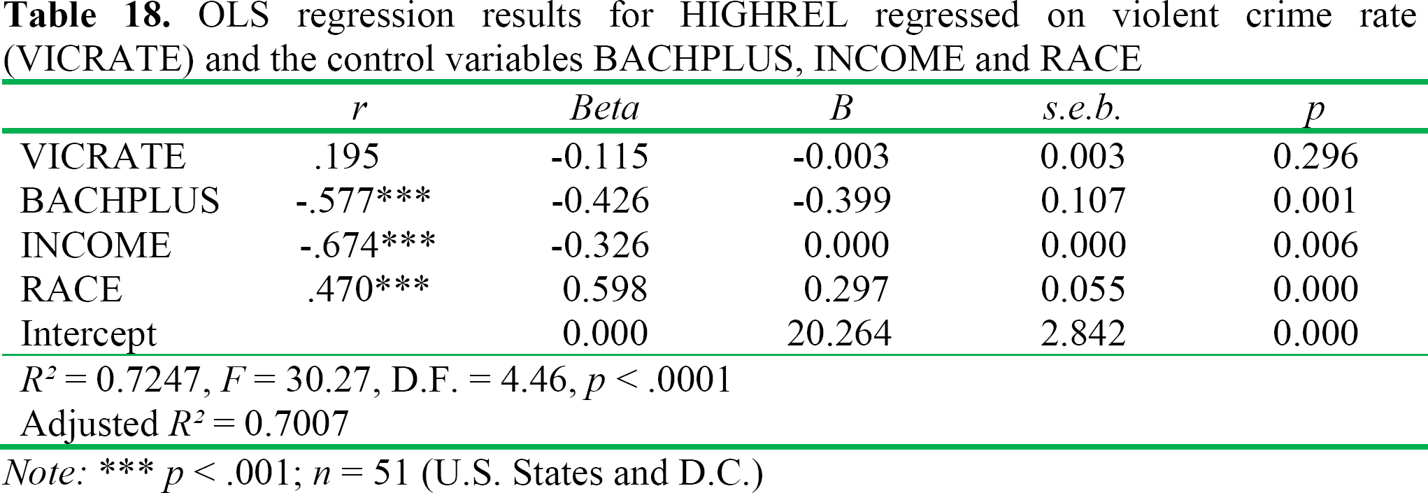
OLS regression results for HIGHREL regressed on violent crime rate (VICRATE) and the control variables BACHPLUS, INCOME and RACE
Note:
p < .001; n = 51 (U.S. States and D.C.)
OLS regression results for high HIGHREL regressed on murder rate (MURRATE) and the control variables BACHPLUS, INCOME and RACE

Note:
p < .001
p < .05; n = 51 (U.S. States and D.C.)
OLS regression results for HIGHREL regressed on incarceration rate (INCARATE) and the control variables BACHPLUS, INCOME and RACE

Note:
p < .001; n = 51 (U.S. States and D.C.)
OLS regression results for HIGHREL regressed on teen (ages 15–19 years) pregnancy rate (PREGRATE) and the control variables BACHPLUS, INCOME and RACE
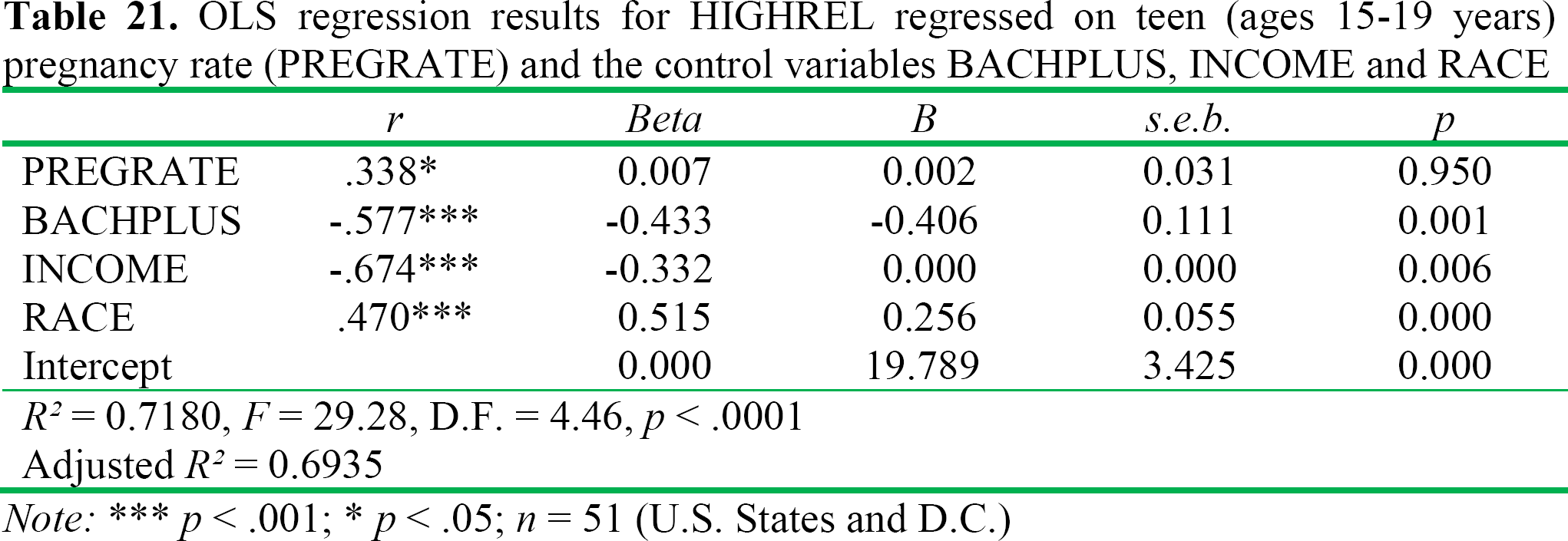
Note:
p < .001
p < .05; n = 51 (U.S. States and D.C.)
OLS regression results for HIGHREL regressed on teen (ages 15–19 years) abortion rate (ABORTIONS) and the control variables BACHPLUS, INCOME and RACE

Note:
p < .001
p < .01; n = 51 (U.S. States and D.C.)
OLS regression results for HIGHREL regressed on teen (ages 15–19 years) birth rate (BIRTHS) and the control variables BACHPLUS, INCOME and RACE

Note:
p < .001; n = 51 (U.S. States and D.C.)
OLS regression results for HIGHREL regressed on adult obesity rate (OBESITY) and the control variables BACHPLUS, INCOME and RACE

Note:
p < .001; n = 51 (U.S. States and D.C.)
OLS regression results for HIGHREL regressed on adult smoking rate (SMOKRATE) and the control variables BACHPLUS, INCOME and RACE

Note:
p < .001; n = 51 (U.S. States and D.C.)
OLS regression results for HIGHREL regressed on alcohol consumption (ages 14+) (ALCHONS) and the control variables BACHPLUS, INCOME and RACE

Note:
p < .001; n = 51 (U.S. States and D.C.)
OLS regression results for HIGHREL regressed on adult overall health (HEALTH) and the control variables BACHPLUS, INCOME and RACE
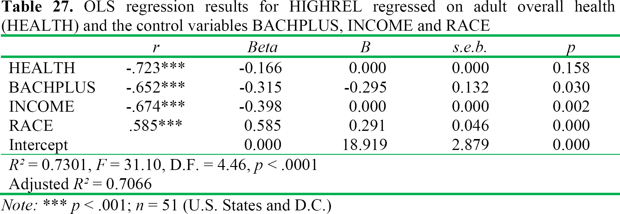
Note:
p < .001; n = 51 (U.S. States and D.C.)
OLS regression results for HIGHREL regressed on infant mortality rate (INFANMOR) and the control variables BACHPLUS, INCOME and RACE

Note:
p < .001; n = 51 (U.S. States and D.C.)
OLS regression results for HIGHREL regressed on life expectancy (LIFEXPEC) and the control variables BACHPLUS, INCOME and RACE
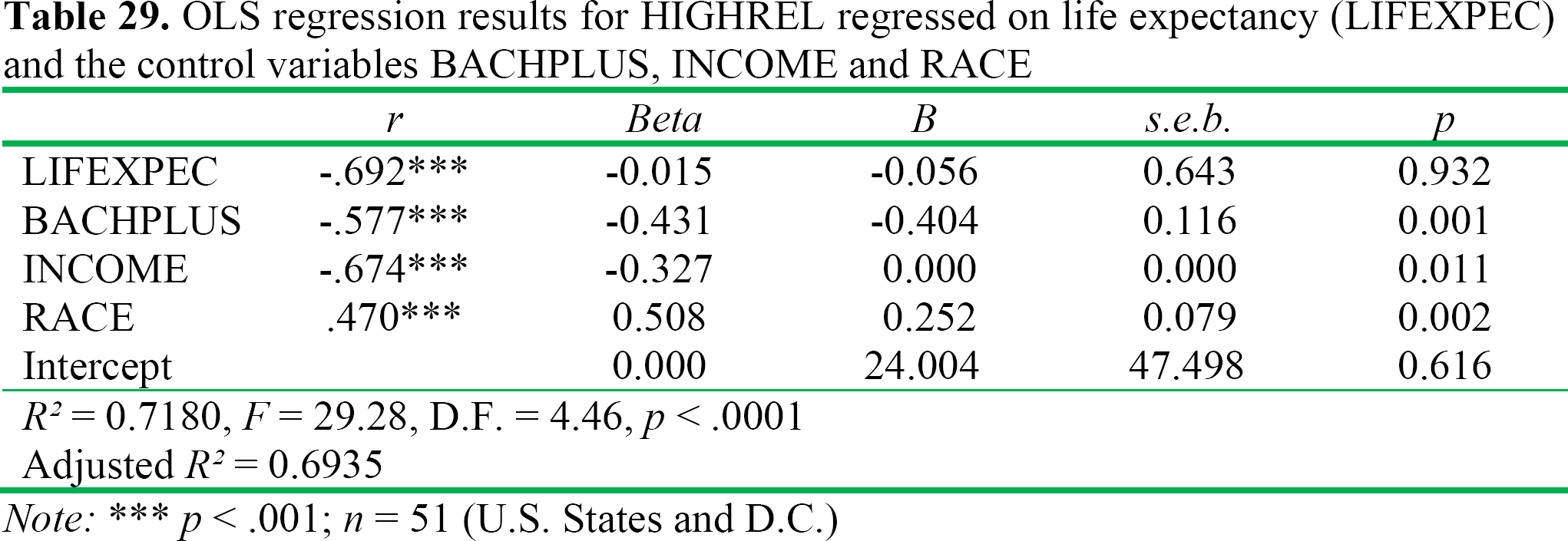
Note:
p < .001; n = 51 (U.S. States and D.C.)
OLS regression results for HIGHREL regressed on suicide rate (SUICIDE) and the control variables BACHPLUS, INCOME and RACE

Note:
p < .001; n = 51 (U.S. States and D.C.)
Looking at Table 20, compared with its relationships with either violent crime rates or murder rates, the large positive r of .613, together with the OLS results, suggest a notable degree of explanatory power for INCARATE as regards HIGHREL. Once again, however, the control variables, BACHPLUS, INCOME and RACE demonstrate the greatest predictability vis-à-vis religiosity. The higher the incarceration rate, the higher the religiosity. The lower the level of educational attainment and the lower the median household income, the higher the religiosity. The higher the percentage of African Americans, the higher the religiosity.
Taken together, these findings reveal the predictive power of BACHPLUS, INCOME, and RACE regarding HIGHREL, and collectively they account for over 70% of the variation in high religiosity. Furthermore, all of the VIF (Variance Inflation Factor) values (not displayed) are well below 5.0, indicating that multicollinearity is not an issue in this analysis. The lower the level of educational attainment, the higher the religiosity. The lower the median family income, the higher the religiosity. The higher the percentage of African Americans, the higher the religiosity.
As shown in Table 18, the low positive r value of .195, along with the values of B and s.e.b., indicate that the violent crime rate is not an important predictor of high religiosity. The three control variables are, however, with the greatest predictive power attributable to BACHPLUS and RACE. The lower the level of educational attainment, the higher the religiosity. The lower the median family income, the higher the religiosity. The higher the percentage of African Americans, the higher the religiosity.
While the statistically significant positive correlation of .274 suggests some effect of murder rates upon high religiosity (see Table 19), the results of the regression analysis point to the much greater explanatory power of the three control variables. The lower the level of educational attainment and the lower the median family income, the higher the religiosity. The higher the percentage of African Americans, the higher the religiosity.
Teen pregnancy rates, as evidenced particularly by the OLS regression results, appear to have a very small positive effect on religiosity of minor significance. Once Again, however, the predictive power of the control variables is primary, with BACHPLUS and INCOME associated with low levels of religiosity and RACE with high ones. The lower the level of educational attainment and the lower the median family income, the higher the religiosity. The higher the percentage of African Americans, the higher the religiosity.
As shown in Table 22, the teen abortion rate, as evidenced by the significant correlation of −.354, as well as by the accompanying OLS regression analysis statistics, explains a substantial amount of variation in levels of religiosity. The contributions of the control variables of BACHPLUS and, especially, RACE are more remarkable, however, continuing the pattern of observed relationships in the preceding regression analyses. The lower the abortion rate, the higher the religiosity. The lower the level of educational attainment and the lower the median household income, the higher the religiosity. The higher the percentage of African Americans, the higher the religiosity.
The correlation coefficients and regression analyses statistics shown in Table 23 suggest that a moderate amount of the variation in religiosity is accounted for by birth rates. The results again demonstrate the more substantial explanatory power of the control variables, however. The higher the birth rate, the higher the religiosity. The lower the level of educational attainment and the lower the median family income, the higher the religiosity. The higher the percentage of African Americans the, higher the religiosity.
According to the results of this OLS regression analysis displayed in Table 24, OBESITY, with its statistically significant large positive r of .771 and the accompanying regression statistics, is a strong predictor of religiosity. The predictive power of the control variables is also substantial, however. The higher the level of adult obesity within states, the higher the religiosity. The lower the level of educational attainment and the lower the median family income within states, the higher the religiosity. The higher the percentage of African Americans within states, the higher the religiosity.
Focusing only on the correlation between SMOKRATE and HIGHREL in Table 25 would suggest an apparent strong relationship between the variables. Examination of the results of the regression analysis leads to different conclusions, since the Beta, B, s.e.b., and p values suggest that the relationship is spurious. The relationships between SMOKRATE and the control variables appear to be real, however. The lower the level of educational attainment and the lower the median family income within states, the higher the religiosity. The higher the percentage of African Americans within states, the higher the religiosity.
The findings displayed in Table 26 indicate a moderate negative relationship between alcohol consumption and religiosity and the values of Beta, B, s.e.b., and p of the associated regression analysis indicate that this correlation coefficient value is not spurious. The control variables also make significant contributions to explained variance, which in this case is approximately 79% of religiosity. The lower the alcohol consumption within states, the higher the religiosity. The lower the level of educational attainment and the lower the median household income, the higher the religiosity. The higher the percentage of African Americans, the higher the religiosity.
The findings displayed in Table 27 include a strong negative relationship between the overall health of adults and the level of religiosity, and although the corresponding regression statistics are not significant at p < .05, the relationship does not appear to be wholly spurious. Nonetheless, and once again, the greatest predictive power comes from the control variables, especially RACE. The lower the overall health within states, the higher the religiosity. The lower the level of educational attainment and the lower the median family income within states, the higher the religiosity. The higher the percentage of African Americans within states, the higher the religiosity.
The significant positive correlation of .712 in column 1 of Table 28, while the highest among the four independent variables, is shown to be a probable spurious relationship between infant mortality rate and religiosity when the corresponding regression coefficients are considered. Higher levels of infant mortality apparently do not contribute to higher levels of religiosity. The same cannot be said of the control variables, however. Once again, we learn that the lower the level of educational attainment and the lower the median family income within states, the higher the religiosity; and the higher the percentage of African Americans within states, the higher the religiosity.
The correlational and OLS regression analysis results pertaining to life expectancy (see Table 29) mirror the results regarding the infant mortality rate. Again, the large correlation of the primary independent variable is demonstrated to be largely spurious, while the effects of the control variables are again significant. The lower the educational attainment and the lower the median family income, the higher the religiosity; and the higher the percentage of African Americans, the higher the religiosity.
The suicide rate apparently has no discernable effect upon level of religiosity, but the control variables do. The lower the level of educational attainment and the lower the median family income within states, the higher the religiosity. The higher the percentage of African Americans within states, the higher the religiosity.
Discussion
Parallel to the above description of the results, interpretation of the findings is organized into two sections, one for each of Paul's hypotheses pertaining to relationships between religiosity and societal dysfunction.
Part I. Hypothesis regarding the effects of religiosity on societal dysfunction: High levels of theism contribute to high levels of societal dysfunction.
A review of the results of the correlation and regression analyses show some support for the hypothesis. Religiosity is related to and contributes some degree of predictability regarding at least one indicator of societal dysfunction in each of the four categories. Specifically, we may assert that:
The higher the level of religiosity, the higher the incarceration rate.
The higher the level of religiosity, the lower the teen abortion rate.
The higher the level of religiosity, the higher the teen birth rate.
The higher the level of religiosity, the higher the adult obesity rate.
The higher the level of religiosity, the lower the alcohol consumption rate.
The higher the level of religiosity, the lower the life expectancy.
With the possible exception of the contributions of religiosity to lower levels of teen abortions and less alcohol consumption, high religiosity does appear to affect to some degree other indicators of societal dysfunction in the negative direction predicted by the hypothesis, namely, higher rates of incarceration, higher teen birth rates, higher adult obesity rates, and lower life expectancies.
Overall, however, the findings are indicative of much more robust relationships between the control variables of level of educational attainment, median family income, and percentage of African Americans, all of which contribute relatively more than religiosity to the explanation of the variation in the indicators of societal dysfunction:
The lower the level of educational attainment within states, the higher the level of societal dysfunction.
The lower the median family income within states, the higher the level of societal dysfunction.
The higher the percentage of African Americans within states, the higher the level of societal dysfunction.
Taken together, these findings suggest the greater dysfunctional effects of the system of social inequality in the United States, in comparison with the effects of high religiosity, regarding crime and punishment, teen reproductive behavior, health and morbidity, and mortality, and they are consistent with the reported results of previous studies cited in preceding sections.
What the control variables of education, income and race appear to have in common with religiosity is the relationships of each of the four with personal insecurity. It seems likely that low levels of education and income increase personal insecurity, as does being a member of the African American racial minority. The relationship between religiosity and personal insecurity is perhaps somewhat more problematic, since high religiosity may both decrease and increase personal insecurity. While denominational and non-denominational affiliations and religious beliefs and practices may operate to decrease personal insecurity, for some the belief in life after death and in both heaven and hell may be sources of anxieties leading to increased feelings of personal insecurity.
Catholics, for example, who believe that living a sin-free life, or at least confessing one's sins to a priest, increases the odds that they will go to heaven following death, may be more likely to experience feelings of personal insecurity, since there is always some likelihood that they could be sentenced to hell because of sinful behaviors. Individuals self-identifying with other denominations, such as Southern Baptists, believe that being baptized and accepting Jesus Christ as one's personal savior guarantee their ascension into heaven, and that may operate to increase feelings of personal security. An interesting analysis of the anxiety inducing existential dilemma regarding Pascal's wager as it relates to decision theory is examined in a recent article by Melkonyan and Pingle (2009).
Part II. Hypothesis on the effects of societal dysfunction on religiosity: High levels of societal dysfunction contribute to the persistence of theistic beliefs and practices.
In general, the current findings provide more support for this hypothesis than the one previously considered. While some of the relationships are not strong, nor the contributions to explained variance remarkable, I have found that within states:
The higher the violent crime rate, the higher the religiosity.
The higher the murder rate, the higher the religiosity.
The higher the incarceration rate, the higher the religiosity.
The lower the teen abortion rate, the higher the religiosity.
The higher the teen birth rate, the higher the religiosity.
The higher the level of adult obesity, the higher the religiosity.
The lower the alcohol consumption, the higher the religiosity.
The lower the overall health, the higher the religiosity.
As was the case regarding the first hypothesis, however, the explanatory power of the control variables of education, income and race vis-à-vis religiosity is more substantial than that of the primary independent variables of interest, in this instance those of societal dysfunction. In particular, i have discovered repeatedly that within states:
The lower the level of educational attainment, the higher the religiosity.
The lower the median family income, the higher the religiosity.
The higher the percentage of African Americans, the higher the religiosity.
These last three empirical generalizations are entirely consistent with the findings of Norris and Inglehart in their major comparative cross-national research as reported in their monograph, Sacred and Secular (2004). Like these researchers, I have found substantial support for the personal insecurity hypothesis of religiosity, namely, that: low levels of education, low levels of income, and membership in the African American racial minority contribute to personal insecurity which, in turn, apparently manifests itself in high levels of religiosity.
Summary and Conclusion
I have developed a novel composite measure of high religiosity that incorporates identification with the Evangelical Protestant tradition; belief in the absolute certainty that God exists; that the Bible is the actual word of God, literally true word for word; valuing religion as a very important part of everyday life; attending religious services at least once a week; and praying at least once a day. The operational definition of high religiosity corresponds closely with and receives validation from the belief in the “Type A-Authoritarian God,” as conceptualized, defined and utilized by Stark in his research on American Piety in the 21 st Century (2006).
The composite measure of high religiosity has been used to test the hypotheses involving the reciprocal relationships between high religiosity and levels of societal dysfunction that include 13 indicators of societal health subsumed within the categories of crime and punishment, teen reproductive behavior, health and morbidity, and mortality. Regarding Hypothesis I, that “High levels of theism contribute to high levels of societal dysfunction,” the results of correlational and OLS regression analyses provide only low to moderate support. On balance, the greater explanatory power of the social inequality variables of education, income, and race strongly suggests that “American Exceptionalism” among the 17 prosperous democracies in terms of its high levels of societal dysfunction is due more to its high degree of social inequality than to its high levels of theism, as compared with its modern industrial counterparts of the First World.
OECD data on the degree of income inequality are instructive in this regard. The “Gini Coefficient” is a measure of income inequality whose values range from a high of 1.0, where all of a nation's income is owned by one household or a small group of households, to a low of 0, where all income is shared equally among all households. The Gini Coefficient for the U.S. as a whole, as displayed in the United Nations' “2007/2008 Human Development Report,” was .40, as compared with the OECD total of .29, Canada with .27, France with .31, Germany at .27, Ireland at .28, Japan at .34, Sweden at .22, and United Kingdom at .27 (OECD, 2010).
The pattern of high income inequality in the U.S. is also indicated by another measure, namely, the top 20% to bottom 20% ratio. While that ratio in 2007/2008 for the U.S. was 8.4, indicating that the upper 20% earned 8.4 times more than the lower 20%, the comparable ratio for Canada was 5.5, for Sweden 4.0, Japan 3.4, France 5.6, United Kingdom 7.2, Germany 4.3, Norway 3.9, Australia 7.0, Switzerland 5.5, and Spain 6.0, for example. At 8.4, the U.S. is tied or nearly tied with Croatia 8.4, Ghana 8.2, Kenya 8.2 and the country of Georgia 8.3 (OECD, 2010).
As for Hypothesis II, “High levels of societal dysfunction contribute to the persistence of theistic beliefs and practices,” the current findings provide somewhat greater support. Once again, however, the social inequality variables of education, income, and race, as compared with several measures of societal dysfunction, explain most of the variation in levels of religiosity, and this is consistent with the personal insecurity hypothesis advanced by Norris and Inglehart (2004).
Confidence in these findings and associated theoretical implications must of necessity be modest cautious and modest, since our methodology, which utilizes state-level aggregate data pertaining to the U.S. States and the District of Columbia renders us susceptible to errors associated with the use of ecological units of analysis, especially the ecological fallacy. Additional research on this topic is warranted, ideally involving individuals as units of analysis, or at least ecological areas smaller in size and more demographically homogeneous than states.
Nevertheless, the current results suggest that “American Exceptionalism,” when defined as the unique coexistence of high theism and high societal dysfunction in the U.S. during the first decade of the Twenty-First Century, is best explained by its relatively high degree of social inequality, which contributes both to high levels of religiosity and societal dysfunction.
Footnotes
Acknowledgements
I am grateful to the editor and reviewers who provided several helpful suggestions for improving an earlier draft of this manuscript. Bill Miller, whose Open Stat online statistical package was utilized to perform all analyses in this study, was most generous in sharing his time and expertise to enhance my understanding of the relative advantages and disadvantages of the several multiple regression procedures available in Open Stat.
Appendix A. Variable names and definitions

| Variable Name | Definition |
|---|---|
| ABORTIONS. Abortion rates (abortions per 1,000) for women aged 15–19 years for the U.S. States and Washington, D.C. for the year 2000 (Guttmacher Institute, 2006). | |
|
|
|
| ABSCERT. Percentages of state populations responding that they were “absolutely certain” that God exists in response to the question “Do you believe in God or a universal spirit? [IF YES, ASK:] How certain are you about this belief? Are you absolutely certain, fairly certain, not too certain, or not at all certain?” in the 2007 Pew forum on Religion and Public Life U.S. Religious Landscape Survey. Includes Washington, D.C. (Pew, 2009). | |
|
|
|
| ALCHONS. Alcohol consumption rates (total per capita alcohol consumption in gallons of ethanol) for the U.S. States and Washington, D.C. (National Institute on Alcohol Abuse and Alcoholism of the National Institutes of Health, 2006). | |
|
|
|
| BIRTHS. Birth rates (births per 1,000) for women aged 15–19 years for the U.S. States and Washington, D.C. for the year 2000 (Guttmacher Institute, 2006). | |
|
|
|
| EVANPROT. Percentage of state populations self-identifying as Evangelical Protestants in the 2007 Pew Forum on Religion and Public Life U.S. Religious Landscape Survey. Includes Washington, D.C. (Pew, 2009). | |
|
|
|
| HEALTH. Overall health includes a variety of measures of State health combined into a composite indicator, a standardized z score, calculated as [(the state value of the composite measure - the national mean) ÷ the standard deviation for all state values]. (United Health Foundation, 2009). | |
|
|
|
| HIGHREL. Composite index calculated as the sum of the z scores for EVANPROT, ABSCERT, WORDGOD, VERYIMPO, SERVWEEK, and PRAYDAY. | |
|
|
|
| INCARATE. Inmates per 100,000 residents for each State and Washington, D.C. at mid-Year, 2005 (Bureau of Justice Statistics, 2008). | |
|
|
|
| INCOME. Median Household Income for each state plus Washington, D.C. (U.S. Census Bureau, 2008). | |
|
|
|
| INFANMOR. Number of infant deaths (aged 0–1 year) per 1,000 live births for the U.S. States and Washington, D.C. for the year 2005. (Centers for Disease Control and Prevention, 2005). | |
|
|
|
| LIFEXPEC. Average life expectancies from birth for the U.S. States and Washington, D.C. for the year 1999. (Harvard University School of Public Health, 2009). | |
|
|
|
| MURRATE. Homicides (including negligent manslaughter) per 100,000 population for each State and Washington, D.C. (U.S. Department of Justice, Federal Bureau of Investigation, 2006). | |
|
|
|
| OBESITY. Adult obesity rates, percent of obese adults (2007–2009 BMI average 30.0–99.8) for the U.S. States and Washington, D.C. (National Center for Chronic Disease and Health Promotion of the Centers for Disease Control, 2009). | |
|
|
|
| PRAYDAY. Percentage of state populations saying that they pray “at least once a day” in response to the survey question “People practice their religion in different ways. Outside of attending religious services, do you pray several times a day, once a day, a few times a week, once a week, a few times a month, seldom, or never?” in the 2007 Pew Forum on Religion and Public Life U.S. Religious Landscape Survey. Includes Washington, D.C. (Pew, 2009). | |
|
|
|
| PREGRATE. Pregnancy rates (pregnancies per 1,000) for women aged 15–19 years for the U.S. States and Washington, D.C. for the year 2000 (Guttmacher Institute, 2006). | |
|
|
|
| RACE. Percentages of state populations that are “Black or African American” for the year 2008. (U.S. Census Bureau, 2010). | |
|
|
|
| SERVWEEK. Percentage of state populations saying that they attend religious services “at least once a week” in response to the question “Aside from weddings and funerals, how often do you attend religious services: more than once a week, once a week, once or twice a month, a few times a year, seldom or never?” in the 2007 Pew Forum on Religion and Public Life U.S. Religious Landscape Survey. Includes Washington, D.C. (Pew, 2009). | |
|
|
|
| SMOKRATE. Percentage of State adult populations smoking cigarettes for the year 2009, (Behavioral Risk Factor Surveillance System of the Centers for Disease Control, 2009). Includes Washington, D.C. | |
|
|
|
| SUICIDE. Suicides per 100,000 population for the U.S. States and Washington, D.C. for the year 2006. (National Center for Health Statistics, 2006). | |
|
|
|
| VERYIMPO. Percentage of state populations saying that religion is “very important” in their lives in response to the survey question “How important is religion in your life: very important, somewhat important, not too important, or not at all important?” in the 2007 Pew Forum on Religion and Public Life U.S. Religious Landscape Survey. Includes Washington, D.C. (Pew, 2009). | |
|
|
|
| WORDGOD. Percentages of state populations responding that they believed that the Bible was the “actual word of God, literally true, word for word” in response to the survey question “Which comes closest to your view? [HOLY BOOK]* is the word of God, OR [HOLY BOOK]* is a book written by men and is not the word of God? [IF BELIEVE HOLY BOOK IS WORD OF GOD, ASK:] And would you say that the [HOLY BOOK]* is literally true word for word, OR not everything in [HOLY BOOK]* is to be taken literally, word for word?” in the 2007 Pew Forum on Religion and Public Life U.S. Religious Landscape Survey. Includes Washington, D.C. (Pew, 2009). | |
Note: For Christians and the unaffiliated, “the Bible” was inserted where indicated by [HOLY BOOK]; for Jews, “the Torah” was inserted; for Muslims, “the Koran” was inserted; for all other religious groups, “the Holy Scripture” was inserted.
Appendix B. Basic descriptive statistics for all variables

| ABORTIONS (n = 51) Mean = 20.510 Variance = 18.853 Std. Dev. = 4.342 |
| Std. Error of Mean = 1.527 .950 Confidence Interval for mean: 17.444 to 23.576 |
| Range = 49.000 Minimum = 6.000 Maximum = 55.000 Median = 17.000 |
| Q1 = 12.000 Q3 = 26.000 Interquartile range = 14.000 |
|
|
| ABSCERT (n = 51) Mean = 71.549 Variance = 77.293 Std. Dev. = 8.792 |
| Std. Error of Mean = 1.231 .950 Confidence Interval for mean: 69.076 to 74.022 |
| Range = 37.000 Minimum = 54.000 Maximum = 91.000 Median = 71.000 |
| Q1 = 64.000 Q3 = 79.000 Interquartile range = 15.000 |
|
|
| ALCHONS (n = 51) Mean = 2.443 Variance = 0.267 Std. Dev. = 0.516 |
| Std. Error of Mean = 0.072 .950 Confidence Interval for mean: 2.298 to 2.588 |
| Range = 2.880 Minimum = 1.340 Maximum = 4.220 Median = 2.360 |
| Q1 = 2.100 Q3 = 2.650 Interquartile range = 0.550 |
|
|
| BACHPLUS (n = 51) Mean = 27.612 Variance = 36.251 Std. Dev. = 6.021 |
| Std. Error of Mean = 0.843 .950 Confidence Interval for mean: 25.918 to 29.305 |
| Range = 33.200 Minimum = 15.900 Maximum = 49.100 Median = 26.700 |
| Q1 = 23.300 Q3 = 31.600 Interquartile range = 8.300 |
|
|
| BIRTHS (n = 51) Mean = 46.020 Variance = 164.620 Std. Dev. = 12.830 |
| Std. Error of Mean = 1.797 .950 Confidence Interval for mean: 42.411 to 49.628 |
| Range = 48.000 Minimum = 23.000 Maximum = 71.000 Median = 46.000 |
| Q1 = 35.000 Q3 = 59.000 Interquartile range = 24.000 |
|
|
| HEALTH (n = 50) Mean = 4.252 Variance = 107.814 Std. Dev. = 10.383 |
| Std. Error of Mean = 1.468 .950 Confidence Interval for mean: 1.301 to 7.203 |
| Range = 40.000 Minimum = −15.200 Maximum = 24.800 Median = 3.600 |
| Q1 = −4.925 Q3 = 12.125 Interquartile range = 17.050 |
|
|
| HIGHREL (n = 51) Mean = −0.000 Variance = 31.806 Std. Dev. = 5.640 |
| Std. Error of Mean = 0.790 .950 Confidence Interval for mean: −1.586 to 1.586 |
| Range = 23.452 Minimum = −9.885 Maximum = 13.567 Median = −1.181 |
| Q1 = −3.914 Q3 = 3.018 Interquartile range = 6.931 |
|
|
| INCARATE (n = 51) Mean = 628.686 Variance = 40994.5 Std. Dev. = 202.471 |
| Std. Error of Mean = 28.352 .950 Confidence Interval for mean: 571.740 to 685.633 |
| Range = 865.000 Minimum = 273.000 Maximum = 1138.000 Median = 636.000 |
| Q1 = 466.000 Q3 = 759.000 Interquartile range = 293.000 |
|
|
| INFANMOR (n = 51) Mean = 7.131 Variance = 3.034 |
| Std. Dev. = 1.742 Std. Error of Mean = 0.244 .950 Confidence Interval for mean: 6.641 to 7.621 |
| Range = 9.600 Minimum = 4.500 Maximum = 14.100 Median = 6.900 |
| Q1 = 5.900 Q3 = 8.000 Interquartile range = 2.100 |
|
|
| INCOME (n = 51) Mean = 50248.294 Variance = 65280361.052 Std. Dev. = 8079.626 |
| Std. Error of Mean = 1131.374 .950 Confidence Interval for mean: 47975.843 to 52520.745 |
| Range = 31742.000 Minimum = 36338.000 Maximum = 68080.000 Median = 48576.000 |
| Q1 = 43753.000 Q3 = 55109.000 Interquartile range = 11356.000 |
|
|
| LIFEXPEC (n = 51) Mean = 76.798 Variance = 2.316 Std. Dev. = 1.522 |
| Std. Error of Mean = 0.213 .950 Confidence Interval for mean: 76.370 to 77.226 |
| Range = 8.000 Minimum = 72.000 Maximum = 80.000 Median = 77.000 |
| Q1 = 75.800 Q3 = 77.900 Interquartile range = 2.100 |
|
|
| MURRATE (n = 51) Mean = 5.247 Variance = 18.113 Std. Dev. = 4.256 |
| Std. Error of Mean = 0.596 .950 Confidence Interval for mean: 4.050 to 6.444 |
| Range = 28.100 Minimum = 1.000 Maximum = 29.100 Median = 4.900 |
| Q1 = 2.500 Q3 = 6.800 Interquartile range = 4.300 |
|
|
| OBESITY (n = 51) Mean = 25.271 Variance = 8.309 Std. Dev. = 2.882 |
| Std. Error of Mean = 0.404 .950 Confidence Interval for mean: 24.460 to 26.081 |
| Range = 13.300 Minimum = 18.400 Maximum = 31.700 Median = 25.300 |
| Q1 = 23.300 Q3 = 27.400 Interquartile range = 4.100 |
|
|
| PRAYDAY (n = 51) Mean = 57.569 Variance = 82.970 Std. Dev. = 9.109 |
| Std. Error of Mean = 1.275 .950 Confidence Interval for mean: 55.007 to 60.131 |
| Range = 37.000 Minimum = 40.000 Maximum = 77.000 Median = 58.000 |
| Q1 = 52.000 Q3 = 66.000 Interquartile range = 14.000 |
|
|
| PREGRATE (n = 51) Mean = 77.843 Variance = 369.535 Std. Dev. = 19.223 |
| Std. Error of Mean = 2.692 .950 Confidence Interval for mean: 72.436 to 83.250 |
| Range = 86.000 Minimum = 42.000 Maximum = 128.000 Median = 76.000 |
| Q1 = 60.000 Q3 = 93.000 Interquartile range = 33.000 |
|
|
| RACE (n = 51) Mean = 11.378 Variance = 128.891 Std. Dev. = 11.353 |
| Std. Error of Mean = 1.590 .950 Confidence Interval for mean: 8.185 to 14.572 |
| Range = 54.600 Minimum = 0.600 Maximum = 55.200 Median = 7.700 |
| Q1 = 2.900 Q3 = 15.900 Interquartile range = 13.000 |
|
|
| SERVWEEK (n = 51) Mean = 38.941 Variance = 85.896 Std. Dev. = 9.268 |
| Std. Error of Mean = 1.298 .950 Confidence Interval for mean: 36.334 to 41.548 |
| Range = 38.000 Minimum = 22.000 Maximum = 60.000 Median = 38.000 |
| Q1 = 32.000 Q3 = 47.000 Interquartile range = 15.000 |
|
|
| SMOKRATE (n = 51) Mean = 20.057 Variance = 10.136 Std. Dev. = 3.184 |
| Std. Error of Mean = 0.446 .950 Confidence Interval for mean: 19.161 to 20.952 |
| Range = 16.600 Minimum = 11.700 Maximum = 28.300 Median = 19.800 |
| Q1 = 17.600 Q3 = 22.200 Interquartile range = 4.600 |
|
|
| SUICIDE (n = 51) Mean = 12.706 Variance = 11.715 Std. Dev. = 3.423 |
| Std Error of Mean = 0.479 .950 Confidence Interval for mean: 11.743 to 13.669 |
| Range = 15.800 Minimum = 6.800 Maximum = 22.600 Median = 12.100 |
| Q1 = 10.800 Q3 = 14.800 Interquartile range = 4.000 |
|
|
| VERYIMPO (n = 51) Mean = 55.627 Variance = 114.998 Std. Dev. = 10.724 |
| Std. Error of Mean = 1.502 .950 Confidence Interval for mean: 52.611 to 58.644 |
| Range = 46.000 Minimum = 36.000 Maximum = 82.000 Median = 55.000 |
| Q1 = 47.000 Q3 = 61.000 Interquartile range = 14.000 |
|
|
| VICRATE (n = 51) Mean = 431.61 Variance = 56804.08 Std. Dev. = 238.336 |
| Std. Error of Mean = 33.374 .950 Confidence Interval for mean: 364.574 to 498.642 |
| Range = 1392.000 Minimum = 116.000 Maximum = 1508.000 Median = 392.000 |
| Q1 = 280.000 Q3 = 546.000 Interquartile range = 266.000 |
|
|
| WORDGOD (n = 51) Mean = 32.863 Variance = 123.761 Std. Dev. = 11.125 |
| Std. Error of Mean = 1.558 .950 Confidence Interval for mean: 29.734 to 35.992 |
| Range = 48.000 Minimum = 16.000 Maximum = 64.000 Median = 31.000 |
| Q1 = 26.000 Q3 = 37.000 Interquartile range = 11.000 |