
Abstract
We present an approach for modelling heterogeneous gas flow patterns in gas transmission networks based on mixtures of generalized nonlinear models (GNMs). This enables the use of a gamma distribution for the dependent variable and to incorporate standard loading profile specifications based on nonlinear functions where the specific form to be used is explicitly prescribed by a regulatory framework agreement. We focus in particular on the modelling of the maximum daily gas flow to predict gas flow at low temperatures where we take into account if the weekday is a working day or a non-working day. The application to a gas flow dataset from Western Austria exemplifies the benefits of using mixture models to obtain maximum gas flow predictions while taking day characteristics into account.
Introduction
Maximum daily gas flow data typically exhibit a nonlinear decreasing consumption pattern subject to the outside temperature and a regulatory framework agreement explicitly prescribes the use of specific nonlinear regression functions as standard loading profiles for modelling these data. In addition, heterogeneity in these standard loading profiles is usually observable, for example, in relation to certain day-specific characteristics. With the maximum daily gas flow data being assumed to follow a gamma distribution, overall a mixture of generalized nonlinear models (GNMs) emerges as a suitable model class. A key aspect of the determination and balancing of gas flow is to predict the maximum daily amount of gas flow for low temperatures. For these temperatures, the data are typically sparse. In addition very low temperatures, which are even beyond the usual observation range for outside temperatures, are of particular interest and are referred to as design temperatures.
We propose mixtures of GNMs as a suitable and flexible model class in order to predict the required gas supply for design temperatures. Mixture models are a flexible model class where different component models can be easily included to adapt to specific data structures or modelling needs (e.g., Willemsen et al., 2017). Our proposed approach pre-specifies the nonlinear relationship in the components of the mixture in contrast to other mixture approaches where semi-parametric regression models are used for the components to capture nonlinearities (e.g., Meyer et al., 2024). Pursuing an approach where the nonlinear function is pre-specified is attractive due to the interpretability of the regression coefficients and hence can be found in different areas of applications.
We conjecture that one main driver for heterogeneity in gas consumption data is given by the information on working days and non-working days. Therefore, including this information in the model is crucial and we will outline and investigate different approaches for the incorporation of the indicator on working days and non-working days within the mixture model framework.
The natural nonlinear shape of gas flow motivates the use of a sigmoid regression function as basic framework for standard loading profiles. In addition, the specific form of these standard loading profiles is prescribed as part of the framework agreement for German operators of gas supply networks provided by the (BDEW, Bundesverband der Energie- und Wasserwirtschaft; see BDEW, 2021). Gas suppliers rely on suitable estimates of these synthetic standard loading profiles for the allocation of gas data as they enable the prediction of gas consumption in gas transmission networks. Detailed research on the functional structure is discussed by Hellwig (2003), BDEW (2021) and Koch et al. (2015). The application of the sigmoid function was also studied for the Austrian market by Almbauer (2008). In addition, Friedl et al. (2012) studied historical data of gas consumption for a gas supplier with the aim to improve gas supply and reduce operational costs using also this functional structure, providing explanations for its use. A crucial criterion for a suitable model was the reliable gas supply prediction of the maximum gas transportation for design temperatures. Following Friedl et al. (2012), we will concentrate on the modelling of the maximum daily gas flow based on daily mean temperatures and the information on working days and non-working days as this is of particular interest when assessing gas transportation capacity. We also employ the sigmoid function prescribed within the framework of the respective regulations (Friedl et al., 2012; BDEW, 2021).
Our study contributes in the following two ways to the existing modelling framework for gas flow considered in Friedl et al. (2012): (a) We consider the gamma distribution in order to model the daily maximum gas flow and (b) we incorporate heterogeneous patterns using the flexible mixture modelling framework. We address the inclusion of working days and non-working days as predictor variable within the sigmoid function and as concomitant variable in the model where we realize the full potential of mixture model-based clustering. We apply an efficient fitting algorithm for mixtures of several sigmoid models provided by the add-on software package flexmixNL for the R environment for statistical computing and graphics (see Omerovic, 2019a; Omerovic et al., 2022). This R package represents an extension of the well-known package flexmix (see Leisch, 2004; Grün and Leisch, 2007, 2008). Various other statistical applications make use of sophisticated mixture models building on flexmix (e.g., Grün and Hornik, 2012) and concomitant variable models (e.g., Larson and Dinse, 1985). We focus specifically on the prediction for design, that is, low, temperature values. We derive the standard errors for these predictions based on the observed information matrix because the underlying EM algorithm does not automatically provide information on the variability of the parameter estimates. Further, we illustrate the use of localized versions of information criteria such as AIC (Akaike Information Criterion) and BIC (Bayesian Information Criterion) for model selection to emphasize the focus on obtaining a good fit for design temperatures.
The article is organized as follows: The class of mixtures of GNMs proposed for flexible modelling of maximum daily gas flow building on the prescribed standard gas loading profile model is specified in Section 2. The underlying fitting algorithm is the EM algorithm which we briefly describe in Section 3. There we further outline the computation of standard errors and the derivation of confidence intervals for predicted mean values at design temperatures which are of crucial interest in this application. Section 4 presents the computational environment provided by the R package flexmixNL. Section 5 provides a simulation study to assess the performance of the proposed methodology on synthetic data. Section 6 discusses the application of the proposed mixture model class to gas flow data from Western Austria. Section 7 concludes.
Model specification
We consider finite mixtures of regression models consisting of K components. The response y denotes the standardized, that is, scaled by the overall empirical mean, maximum daily gas flow and is assumed to be drawn conditional on the predictor variables x and the concomitant variables w from the K-component mixture distribution given by

In this marginal specification the number of components K is considered to be fixed and the component-specific probability density function (PDF) f(y; μ(x, βk), ϕk) is supposed to be a member of the linear exponential family that differs across components solely in the parameters βk and ϕk. The component sizes πk are not only assumed to be positive and sum to one, but also to depend on the concomitant variables w through a concomitant variable model.
To model the standardized daily maximum gas flow, we consider gamma components, that is,

where the shape parameter corresponds to the dispersion parameter through νk = 1/ϕk and a nonlinear mean function μ(x, βk) > 0 is assumed for the response y > 0. This framework for the components corresponds to the model class of generalized nonlinear models (GNM; Wei, 1998; Turner and Firth, 2018). Gamma components are a natural choice for modelling standardized daily maximum gas flow because they naturally take into account that the dependent variable is positive and has a higher variance for higher mean values resulting in a parsimonious specification capturing this characteristic. For the gamma distribution the variance in the kth component equals μ(x, βk)2/νk.
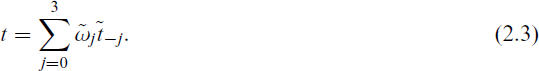
The mean μ(x, βk) depends on predictor variables x with component-specific parameters βk and follows the standard gas loading profile (BDEW, 2021). This profile has an underlying sigmoid functional structure which induces a decreasing consumption behaviour for increasing outside temperature. Following BDEW (2021), we take into account that the buildings’ heat accumulation capacity contributes to the daily gas consumption and use a weighted 4-day mean temperature as predictor variable instead of the respective single daily mean temperature. This weighted 4-day mean is determined with weights
The variables
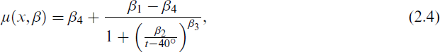
with predictor variable x = t.
The regression coefficients have the following physical meaning: Coefficients β1 and β4 describe upper and lower horizontal asymptotes of the sigmoid curve with β1 > β4, while β2 and β3 affect the shape and decrease of the curve with increasing temperature values. According to the energy industry, these parameters can be interpreted in the following way: The lower bound β4 incorporates a constant share of energy (warm water supply or share energy). The difference β1 − β4 indicates the decrease in gas consumption from cold to warm days. The coefficient β2 measures the change in gas consumption due to cold periods, while β3 refers to the dependence on the heating period. The temperature t is shifted by 40◦ to avoid discontinuities within the temperature range (Hellwig, 2003, p. 39).
As the prediction of the final gas flow is supposed to differentiate between working days and non-working days (see BDEW, 2021), we also include the indicator variable d in our model in order to denote whether or not the observation relates to a working day or a non-working day, respectively:
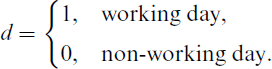
Non-working days refer in general to Saturdays, Sundays and public holidays.
The information on working days may be included in the model in different ways. The nonlinear regression function can be extended to include this variable by adding an additional parameter for working day and inserting this parameter in a specific way to alter the nonlinear function. Alternatively, this variable could also be seen as the main driver of heterogeneity and hence included to model the prior probabilities, that is, have the component weights vary with this indicator.
The first approach was considered in Friedl et al. (2012) in combination with a nonlinear regression model with normally distributed errors. They suggested to include this daily characteristic into the scope of the sigmoid regression function (2.4) by extending the functional form. They considered in particular the following specification:
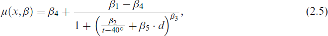
where the vector of regression coefficients is now given by β := (β1, β2, β3, β4, β5) and the predictor variables consist of the temperature t and the indicator d, that is, x = (t, d). Model (2.5) demonstrates that the additional information on the weekday influences the shape of the sigmoid curve rather than the constant share of energy β4 or the upper bound for daily gas consumption β1. This specification thus does not allow to capture a pattern where the gas consumption decreases on non-working days such that possibly also lower constant levels of energy shares are obtained. This would require varying regression coefficients β1 and β4.
As an alternative, we thus consider including the information on working days and non-working days as a concomitant variable within the mixture model framework allowing for different groups with varying regression parameters. The component weights may depend on α relating to the concomitant variables w where
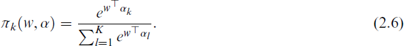
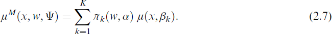
Model (2.1) is fully specified through the component weights, the component-specific mean functions and the dispersion parameters. In the following, we define the overall set of unknown parameters as Ψ = (π1, …, πK−1, β1, …, βK, ϕ1, …, ϕK) for mixtures without concomitant variables. For mixture models with concomitant variables, we replace π1, …, πK−1 with the parameter vector α. The marginal mean for given x and w is derived from (2.1) as
The main focus of the subsequent analysis lies in the estimation of the parameter vector Ψ and the prediction of the expected daily maximum gas flow for low temperature values while differentiating between working days and non-working days.
EM algorithm
For a sample of n observations the K-component mixture distribution in (2.1) yields the log likelihood function

with y = (yi)
i
=1,
…
,n, x = (xi)
i
=1,
…
,
n
and w = (wi)
i
=1,
…
,
n
. For the sake of convenience, we write fik = f(yi; μ(xi, βk), ϕk) for the PDF of the ith observation from the kth component. For mixture models, we assume the existence of heterogeneous discrete structures indicated by hidden or latent variables. Considering the latent variable z = (zik)
i
=1,
…
,
n
,
k
=1,
…
,
K
, we derive the complete-data log likelihood

where z consists of the component labels zik ∈ {0, 1} indicating the membership of the ith observation to the kth component. For mixture models the standard numerical approach to maximum likelihood estimation is based on maximizing the expected complete-data log likelihood function (3.2) through the EM algorithm. Given initial values, the EM algorithm constitutes an iterative two-step procedure executing an expectation- and a maximization-step. As the complete-data log likelihood ℓc(Ψ; y, x, w, z) depends on unknown information, we consider its conditional expectation given the observed data y, x and w and the current parameter estimate Ψ(
j
) in the jth iteration. Thus the E-step results in the objective function given by
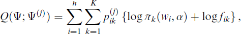
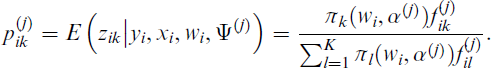
where the posterior weights
The updated parameter value Ψ( j +1) maximizes Q(Ψ; Ψ( j )) in Ψ for given Ψ( j ). In the case of mixtures of GNMs the mean function is given by a prespecified nonlinear regression function, as for example the sigmoid mean function in model (2.4) or (2.5) and the M-step requires an additional iteration loop in order to update the nonlinear regression parameters. As with one-component GNMs, convergence of the methods depends on a proper parameterization of the nonlinear mean function and the adequate choice of starting values. See Wei (1998) and Omerovic (2019a) for further details. We suggest a suitable initialization scheme for modelling standardized maximum daily gas flow in Section 5 where we also assess performance in a simulation study and subsequently make use of this initialization scheme in Section 6.
The two steps of the EM algorithm are iteratively repeated until a suitable stopping criterion is fulfilled. At convergence to a global maximum,
The EM algorithm does not automatically provide standard errors of the maximum likelihood estimator
where

O’Hagan et al. (2019) investigate the derivation of standard errors for Gaussian mixture models and point out that determining standard errors based on the Fisher information might give poor results for small sample sizes and unbalanced mixture component sizes. Similar findings are also reported recently in Griesbach and Hepp (2023). Both these contributions suggest to use suitable resampling methods to obtain standard error estimates. We investigate the suitability of the standard errors obtained using the Fisher information in the simulation study in Section 5 and find that their performance is satisfactory for the data scenarios considered which are similar to the setting in the empirical application. We thus conclude that resampling methods are not required in the empirical application to obtain reliable standard errors.
The use of mixtures of GNMs enables the prediction of gas flow while accounting for day characteristics in a flexible way. We use the mean of the maximum daily gas flow as determined conditional on x and w from the K-component mixture model (2.7). To also allow for the assessment of uncertainty associated with these point estimates, we construct confidence intervals for the predicted mean values.
The variance of the mean estimator μM(x, w,

where the gradient ∇(μM(x, w,

The gradient differs depending on the underlying mixture model (i.e., if constant component weights or a concomitant variable model are used) and on the number of unknown parameters in the nonlinear regression function. The standard error is determined by taking the square root, that is,

where zγ denotes the γ quantile of the standard normal distribution. The mean (2.7) and the interval (3.6) will be applied in the subsequent applications in order to predict the maximum daily gas flow for low temperatures and to assess the uncertainty associated with the prediction using confidence intervals.
The methods for estimation and inference are implemented in the R package flexmixNL (Omerovic, 2019b) which extends package flexmix (Leisch, 2004; Grün and Leisch, 2007, 2008). Package flexmix serves as the main base for the implementation by providing a generic infrastructure for the EM algorithm when fitting mixture models, exploiting that only slight adaptations of the EM algorithm need to be selectively implemented depending on the component-specific model used. Package flexmixNL extends these functionalities to be able to appropriately model mixtures of GNMs. It allows for the fitting of mixtures of GNMs with normal and gamma component distributions. Due to the nonlinearity of the mean functions, flexmixNL incorporates two crucial advancements: As the formula function may incorporate arbitrary nonlinear terms, flexmixNL takes this into account through the use of a symbolic language in the formula objects. Furthermore, the numerical procedures for the fitting of nonlinear functions afford the additional information on specific starting values which have to be provided for each component.
Technically, flexmixNL uses the functions nls() (for the normal distribution) and gnm() (for the gamma distribution) for fitting the component-specific parameters in the M-step. The latter belongs to package gnm introduced by Turner and Firth (2007). These fitting procedures have in common that they require appropriate starting values for all unknown regression coefficients in order to achieve convergent results. The starting values are provided through a list object when calling the fitting procedures. For a detailed explanation of the functionality and the technical architecture of flexmixNL see Omerovic (2019a) and Omerovic et al. (2022).
Predictions of mean values are derived through the evaluation of the marginal mean for the fitted mixture model at a specific predictor value, for example, a specific temperature value and day characteristic. Standard errors for
Simulation study for two-component mixtures
We analyze the performance of the fitting algorithm with a simulation study regarding parameter estimates and standard errors. The considered models are mixtures of GNMs consisting of two components with a gamma distributed dependent variable, the sigmoid mean function (2.4) and including a concomitant variable model. A key aspect of the simulation study is to assess how well the original configuration is reproduced and to analyze the discrepancy of the estimated parameters to the true values of the data generating process. We vary in particular the sample sizes to obtain insights on minimum required sample sizes to derive acceptable parameter estimates. Emphasis is also placed on performance assessment of the mean predictions, in particular for design temperatures. Our goal is to confirm that estimates with acceptable precision are delivered in order to substantiate the further modelling of the data from Western Austria.
Setup
The simulation study is based on a two-component gamma mixture model, that is,

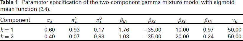
The component PDFs follow a gamma distribution (2.2) with shape parameter νk. The mean function corresponds to the sigmoid function (2.4) with temperature t as the sole predictor variable x. The indicator d for working days and non-working days is considered as concomitant variable w in model (2.6) for the prior probabilities. The regression coefficient vectors are given by βk = (βk1, βk2, βk3, βk4) for k = 1, 2. The specification of two components is inspired by the following scenario assumed for gas consumption: The first mixture component reflects the gas flow on days with consumption of industrial facilities in combination with households and the second component represents consumption at a lower level generated on days with essentially only private household consumption. The first component thus exhibits a higher consumption rate and has a greater component size. Due to the mean dependence of the variance for the gamma distribution, the variability increases with higher mean values yielding higher variability for the component including also the industrial consumption as the dispersion parameter is specified to be the same for both components.
Table 1 provides the complete parameter specification of the data generation process for model (5.1). These parameters induce that the component weight of the larger component of the working days and the non-working days is set to be 0.93 and 0.83, respectively. This is in line with the assumption that the prior probabilities
The differences between the component-specific values of the parameters βk1 and βk4 induce a gap between the upper and lower asymptotes thus enabling the modelling of two different consumption levels by means of a mixture distribution. Parameter βk3 has a significant influence on the decrease of the sigmoid mean function (2.4) for k = 1, 2. A central assumption in the construction of the synthetic dataset is that the parameters specified induce a mixture where the average maximum daily gas flow for one component is higher than for the other component across all temperature values. Such a setting also implies that the nonlinear mean functions are not supposed to cross. Therefore, the parameter specification in Table 1 induces a sharper decrease in consumption for the lower component. The parameters in Table 1 have been selected such that they are comparable to real world data (see Section 6). The predictor variables are drawn within the interval
Parameter specification of the two-component gamma mixture model with sigmoid mean function (2.4).
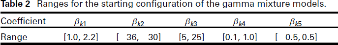
Ranges for the starting configuration of the gamma mixture models.
We summarize the results to assess the performance of mixture model parameter estimation using MC means, the bias (BIAS), the standard deviation (SD), the asymptotic standard errors (ASE) and the coverage rates (CR) at the confidence levels 95% and 99% for the concomitant variable model and the components of the two-component gamma mixture model (see Tables A.1, A.2 and A.3 in the supplementary material).
Overall the MC means
Predicting expected maximum gas flow values
We compute the MC means μM(xi, wi,
The SD are very close to the ASE and the confidence intervals show high congruence in general for the selected temperature values. The slightly increasing ranges for 15◦ and 25◦ are due to less data. Besides that, the confidence intervals of the mean values exhibit even wider ranges for low temperature values at −15◦ which coincides with the stronger variation of gas flow for low temperatures induced by the higher mean values.
Application to gas flow data in Western Austria
Data
The dataset combines information from three different sources to obtain data on gas flow, the daily mean temperatures and the type of day, that is, the working day indicators. Gas flow information is obtained for the market area Western Austria (Tyrol and Vorarlberg in Austria). The data are provided on the website of the Austrian balance group coordinators AGCS Gas Clearing and Settlement AG and can be accessed through
MC mean values evaluated at temperatures xi ∈ {−15, −10, −5, 0, 5, 10, 20, 25} with 95% confidence intervals based on standard deviations (SD) and asymptotic standard errors (ASE).
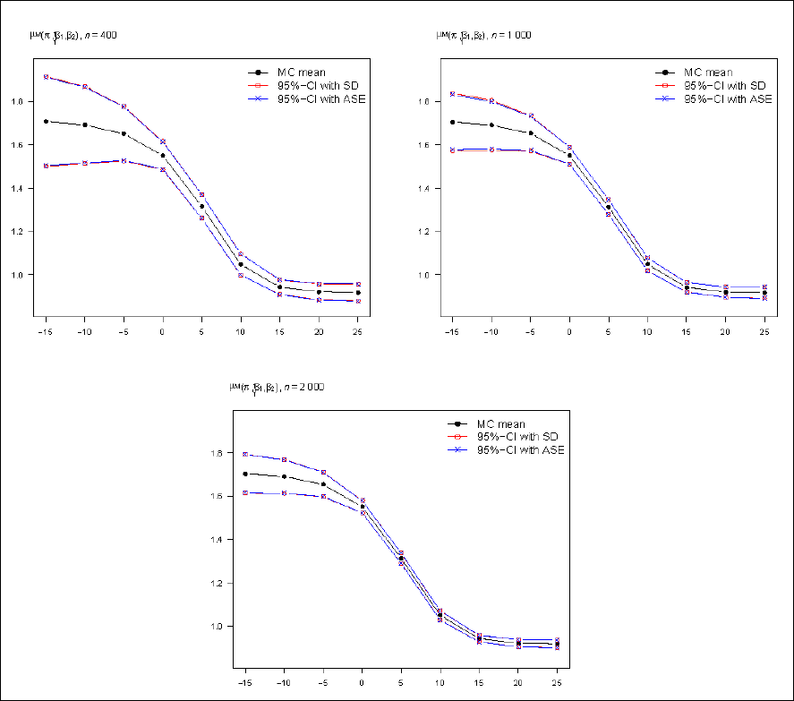
MC mean values evaluated at temperatures xi ∈ {−15, −10, −5, 0, 5, 10, 20, 25} with 95% confidence intervals based on standard deviations (SD) and asymptotic standard errors (ASE).
We derive the daily mean temperatures in degrees Celsius (◦C) from the Central Institution for Meteorology and Geodynamics (ZAMG, Zentralanstalt für Meteorologie und Geodynamik, recently renamed GeoSphere Austria) in Austria. We consider temperature values from a measuring station in Innsbruck (Austria, Tyrol) representative for the climate region of the gas distribution point for the gas flow data. The data can be accessed on the web page of ZAMG (2022). For the subsequent analysis we compute the weighted 4-day mean temperatures according to (2.3).
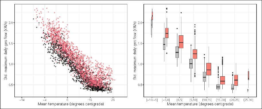
Maximum daily gas flow as scatter plot (left) and boxplot with binned temperature values (right) with distinction between non-working days (black) and working days (red).
We deduce the information on working days and non-working days based on the date stamp with the R package timeDate (Wuertz, 2018). We specify Saturday and Sunday to be non-working days and further add the information on national public holidays in Austria to also classify these days as non-working days. The remaining days are considered as working days.
The gas flow data is visualized in Figure 2. Working and non-working days are indicated by colour. Clearly there is a nonlinear relationship between temperature and gas flow visible with higher values for low temperatures, but a levelling off for high temperatures. The gas flow values are in general also higher for working than for non-working days regardless of the temperature. The data range considered implies that also observations from the COVID-19 pandemic are contained where official (mobility) restrictions were imposed. An exploratory analysis did not indicate an impact of COVID-2019 measures on the daily maximum gas flow, suggesting no need to account for COVID-19 lockdown periods. This analysis, however, provided strong evidence that warm temperatures during the winter months have an impact on the daily maximum gas flow re-confirming the need to include daily mean temperature as explanatory variable in the model.
In the subsequent analysis, we present the results for the two different possible model configurations to include the indicator d for working days and non-working days in the model. We either include this indicator with a regression coefficient in the nonlinear regression function or as a concomitant variable. Table 3 explains in detail how these specifications differ.
We first focus on comparing the one-component models resulting from these model configurations with the two-component mixture model extensions. The inclusion of two components is of particular interest as for the concomitant variable model this allows to assess congruence between the latent groups and the manifest working day indicator variable. The parameter estimates as well as their standard errors under all these models are reported and compared. In addition, for the concomitant variable model, the conditional prior probabilities for each component are determined in dependence of the working day indicator. The model fit is assessed and compared using different information criteria (AIC, BIC). We then also investigate the results when fitting mixtures with additional components. Finally, predictions of the mean values for low temperatures are obtained and compared for the selected models.
Model configurations of including the indicator di for working days and non-working days.
Model configurations of including the indicator di for working days and non-working days.
Models 1 and 2 with K = 1 and 2 were fitted with a set of 20 starting configurations with the starting values uniformly drawn from the ranges in Table 2. The ranges for the possible starting values are the same as used in the simulation study in Section 5, except that for this application now also an interval for βk5 is included. The length of the intervals are generously chosen to allow for identification of all potential solutions of the algorithm and select the best fitting one. Also these intervals have been shown to lead to reliable results in the simulation study. The results obtained are provided in Table 4.
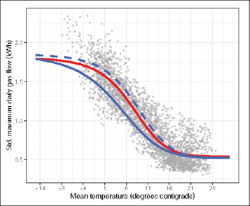
Figure 3 outlines the fitted regression functions for the one-component models, that is, where K = 1. Model 1 delivers results differentiating between working days (blue dashed line) and non-working days (blue solid line), whereas Model 2 results in a single sigmoid regression function (coloured in red). Model 1 indicates that the gas flow varies in its shape depending on if a day is a working or a non-working day. The gas flow declines faster on non-working days while it remains longer on a higher level on working days. Both functions converge to the approximately same constant gas flow level for temperatures beyond 16◦. Including an indicator for working days and non-working days influences the shape of the sigmoid regression curve while the asymptotes, reflected by the parameter estimates βˆ1 and βˆ4, remain almost unchanged for both models. Clearly both one-component models fail to provide different fitted values for working days compared to non-working days when considering high or low temperatures.
Figure 4 illustrates the fitted expected maximum daily gas flow functions of the two-component mixture models based on the marginal mean functions predicted for working days and non-working days. In Model 1 the working day indicator is included as a regression parameter. The marginal means are thus determined by summing over the two components using their prior weights πk and the component specific mean functions conditional on the day being a working day or a non-working day.
Parameter estimates with standard errors below.
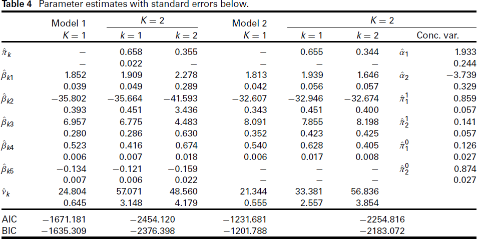
Parameter estimates with standard errors below.
Fitted one-component models for Model 1 (non-working days shown as solid blue line, working days shown as dashed blue line) and Model 2 (red solid line).
Including a concomitant variable model in Model 2 implies that the prior weights of the components vary between working days (w = 1) and non-working days (w = 0) based on (2.6). The coefficient of the concomitant variable model is reported in Table 4 and can be used to compute the expected gas flow based on the fitted component means and depending on if a day is a working day or a non-working day. On working days, the first (i.e., the upper) component accounts for about 85.9% (
Fitted marginal means (left Model 1, right Model 2) and observations coloured according to working days (red) and non-working days (blue).
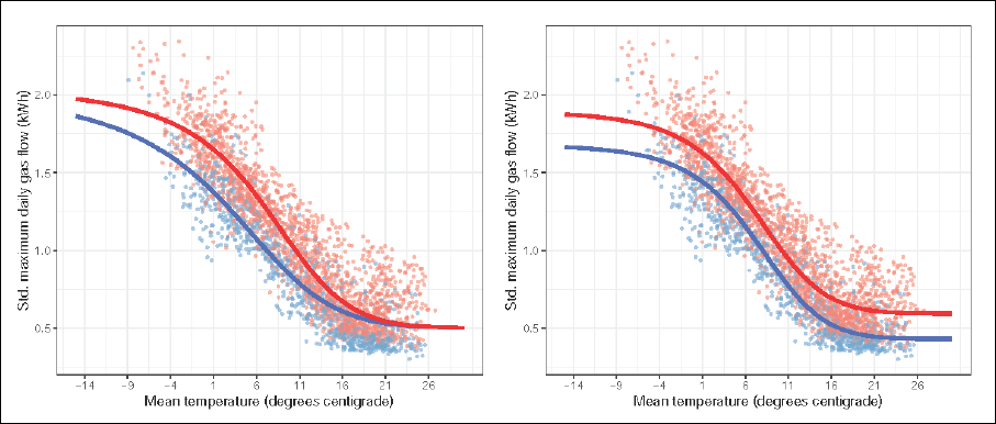
Both two-component models allow for a distinctly different fit between consumption on working days and non-working days. The two models differ, however, in particular in the fitted values of very low and very high temperatures. The marginal mean functions estimated under Model 1 suggest an intersection for low temperature values less than −15◦, as evident in Figure 4. By contrast, Model 2 gives two shifted mean functions allowing for a clear distinction in gas flow for the observed temperature values on working days and non-working days. This result supports the assumption of two distinct consumption levels for the whole temperature range depending on the day being a working day.
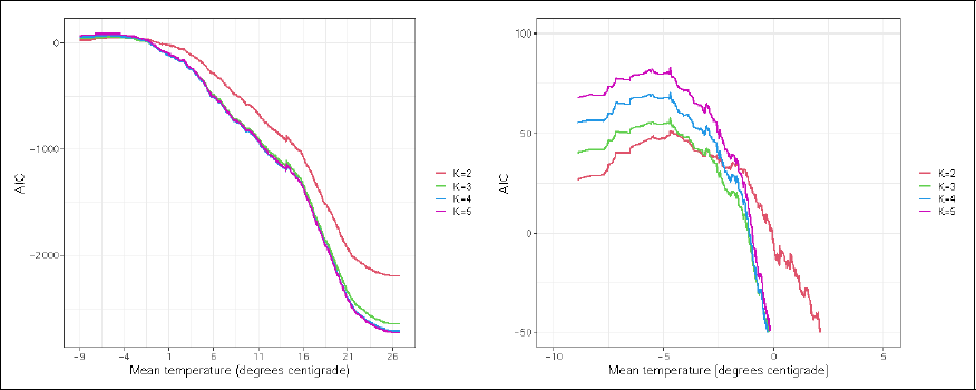
Using mixture models as modelling class allows fitting even more complex models by including additional components. We fit models up to the number of components K = 5 to the gas flow dataset and compare them through the model selection criteria based on AIC and BIC. AIC and BIC represent both global measures of goodness-of-fit. As the focus of our analysis lies on the balancing and prediction of gas flow for low temperatures (design temperatures), we use localized versions of the AIC and BIC in our model comparison which focus on obtaining a good fit for low temperatures. We determine the localized version of the AIC based on an increasing window along the temperature axis in order to assess the effect of considering an expanding range of temperatures on the model choice, that is,

with
The global AIC would suggest that the four- and five-component models result in the smallest, similar values. Focusing, however, on the localized version suggests that for temperatures below −5◦ the AIC selects the one-component configuration for Model 1. Regarding Model 2, the localized AIC prefers the two-component mixture model for temperatures below −5◦, given that we discard the one-component model from the consideration set as it does not allow to distinguish between working days and non-working days in prediction. The localized BIC results are comparable and would imply a similar model choice. Results are hence not shown. Clearly more parsimonious models are selected in case focus is only on the performance at low values compared to when the global performance is taken into account.
Localized AIC values for Model 1 and number of components between 1 and 5 (left entire temperature scale, right temperatures below 5◦).
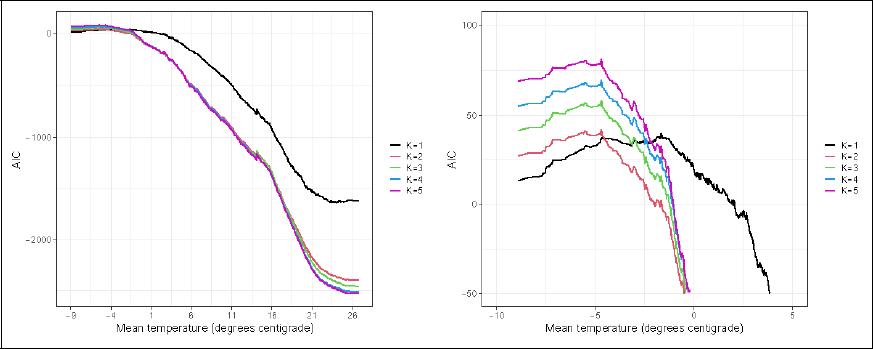
Localized AIC values for Model 2 and number of components between 2 and 5 (left entire temperature scale, right temperatures below 5◦).
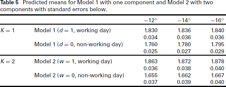
Final, we compute the predicted means of gas flow for temperature values ranging between −12◦ and −16◦. We restrict the models of interest to those preferred by the localized versions of AIC and BIC for low temperature values and which allow for a differentiation between working and non-working days: Model 1 with one component and Model 2 with two components. Table 5 displays the predicted mean values and their standard errors for the two models. We observe a stronger contrast between the predicted mean values for working days and non-working days under Model 2 compared to Model 1. This implies that Model 2 induces a stronger differentiation between working and non-working days, potentially leading to an improved estimate of the mean maximum daily gas flow for design temperatures.
Predicted means for Model 1 with one component and Model 2 with two components with standard errors below.
In this article, we presented a suitable approach for modelling the maximum daily gas flow depending on daily temperature values and an indicator for working days and non-working days. The presented approach is in particular suitable when dealing with heterogeneous data patterns which might occur due to different consumption levels entailed for example by working days and non-working days. The application of mixture models shows an improvement when predicting mean gas flow for low temperatures as it allows to differentiate between distinct components. We presented two approaches for the inclusion of such an indicator variable within the mixture model framework. Furthermore, we considered generalized nonlinear regression models for the mixture components using a gamma distribution for the dependent variable. The gamma distribution is particularly suited to model maximum daily gas flow because of the interdependence of the variability with the mean values. We validated the underlying estimation algorithm by means of a simulation study where we delivered parameter estimates and standard errors of acceptable precision. The new approach was applied to a real world data set for the Austrian market where we succeeded to identify several components based on implicit information in the data.
In our application we focused on a setting where the gas flow only for a single station was modelled in compliance with a regulatory agreement framework. Extensions could be considered for settings where several stations are included. In this case, a nonlinear mixed-effects approach (Pinheiro and Bates, 1995) could be employed to account for heterogeneity across stations and the inclusion of spatial information considered. In case modelling approaches not in line with the regulatory agreement framework are also to be considered, the use of generalized additive models such as GAMLSS (Rigby and Stasinopoulos, 2005) might seem appealing in order to account for the nonlinear shape in a data-driven way.
Footnotes
Acknowledgements
The authors would like to thank the anonymous referee and the associate editor for their helpful comments that improved the quality of the manuscript.
Declaration of Conflicting Interests
The authors declared no potential conflicts of interest with respect to the research, authorship and/or publication of this article.
Funding
The authors received no financial support for the research, authorship and/or publication of this article.
Supplemental material
References
Supplementary Material
Please find the following supplemental material available below.
For Open Access articles published under a Creative Commons License, all supplemental material carries the same license as the article it is associated with.
For non-Open Access articles published, all supplemental material carries a non-exclusive license, and permission requests for re-use of supplemental material or any part of supplemental material shall be sent directly to the copyright owner as specified in the copyright notice associated with the article.