
Abstract
Stepwise approaches for the estimation of latent variable models are becoming increasingly popular, both in the context of models for continuous (factor analysis and latent trait models) and discrete (latent class and latent profile models) latent variables. Examples include two-stage path analysis, structural-after-measurement and Croon’s bias-corrected estimation of structural equation models, and two- and three-step latent class and latent Markov modelling. These methods have in common that the measurement/clustering part of the model is estimated first, followed by the estimation of a—possibly complex—structural model. In this article, we review the existing approaches, which differ in how the information on the latent variable(s) is used when estimating the structural model. We show that based on these differences, stepwise latent variable modelling approaches can be classified into three main types: the fixed parameters, the single indicator and the bias adjustment approach. We discuss similarities and differences between these approaches, as well as between approaches proposed specifically for either continuous or discrete latent variables. Special attention is paid to heterogeneous measurement error resulting from missing data or measurement non-invariance, standard error estimation and software implementations.
Keywords
Introduction
Recently, we have seen a renewed interest in stepwise latent variable modelling approaches, which involve separating the estimation of the measurement and the structural parts of the model of interest. Examples for continuous latent variables include Structural After Measurement (SAM) estimation (Rosseel and Loh, 2024), two-stage path analysis (Lai and Hsiao, 2022), two-step latent trait modelling (Kuha and Bakk, 2023) and Measurement and Uncertainty Preserving ParamETric (MUPPET) modelling (Levy, 2023; Levy and McNeish, 2024). Similar approaches have been proposed for discrete latent variables, such as three-step latent class analysis (Bolck et al., 2004; Vermunt, 2010) and two-step latent class analysis (Bakk and Kuha, 2018).
Typically, two types of arguments are mentioned by authors contributing to the field of stepwise latent variable modelling; that is, arguments related to model estimation and to model building. Regarding model estimation, separate estimation of the measurement and the structural parameters yields fewer convergence problems is less affected by model misspecifications, and is computationally less demanding when dealing with large models (Bartolucci et al., 2015; Perez Alonso et al., 2024; Rosseel and Loh, 2024). In addition, stepwise model building, where one constructs measurements for the variables of interest and subsequently uses these to investigate their relationships, is also what most applied researchers prefer doing, among others to comply with the standard practice in their field, to prevent interpretational confounding, or to circumvent the need to remove cases with missing values on covariates (Burt, 1976; Vermunt, 2010; Clouth et al., 2022; Levy, 2023). Given that most researchers use such a strategy, stepwise latent variable modelling approaches have the potential to yield great improvement over naive use of estimated latent variable scores in subsequent analyses without accounting for their uncertainty (Rein et al., 2025).
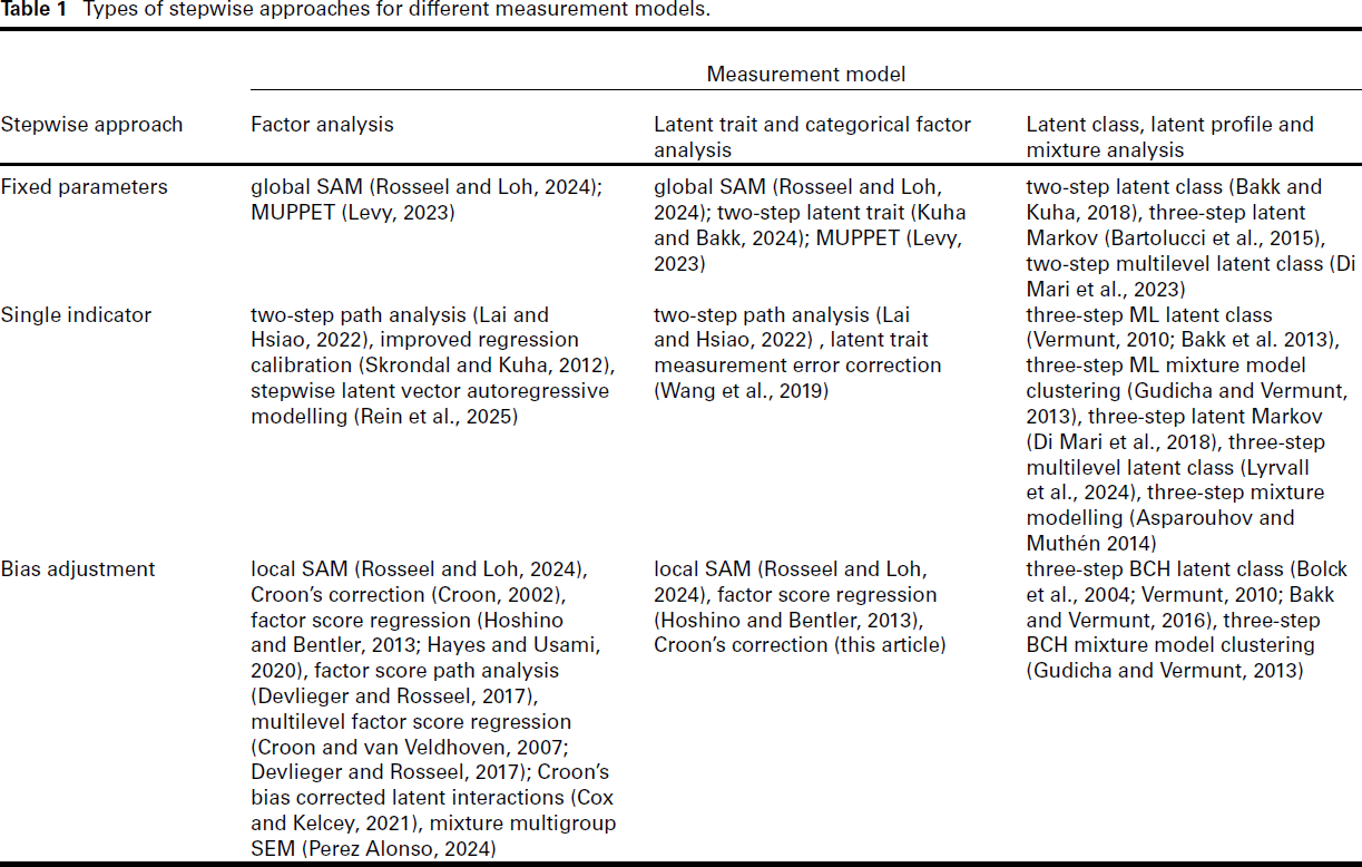
As shown in Table 1, stepwise approaches have been developed for each of the four types of latent variables models described by Lazarsfeld and Henry (1968) and Bartholomew and Knott (1999). These are (a) factor analytic models for continuous latent variables and continuous observed indicators, (b) latent trait models for continuous latent variables and discrete observed indicators, (c) latent profile models for discrete latent variables and continuous observed indicators and (d) latent class models for discrete latent variables and discrete observed indicators. Latent trait models are also referred to as item response theory (IRT) models or categorical factor analytic models, and latent profile and latent class models are also referred to as mixture models.
Types of stepwise approaches for different measurement models.
Types of stepwise approaches for different measurement models.
The structural models for which stepwise approaches have been developed are sometimes simple linear or logistic regression models in which a single latent variable serves as dependent or independent variable, but can also concern more complex models, such as path models containing multiple latent variables, latent Markov models or dynamic factor models for longitudinal data, or latent variable models for multilevel data.
Stepwise latent variable approaches appear in the literature under different names such as Structural After Measurement (SAM) estimation, two-stage analysis, two-step analysis, Croon’s bias-corrected estimation, Croon’s method and three-step analysis. However, the first step of all these approaches deals with the estimation of the measurement model for the latent variables without accounting for the structural model. The approaches differ from one another with respect to how the measurement model parameters are used when estimating the parameters of the structural model. Based on these differences, stepwise latent variable modelling approaches can be classified into three main types, which we will refer to as the fixed parameters, the single indicator and the bias adjustment approach. Table 1 lists the most important contributions to each of these.
In the fixed parameters approach, when estimating the parameters of the structural model, the measurement model parameters are fixed to the values obtained in the first step. Examples of this approach include Burt’s approach (Burt, 1976), global SAM estimation (Rosseel and Loh, 2024), two-step latent trait analysis (Kuha and Bakk, 2023), MUPPET modelling (Levy, 2023; Levy and McNeish, 2024), two-step latent class analysis (Bakk and Kuha, 2018) and three-step latent Markov modelling (Bartolucci et al., 2015).
The single-indicator approach involves obtaining predictions for the latent variables using the parameters of the measurement model. The predicted scores are used as single indicators when estimating the structural model, while accounting for their unreliability or misclassifications. This is a rather old idea within the SEM framework, and referred to as two-step SEM (Bollen, 1989). Lai and Hsiao (2022) showed how to use this approach when the measurement model is a latent trait model instead of factor analytic model, and refer to this approach as two-stage path analysis. Moreover, Lai et al. (2023) showed how to apply two-stage path analysis when there is measurement non-invariance. In the context of latent class and latent profile analysis, this approach was proposed by Vermunt (2010) and Gudicha and Vermunt (2012), who refer to it as three-step analysis with maximum likelihood adjustment for classification errors (see also Asparouhov and Muthén, 2014). Somewhat related single-indicator approaches have been proposed by Skrondal and Kuha (2012) and Savalei (2019).
The bias adjustment approach involves obtaining predictions for the latent variables using the parameters of the measurement model, and subsequently adjusting their covariances (or associations) so that these represent the true latent variable covariances. The adjusted covariances are used as if they were observed covariances when estimating the structural model parameters. This method was originally developed by Croon (2002) who derived the required adjustment for both factor analytic and latent class models (see also the related work by Wall and Amemiya, 2000). Devlieger and Rosseel (2017) used this approach in what they refer to as factor score path analysis. Although derived and implemented in a slightly different manner, the recently proposed local SAM approach by Rosseel and Loh (2024) can be seen as a special case of Croon’s method for continuous latent variables. Croon’s method for discrete latent variables was extended in various ways by Bolck et al. (2004), Vermunt (2010), Gudicha and Vermunt (2011), and Bakk et al. (2013), and is typically referred to as the Bolck-Croon-Hagenaars (BCH) approach.
The next three sections provide more details on the implementation of the three types of stepwise estimation methods with factor analytic models (Section 2), latent trait and categorical factor analytic models (Section 3), and latent class, latent profile and mixture models (Section 4). Subsequently, in Section 5, we discuss topics such as heterogeneous measurement error resulting from missing data or measurement non-invariance, standard error estimation and software implementations. We conclude with a short discussion in Section 6.
Background
Assuming the data are centred, and therefore ignoring the mean structure and representing the vector of latent variables by the vector η, the regression equations defining the measurement and structural parts of a structural equation model (SEM; Bollen, 1989) for the response vector 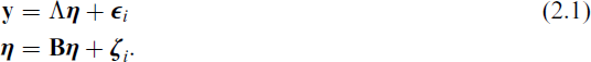
The free parameters are the factor loadings, residual covariances, regression coefficients and residual factor covariances, which are collected in the matrices Λ, Θ, 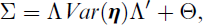
with

The various stepwise approaches have in common that they first estimate the measurement parameters Λ and Θ, while the structural parameters
Let 
or, equivalently,

Here Φ denotes the factor covariance matrix obtained from the measurement model. This yields modal a posteriori (MAP) or expected a posteriori (EAP) estimates of the factor scores. The posterior variance of the regression factor scores equals:

Maximum likelihood or Barlett factor scores (Barlett, 1938) are obtained with factor-score matrix

Instead of using a factor-score matrix based on the measurement model parameters, one may also use a simple sum score of the items as an estimate of the latent variable, in which case the factor-score matrix equals
To prevent what he refers to as interpretational confounding, Burt (1976) proposed estimating the measurement model separately for each latent factor, and subsequently estimating the structural model of interest with the measurement parameters—loadings and residual covariances—fixed. A similar but slightly more general fixed parameters approach was recently proposed by Rosseel and Loh (2024), who refer to it as global SAM estimation. An important difference is that global SAM was presented as an estimation method, whereas Burt presented his approach as a modelling method. In addition, the global SAM approach is more flexible in the sense that the measurement model may be estimated jointly for all latent variables, separately for each latent variable, or separately for blocks of latent variables. Moreover, the estimator used for the measurement model can differ from the one used for the structural model.
Another fixed measurement parameters approach called MUPPET modelling was proposed by Levy (2023), who also stressed the issue of interpretational confounding. MUPPET is a Bayesian two-step MCMC estimation approach for factor analytic models with covariates and outcome variables. The Bayesian estimation framework allows accounting for the uncertainty in the measurement parameters when estimating the structural parameters; that is, the saved draws of measurement model parameters from their posterior distribution are reused when drawing the structural parameters.
Single indicator
The single-indicator approach has been advocated among others by Lai and Hsiao (2022) who refer to it as two-stage path modelling. Rein et al. (2025) proposed using this approach in the context of latent vector autoregressive models for intensive longitudinal data subject to measurement error.
The single-indicator approach assumes that factor scores 
which shows how the factor scores are related to the true latent variable scores. Moreover, this equation demonstrates factor scores
The measurement model for the factor scores can also be written in terms of factor covariances, which yields

The reliability of the factor scores equals:

that is, the ratio between the (appropriately weighed) true and the estimated factor variance.
Let 
Using equation 2.7 for a single factor and noting that ϕ = var(η), we obtain
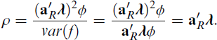
Multiply by ϕ/ϕ yields
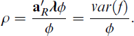
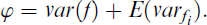
This shows the reliability of regression factor scores equals the ratio between the estimated and the true factor variance. Using this equation, the factor score variance var(f) can be decomposed as follows:

which is a special case of the more general equation 2.6, with
Another important characteristic of regression factor scores is that their true factor variances ϕ can be derived from the factor scores and their variances as follows:

where varf represents the posterior variance of the individual’s factor scores (see equation 2.3). Equation 2.9 follows from the definition of var(f) in equation 2.8 and the application of the definition in equation 2.3 to a single factor, which yields varf. Note that this equation is equivalent to the Expectation step for obtaining the expected factor covariance matrix when using the Expectation-Maximization algorithm for maximum likelihood factor analysis (Dempster et al., 1977).
In summary, stepwise SEM using regression factor scores as single indicators involves fixing their loadings and residual variances to ρ and ϕρ(1 − ρ) respectively. The quantities ρ and ϕ can be computed from the factor scores and their variances, thus without knowledge of original measurement model parameters. This is a very convenient since factor scores and their variances are standard output provided by software for factor analysis.
With Barlett factor scores, the fixed loading and residual variance equal 1 and
Instead of using factor scores, the single-indicator approach can also be applied using a simple sum score of the items. In that case,
Other related work concerns the improved regression calibration by Skrondal and Kuha (2012), which can be used to correct for covariate measurement error in regression models. It involves using EAP factor scores as predictors while accounting for their uncertainty using their posterior variances. In fact, these authors make use of the fact that the total variance of the true latent factor equals the sum of the variance of the estimated factor scores and their posterior variance (see equation 2.9).
The approach proposed by Croon (2002) involves obtaining factor scores and their covariance matrix Var(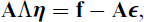
or, in terms of covariances, as

This shows Var(η) can be obtained from Var(
Note that Croon (2002) derived this formula in scalar form for each of the elements of the factor covariance matrix Var(η), and, moreover, assumed the measurement models were estimated separately for each factor involved. The more general form given here allows for the simultaneous estimation of the measurement models of all factors, which is required when there are cross-loadings or correlated residuals among items loading on different factors (Hayes and Usami, 2020). As can be seen, the terms 
Based on this equation, Hoshino and Bentler (2013) proposed equating the diagonal elements of Var(η) to the estimated factor variances from the first step and the off-diagonal elements to the corresponding entries in Var(f). This works because the off-diagonal elements of
Croon’s bias adjustment has been extended for dealing with various types of more complex structural models, such as for micro-macro multilevel analysis (Croon and van Veldhoven, 2007), multilevel path analysis (Devlieger and Rosseel, 2019), and path models with latent interactions (Cox and Kelcey, 2021; Rosseel et al., 2022).
Although the local SAM approach by Rosseel and Loh (2024) is similar to Croon’s approach, it uses a slightly different starting point. In local SAM, we rewrite equation 2.5 as follows
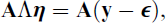
where 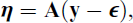
or, in terms of covariances,

The form of
Recently, Perez Alonso et al. (2024) proposed a rather advanced application of the SAM approach; that is, they used it for estimation of a mixture multigroup SEM. Their measurement model consists of a multiple group factor analysis (for many groups) and their structural model uses the group-specific factor covariances in a mixture model aimed at clustering the groups based on their structural parameters.
Similar to Croon’s method and local SAM, Gerbing and Anderson (1987) and Lance et al. (1988) proposed estimating the structural parameters using Var(η) as data matrix. However, rather than using bias-adjusted factor scores or a mapping matrix, they used the fact Var(η) equals the step-one factor covariance matrix Φ when the measurement models for all latent variables appearing in the structural model are estimated as a single block with an unrestricted factor covariance matrix.
Background
When the latent variables are continuous and the observed variables are ordinal categorical, the measurement model may take on the form of a categorical factor analysis (CatFA). As factor analysis with continuous observed variables, CatFA involves estimating a linear factor model, but with the observed variables’ polychoric correlation matrix instead of their covariance matrix as input data (see, e.g., Forero et al., 2009). Parameters are typically estimated by diagonally weighted least squares (DWLS; Christoffersson, 1977; Muthén et al., 1997).
With continuous latent variables and categorical observed variables, the measurement model may also be a latent trait or IRT model (Bartholomew and Knott, 1999; van der Linden, 2017), typically estimated using marginal maximum likelihood. A unidimensional latent trait model for response pattern 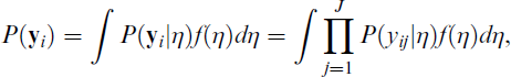
where the probability of the response of person i on item j conditional on the latent trait value η, 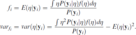
Since there is no closed form expression for the integral, it has to be solved either numerically or by Monte Carlo simulation.
Fixed parameters
One particular fixed parameters approach for dealing with continuous latent variables and categorical observed variables is the global SAM approach. Although not mentioned explicitly by Rosseel and Loh (2024), their global SAM approach can also be applied in combination with a CatFA for dichotomous or ordinal items. This method is implemented in the lavaan package in R.
Kuha and Bakk (2023) proposed a two-step approach which involves fixing the latent trait measurement parameters defining the conditional response probabilities
The MUPPET approach for factor analytic models has recently been extended to allow for latent trait type measurement models (Levy and Neish, 2024). MUPPET uses a two-stage Bayesian estimation method for dealing with covariates and outcome variables.
Single indicator
Lai and Hsiao (2022) showed how the single-indicator approach they refer to as two-stage path analysis can be used with latent variable scores obtained from a latent trait model. They proposed using EAP trait scores, which are IRT based equivalents of regression factor scores. Related work was done by Wang et al. (2019), who applied the single-indicator approach to deal with measurement error in MAP latent trait scores used as the outcome variable in a linear mixed effects model.
As explained above for the continuous indicators case, with regression (and thus EAP) factor scores we can fix the loadings of the factor scores to their reliability ρ and their residual variance to φρ(1 − ρ). However, different from the factor analytic case, the reliability of IRT-based trait scores varies across individuals because the EAP scores’ posterior variance, 
and
as fixed loading and residual variance for person i. Note that, similar to the factor analysis case, φ can be obtained from the individual factor scores and their variances; that is, by using
Note that the single-indicator approach using latent trait scores would be much simpler and, moreover, computationally less demanding if we replace
Although not described in the Rosseel and Loh (2024) paper, their local SAM approach is available in the lavaan package for categorical variables. First CatFA models are estimated using DWLS and subsequently equation 2.10 is applied with a Barlett mapping matrix and Var(
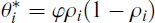
Although not proposed in the literature yet, it also seems possible to implement Croon’s approach with EAP trait scores from IRT measurement models. We saw that with regression factor scores 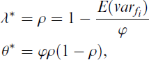
with
While such an adjustment does not account for the heterogeneous measurement error, it is also possible to apply the correction with individual-specific 
and for a covariance between two factors η1 and η2

Hoshino and Bentler (2013) indicated their stepwise procedure using maximum likelihood factor scores can also be applied with IRT type measurement models. As was explained above for factor analytic models, their approach involves equating the diagonal elements of Var(η) to the estimated true factor variances from the first step and the off-diagonal elements to the factor score covariances.
Categorical latent variables
Background
Denoting the single discrete latent variable by η, a particular class by c, and the number of classes by C, a latent class measurement model for P(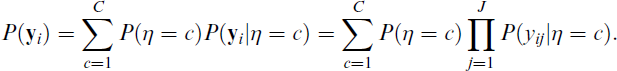
Here
The above formula is the one for a simple latent class measurement model. The most common extension containing a structural part involves including covariates 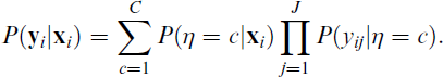
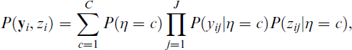
Other common extensions containing a structural part are models with a distal outcome zi affected by class membership,
as well as models with multiple latent variables affecting each other, for example, η1 affecting η2,

The structural parameters of interest are the regression coefficients defining
Latent class predictions fi based on the latent class measurement model can be obtained based on the posterior membership probabilities 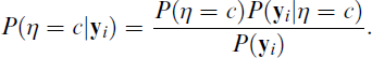
The standard practice is to assign individuals to the class with the largest posterior probability, which yields MAP estimates. Other options are random assignment or proportional assignment (Bolck et al., 2004). As shown by Bolck et al. (2004), the assignment method used defines the values of
Fixed parameters
Bakk and Kuha (2018) proposed a two-step latent class analysis approach, which involves fixing latent class measurement parameters defining the conditional response probabilities
Applications of the fixed parameters approach with more complex structural models concern the three-step latent Markov model by Bartolucci et al. (2015) and the two-step multilevel latent class model by Di Mari et al. (2023). In both applications, the first step involves estimating the measurement model parameters, while ignoring the (longitudinal or multilevel) dependence structure in the data.
Although not yet mentioned in the literature, the fixed measurement parameters approach can be used without any modification with continuous response variables, that is, with latent profile and other types of mixture models. In that case, the fixed parameters in the estimation of the structural model of interest are the class-specific means and (co)variances defining the multivariate densities
Single indicator
For latent class models with covariates, Bolck et al. (2004) derived the relationship between 
As noted by Vermunt (2010), this is the equation of a latent class model with covariates 
Vermunt (2010) proposed a slight modification of this formula, which involves replacing P(
Important advantages of this modification are: (a) it prevents the possibility of summing over a very large numbers of data patterns; (b) as shown by Gudicha and Vermunt (2013), it also works with latent profile and other mixture models for continuous observed variables, where the summation over all possible
As shown by Bakk et al. (2013), the three-step ML approach can not only be used for latent class models with covariates, but also for latent class models with a distal outcome and SEM-like models with multiple discrete latent variables. Moreover, this stepwise modelling approach has been used with latent Markov models (Di Mari et al., 2016; Vogelsmeier et al., 2023a), multilevel latent class models (Lyrvall et al., 2024), latent class tree models (van den Bergh and Vermunt, 2019), and inverse propensity weighting for the estimation of the causal effect of a treatment on latent class membership (Clouth et al., 2022, 2023).
A similar stepwise approach for investigating the relationship between class membership and a distal outcome zi was proposed by Lanza et al. (2013). They proposed including zi as covariate in the step-one latent class model, which gives posterior class membership probabilities containing information on its association with the latent classes. For the structural model estimation, they use in fact a single-indicator approach with proportional class assignment, but without the need to correct classification errors.
The BCH method (Bolck et al., 2004) is a bias adjustment approach for latent class and latent profile models. Similar to the single-indicator approach, it is based on equation 4.1 which shows the relationship between
As shown by Vermunt (2010), the BCH approach can be conceptualized as an analysis of an expanded dataset with C records per person with weight wic. Denoting the elements of 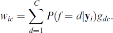
Note that the class assignment probabilities
The three-step BCH approach can also be used with distal outcome models (Bakk et al., 2013). In fact, it has been shown to be superior to the three-step ML approach when the outcome variable is a continuous variable (Bakk and Vermunt, 2016). Bolck et al. (2004) and Bakk et al. (2013) showed how to apply this approach with multiple latent variables. Lê et al. (2025) proposed using the BCH approach together with inverse propensity weighting for the estimation of the causal effect of latent class membership on an outcome variable.
Remaining topics
In this section, we discuss various remaining topics which are relevant for the practical application of stepwise latent variable modelling approaches. These include heterogeneous measurement or classification error resulting from measurement non-invariance and missing data on the latent variable indicators, correcting standard error estimates for the stepwise modelling, and software implementing stepwise modelling approaches.
Heterogeneous measurement or classification error
When discussing the implementation of the single-indicator approach with IRT type measurement models (Lai and Hsiao, 2022), we already touched upon the topic of heterogeneous measurement error. Our tentative conclusion was that ignoring the heterogeneous nature of the measurement errors probably has little impact on the structural parameter estimates as long as it is uncorrelated with the other variables appearing in the structural model.
Another situation in which measurement or classification errors are heterogeneous occurs when there is missing data on the response variables
Heterogeneous measurement and classification errors also occurs when the step-one model accounts for measurement non-invariance or differential item functioning (van der Linden, 2017). In that case, the terms λ∗ and Θ∗ or the
It should be noted that whether to account for or to ignore heterogeneous measurement or classification error is not an issue in the fixed parameters approach, since it does not involve estimation of the latent variables scores as an intermediate step. Instead, one fixes the measurement parameters, which may differ per group if one accounted for measurement non-invariance in the first step.
Standard error computation
In the fixed parameters and the single-indicator approach, we treat either the estimated parameters from the measurement model or functions of these as known when estimating the structural model parameters. As shown by Oberski and Satorra (2013) and Rosseel and Loh (2024) for the continuous latent variable case and by Bakk et al. (2014) and Bakk and Kuha (2019) for the discrete latent variable case, standard errors can be corrected for the fact that these are in fact estimates with their own sampling variation when the structural parameters are estimated by maximizing a log likelihood, which known as pseudo-maximum likelihood estimation (Gong and Samaniego, 1981).
Let Σ
S
contain the uncorrected covariances of the parameters of the structural model, Σ
M
the covariances of the measurement parameters or, in the single-indicator case, of functions of these, 
In the single-indicator approach ΣM can be obtained from the covariances of the measurement parameters using the delta method. Bakk et al. (2014) illustrated this for the latent class analysis case; that is, for the three-step ML procedure in which ΣM contains the covariances of the log
Similar types of standard error corrections are not available for the bias adjustment approach. This is why, for example, the lavaan package reports global SAM based standard errors when using the local SAM procedure. However, when applying the BCH approach for discrete latent variables, one should account for the fact that the expanded dataset contains multiple records per person and, moreover, BCH weights. As proposed by Vermunt (2010), this can be dealt with using complex sampling (or cluster-robust) standard errors. Robust standard errors were also proposed by Bartolucci et al. (2015) for their three-step latent Markov approach.
As an alternative to the frequentist approach of fixing measurement model parameters to their first-stage point estimates and subsequently adjusting the standard error estimates, one may use Bayesian multiple-stage MCMC estimation, as done in MUPPET modelling. This involves dealing with parameter uncertainty by accounting for the full first-stage posterior parameter distribution when estimating the structural parameters (Levy, 2023; Levy and McNeish, 2024). Similar Bayesian estimation methods could be developed for single indicator and bias adjustment approaches. For example, in the single-indicator approach, instead of using a single set of latent variable scores obtained with point estimates of the measurement parameters, one could use multiple sets of latent variable scores drawn from their posterior distribution while accounting for the uncertainty of the measurement parameters.
Software implementations
Most of the stepwise approaches we discussed are available in latent variable modelling software. However, with some additional some effort, each of the approaches can be implemented without specific stepwise modelling routines. The fixed measurement and single-indicator approaches can be implemented in SEM or latent class analysis software that allows imposing fixed value constraints on the model parameters. Slightly more tedious to implement is the heterogeneous measurement case resulting from an IRT type measurement model, for which Lai and Hsiao (2022) provided example code for OpenMx (Neale et al., 2016). The bias adjustment approach for continuous latent variables involves creating an adjusted factor covariance matrix, which can subsequently be used as input data for any structural modelling software. For categorical latent variables, one should create an expanded dataset containing the BCH weights, after which any type of structural model can be estimated using a weighted analysis. The only requirement is that the routine used to estimate the structural model accepts negative weights.
LatentGOLD (Vermunt and Magidson, 2016, 2025) is one of the programs that contains options for stepwise latent variable modelling. For latent class models, it implements each of the three approaches, which it refers to as the Bakk-Kuha, ML, and BCH adjustment methods. In version 6.1, it also implements the single-indicator approach for continuous latent variables, where the step-one model can be either a factor analysis or latent trait analysis. After estimation of the measurement model of interest, one saves the posterior probabilities or the logdensities of the latent class model, or the EAP factor scores and their standard errors from the factor analytic or IRT model to an output data file. This information suffices to set up the structural model, where it is possible to indicate that the measurement or classification errors are heterogeneous across levels of a grouping variable. For latent class models, the most common types of structural models (including latent Markov models) are available via the Step3 point-and-click module. Other stepwise latent class models, such as path models for multiple discrete latent variables and multilevel latent class models, can be specified via the syntax system. The structural model for continuous latent variables should always be specified with LatentGOLD’s syntax system, where not only a simple regression or path model can be specified, but also a more complex model, such as a mixture multiple group SEM (Perez Alonso et al., 2024) or a dynamic factor model (Rein et al., 2025).
Mplus (Asparouhov and Muthén, 2014) implements the ML (single indicator) and BCH (bias adjustment) approaches for latent class models in an automated form for simple structural models (covariates and distal outcomes). However, it also allows saving BCH weights to an output file and using these weights in subsequent analysis for the estimation of more complex structural models with latent classes. The BCH approach is also available as SAS (SAS Institute Inc., 2010) and Stata (Statacorp, 2025) functions for dealing with covariates and distal outcomes (Dziak et al., 2017, 2022).
R packages (R Core Team, 2024) implementing stepwise latent variable models include lavaan (Rosseel, 2012), multilevLCA (Lyrvall et al., 2023), lmfa (Vogelsmeier et al., 2023b) and tidySEM (van Lissa, 2019). Lavaan implements the fixed parameters and bias adjustment approaches for factor analysis and CatFA measurement models, and refers to these as global and local SAM. The multilevLCA package implements standard and multilevel latent class analysis with covariates for binary response variables estimated using a two-step (or fixed parameters) approach. The lmfa package implements the single-indicator approach for a continuous-time latent Markov model with covariates for intensive longitudinal data, where the first step is a mixture factor analysis. Finally, tidySEM contains a BCH function for estimating structural models in which the latent classes are treated as the grouping variable.
In addition to full R packages, various recent publications include R code which allows researchers to apply the newly proposed method concerned with their own data. Examples include two-step path modelling (Lai and Hsiao, 2022), MUPPET (Levy, 2023; Levy and McNeish, 2024), mixture multiple-group SEM (Perez Alonso et al., 2024) and stepwise latent vector autoregressive modelling (Rein et al., 2025).
Discussion
An overview of stepwise latent variable approaches was provided. It was shown that similar approaches have been proposed for factor analytic, latent trait, and latent class type measurement models. These involve using fixed measurement parameters, latent variable predictions as single indicators, or Croon’s or similar bias adjustments of the latent variable predictions. We explained the logic underlying these approaches with the appropriate references, as well as references to applications in combination with more complex structural models. Moreover, we explained how Croon’s method can also be implemented with IRT-based measurement models.
Special attention was paid to the issue of heterogeneous measurement and classification errors, which occurs with IRT models, with missing values on the latent variable indicators, and with measurement non-invariance. When a grouping variable causing the measurement invariance is also used in the structural model, the heterogeneity should clearly be taken into account. In most other situations, it appears that the heterogeneity can be ignored, but this is something that needs further investigation.
We showed how to obtain standard errors corrected for the stepwise estimation. However, it has also been reported that this correction is not needed or that it may even yield too conservative tests if the measurement or classification errors are not large, and the sample is not small. This issue is also a topic requiring further investigation. Moreover, work remains to be done for the bias adjustment approaches for which standard error correction is not yet available. Interesting is the Bayesian MUPPET modelling approach, which accounts for the stepwise estimation in a rather straightforward manner. Similar Bayesian estimation methods may be developed for application in conjunction with single indicator or bias adjustment approaches. Another popular approach for improved standard error estimation in stepwise modelling is bootstrapping, which surprisingly has not yet been investigated in the context of stepwise latent variable modelling.
We discussed software implementations of the stepwise approach, which include LatentGOLD, Mplus, packages and code written for R, as well as functions written for Stata and SAS. Given that this is a lively field of research, surely, more software for stepwise latent variable modelling will become available in the near future. An important application of the stepwise estimation methods discussed in this article is in big data analytics. Significant computational efficiency gains can be achieved using these stepwise approaches, provided the available software is capable of handling very large datasets.
Footnotes
Declaration of Conflicting Interests
Jeroen Vermunt is a co-developer (along with Jay Magidson) of the LatentGOLD software. While LatentGOLD is a commercial program, as of January 2025, it is free for academic use.
Funding
The authors received no financial support for the research, authorship and/or publication of this article.