
Abstract
Mixture of factor analysers (MFA) are popular tools for dimension reduction and model-based clustering. The conventional method of parameter estimation for MFA is via maximum likelihood using the Expectation-Maximization (EM) algorithm. This typically assumes the number of components (g) and the number of factors (q) to be known a priori, which are often not known in practice. This article reviews different approaches for automatically inferring g and/or q from the data. A hybrid method, incremental automated MFA (IAMFA), is also proposed. We conduct a systematic comparison of these methods using simulated data and analyse their relative performance across various scenarios, looking at their ability to infer g and q correctly, the general model fit, clustering accuracy, and computation time.
Introduction
Mixtures of factor analysers (MFA) are frequently used for modelling high dimensional data with heterogeneous structure. The MFA model combines a mixture model with the factor analysis (FA) model, thus able to perform both clustering and dimension reduction at the same time. Initially introduced by Ghahramani and Hinton (1997), the method had since found many applications in a wide range of areas, from microarray gene expressions (McLachlan et al., 2003), image processing (Yang et al., 1999), to financial risk modelling (Ko and Beak, 2018).
Parameter estimation of the MFA model is typically carried out using the maximum likelihood estimation method via the Expectation-Maximization (EM) algorithm (Dempster et al., 1977). Several EM-type algorithm have been proposed for the MFA model, including the Expectation Conditional Maximization (ECM) algorithms by Ghahramani and Hinton (1997), McLachlan and Peel (2000a) and Zhao and Yu (2008). These algorithms typically assume the number of components (g) and the number of factors (q) to be known in advance. However, in practice, g and q are often unknown and need to inferred from the data. To this end, there have been a number of attempts to determine g and/or q in an automated manner. Many authors perform an exhaustive search by fitting (one or more) MFA models for different values of g and q and then selecting a suitable model based on some information criteria. A main drawback of this approach is the high computation time. Kaya and Salah (2015) proposed an adaptive MFA algorithm which infers both p and q by progressively splitting a component/factor and then incrementally merging components. Wang and Lin (2020) proposed an automated MFA algorithm where q is estimated during the execution of an EM algorithm, but assumes g to be known in advance. On the other hand, several others have considered Bayesian inference, including the variational Bayesian MFA (Ghahramani and Beal, 1999), the infinite mixtures of infinite FA (Murphy et al., 2020), the overfitted mixtures of infinite FA (Murphy et al., 2020) and more recently, the dynamic mixture of MFA (Grushanina and Frühwirth-Schnatter, 2023).
This article presents a systematic comparison of automated approaches for determining g and/or q (and the remaining parameters) of the MFA model. Note that we do not aim to provide a comprehensive survey of all existing methods, but rather focus on those where there are publicly available software implementations. In addition, we propose a new method for inferring g and q—the incremental automated MFA (IAMFA) algorithm—where g is determined in an incremental manner and q is inferred based on an approximated information criterion. Performance of the methods was evaluated on 100 replications of each of 12 different scenarios. We assessed their performance based on the accuracy of the inferred value of g and q, the time taken to run the algorithm, the quality of the fitted models, and the correctness of cluster assignments.
The remainder of this article is organized as follows. In Section 2, we briefly review the MFA model and a commonly-used ECM algorithm to fit the model. In Section 3, we examine selected methods for inferring g and/or q. We also propose the IAMFA algorithm. An implementation of these methods are available from the R (R Core Team, 2025) packages
The mixture of factor analysers (MFA)
The mixture of factor analysers (MFA) is a mixture model where each component of the mixture follows the well-known factor (FA) analysis model. The latter postulates that the p-dimensional data vector
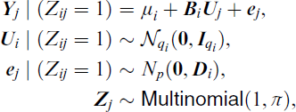
for i = 1, 2, …, g and j = 1, 2, …, n, and where
It follows that the MFA model can be formulated as a Gaussian mixture model (GMM) with a ‘restricted’ component covariance matrix,
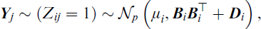
with density given by

where
It is well-known that the MFA model suffers from identifiability issues. To ensure the number of parameters in the MFA model is less than that of a GMM model with a full component covariance matrix, the number of factors for each component (qi) of the MFA model is required to obey the Ledermann bound (Ledermann, 1937), given by

for i = 1, 2, …, g. Apart from this, the MFA model inherits from the FA model the property of invariance to orthogonal transformations. This means post-multiplying a factor loading matrix
In addition, it is often assumed that the number of factors for each component of the MFA model is the same, that is, qi = q for all i. This assumption is made in most of the methods considered in Section 3. Another popular assumption is to have a common error-variance matrix across all components, that is,
For a fixed g and q, the parameters of the MFA model Ω can be estimated using an EM algorithm and generalizations thereof, such as the ECM algorithm (Meng and Rubin, 1993), the Alternating Expectation Conditional Maximization (AECM) algorithm (Meng and van Dyk, 1997), or the Parameter Expanded Expectation Maximization (PX-EM) algorithm (Liu et al., 1998). For example, Ghahramani and Hinton (1997) described an ECM algorithm for the MFA model, treating the factors
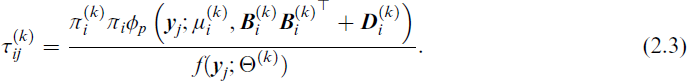
The M-step then updates the parameters in Θ using

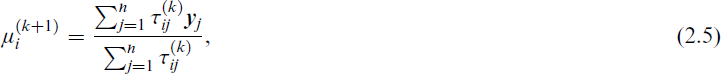

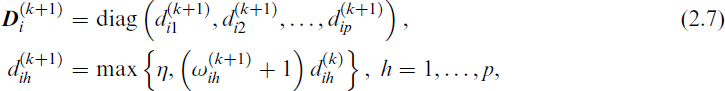
where
We now consider algorithms in the literature that can infer g, q, or both g and q. In addition, we describe a new algorithm denoted by IAMFA in Section 3.7. The majority of these algorithms are based on either the ECM algorithm by Ghahramani and Hinton (1997) or the alternative version by Zhao and Yu (2008). Many of these algorithms attempt to choose g using a hierarchical splitting approach, that is, by starting with a single component model and then gradually splitting into more sub-components based on certain criteria. There are a number of different approaches proposed for choosing q. Some methods choose q based on an approximation of the Bayesian information criterion (BIC) (Schwarz, 1978), defined as −2 log(likelihood) + m log n, where m is the number of parameters in the model. Another attempts to choose q by comparing the sample covariance structure with the modelled covariance structure of each component of the MFA model and then adds an extra factor to the component with the largest difference between these two structures. There are also a few attempts based on the Bayesian formulation of the MFA model, typically employing a non-parametric prior for g and/or q to achieve automatic inference. They usually allow for each qi to be different.
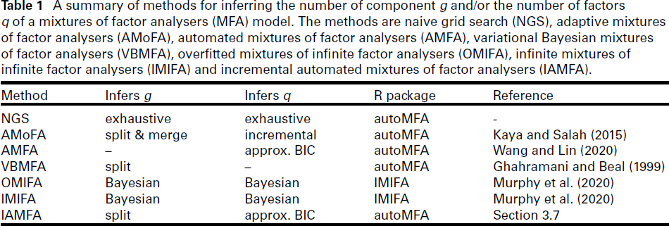
A summary of methods for inferring the number of component g and/or the number of factors q of a mixtures of factor analysers (MFA) model. The methods are naive grid search (NGS), adaptive mixtures of factor analysers (AMoFA), automated mixtures of factor analysers (AMFA), variational Bayesian mixtures of factor analysers (VBMFA), overfitted mixtures of infinite factor analysers (OMIFA), infinite mixtures of infinite factor analysers (IMIFA) and incremental automated mixtures of factor analysers (IAMFA).
A summary of methods for inferring the number of component g and/or the number of factors q of a mixtures of factor analysers (MFA) model. The methods are naive grid search (NGS), adaptive mixtures of factor analysers (AMoFA), automated mixtures of factor analysers (AMFA), variational Bayesian mixtures of factor analysers (VBMFA), overfitted mixtures of infinite factor analysers (OMIFA), infinite mixtures of infinite factor analysers (IMIFA) and incremental automated mixtures of factor analysers (IAMFA).
In the subsections to follow, we provide an overview of several existing methods for inferring the number of components and/or factors in MFA models, along with our proposed IAMFA algorithm. The methods considered are naive grid search (NGS), adaptive mixtures of factor analysers (AMoFA), automated mixtures of factor analysers (AMFA), variational Bayesian mixtures of factor analysers (VBMFA), overfitted mixtures of infinite factor analysers (OMIFA) and infinite mixtures of infinite factor analysers (IMIFA). A summary of these methods is presented in Table 1, with further details provided later in the section.
The most intuitive and simplest method for automatically choosing g and q is perhaps performing an exhaustive search over different combinations of g and q. This method, which we call naive grid search (NGS), serves as a baseline for systematically evaluating all possible combinations of g and q within predefined ranges.
Given a range of plausible values for g and q (i.e., 
evaluations of the ECM algorithm. Even with small values of ns, gmax and qmax (such as ns = 10, gmax = 10 and qmax = 5), NGS would need a large number of ECM evaluations (500 in this example). For small datasets where the execution of the ECM algorithm is very fast, this approach may be reasonable. However, the computational cost can become prohibitively high for large datasets, rendering it infeasible in practice.
Adaptive mixtures of factor analysers (AMoFA)
Kaya and Salah (2015) introduces a dynamic model selection approach based on the minimum message length (MML) criterion (Wallace and Boulton, 1968). Rather than searching over all possible candidate models as in NGS, AMoFA iteratively splits existing components or merges them to optimize the trade-off between model complexity and fit. The MML criterion functions similarly to BIC, but includes additional complexity penalty to discourage complex models. By incrementally increasing model complexity only when justified by the data, the AMoFA approach avoids unnecessary computations while still ensuring a reasonable fit.
The algorithm comprises two phrases: an incremental phrase and a decremental phrase. It begins by fitting a single component single factor MFA model to the data (i.e., (g, q) = (1, 1)) using a slightly modified version of the ECM algorithm by Ghahramani and Hinton (1997). During the incremental phrase, AMoFA progressively splits a mixture component into two or adds a new factor to an existing component until the decrease in MML is less than a specified threshold. It then enters the decremental phrase, where components are progressively merged until only one component remains. The final model is chosen to be the model with the lowest MML value found throughout the entire process. A summary of the AMoFA algorithm is presented in Algorithm 1 in Appendix B. For technical details of the splitting and merging process, the reader is referred to Kaya and Salah (2015). It should be noted that the AMoFA allows each component to have its own number of factors qi.
Automated mixtures of factor analysers (AMFA)
More recently, Wang and Lin (2020) proposed the automated mixtures of factor analysers (AMFA) algorithm that can estimate q without an exhaustive search or splitting/merging. AMFA modifies the EM algorithm by treating q as a parameter to be estimated rather than fixed a priori. It uses an approximation of the BIC to determine q, effectively embedding a regularization mechanism into the model-fitting process. The AMFA approach is a generalization of the automated factor analysis (AFA) algorithm by Zhao and Shi (2014) and is based on the ECM algorithm by Zhao and Yu (2008). With this approach, the value of q is estimated by minimizing the following approximation of the BIC,

where
A number of attempts have been made to infer g and q using Bayesian techniques. One of the earlier attempts is Ghahramani and Beal (1999), who proposed the variational Bayesian mixture of factor analysers (VBMFA) based on a Bayesian formulation of the MFA model. The method makes use of the variational Bayesian expectation-maximization (VBEM) algorithm. We will not provide a full description of the VBMFA algorithm (see Beal (2003) for details), but instead focus on the inference process of g and q.
The inference of the number of components g is performed through an incremental process. It begins by assuming a single component and then progressively introduces new components through a mechanism known as component birth. At each step, a new component is added and the model is re-evaluated to check whether this addition improves the model fit. If no improvement is achieved, or if the specified maximum number of attempts have been reached, the process terminates. This allows the model to determine the most appropriate number of components while balancing model complexity and fit to the data.
The inference of q is handled using automated relevance detection (ARD) priors. ARD allows the model to automatically decide which factors (i.e., which columns of the factor loading matrices
Despite the elegance of VBMFA in theory, practical implementation can present challenges. For instance, in our testing (using both our R implementation in
Overfitted mixtures of infinite factor analysers (OMIFA)
OMIFA (Murphy et al., 2020) takes a non-parametric Bayesian approach by initializing with an over-specified number of components and factors and then gradually eliminating unnecessary components or factors based on data, guided by posterior probabilities. As the name suggests, it is a generalization of the infinite factor analysers (Bhattacharya and Dunson, 2011) to the mixture setting. It adopts an over-fitting finite mixture strategy. The model is initialized with a deliberately large number of components
For the factor-analytic part, OMIFA employs the multiplicative gamma process (MGP) shrinkage prior on each factor loading matrices
Infinite mixtures of infinite factor analysers (IMIFA)
In the same article, Murphy et al. (2020) generalized OMIFA to IMIFA by embedding the factor analysis model into an infinite mixture framework. The primary distinction of IMIFA from OMIFA is the use of the Pitman-Yor process (PYP) for modelling the mixing proportions, replacing the fixed-g overfitting strategy used in OMIFA. The PYP generalizes the Dirichlet process, allowing heavier-tailed cluster-size distributions and hence richer partition structures. As in OMIFA, IMIFA uses the MGP prior to infer the number of factors. The MGP enables the model to adaptively determine the number of active factors, pruning irrelevant ones by assigning smaller or zero loadings to unimportant factors. This combination of a PYP prior for g and MGP shrinkage for qi gives IMIFA great flexibility in adapting both the number of clusters and the dimension of each factor subspace.
Together, OMIFA and IMIFA share the same infinite-factor mechanism but differ in how they handle the component count: OMIFA prunes an over-specified finite mixture, whereas IMIFA learns g from a non-parametric prior.
Incremental automated mixtures of factor analysers (IAMFA)
We now introduce a hybrid algorithm that combines the strengths of AMFA and AMoFA, called the incremental automated mixtures of factor analysers (IAMFA) model. It infers g and q automatically using a progressive model-building approach. Specifically, q is inferred using the approximated BIC approach in AMFA and g is determined using an incremental approach similar to AMoFA and VBMFA. These modifications allow IAMFA to efficiently infer g and q while maintaining computational feasibility.
The algorithm begins with the simplest model—a single-component single-factor MFA model—fitted using the ECM algorithm described in Section 2. It then adopts a component-splitting strategy similar to AMoFA, but uses BIC in place of MML for model selection. This choice is motivated by the common use of BIC in penalized likelihood methods. Furthermore, empirical testing indicated that BIC achieves comparable model selection performance to MML while being computationally more efficient. Initially, the single component model will be split into a two-component model. Allocation of data points to the new component is determined in the same way as the assignment of points to the ‘child’ components in VBMFA (see Appendix H and also Beal (2003) for technical details). Parameter estimation of the two-component model is carried out via the AMFA algorithm given in Algorithm 2. Note that the number of factors q is updated during the execution of Algorithm 2. If the split results in a higher BIC value, the attempt is discarded and a new split is attempted. If no improvements to the BIC is made after a specified number of attempts, then the fitting process is terminated. Otherwise, the first split that decreases the BIC is accepted.
Then, the splitting process is repeated, but now involves a multivariate kurtosis metric. The kurtosis is chosen as it effectively captures deviations from normality that suggest a mixture component may contain multiple sub-clusters. While skewness measures asymmetry and number of modes detects multimodality, kurtosis is a more stable indicator of potential misspecified component structure. This aligns with prior findings (Beal, 2003) and empirical experiments in our study. Specifically, the splitting will be attempted in order of decreasing multivariate kurtosis metric 
and where
It should be noted that all proposed splits—whether the initial or subsequent—are accepted only if they result in a lower BIC value. The multivariate kurtosis metric is used solely to rank the components in order of priority for splitting: at each iteration, the component with the highest kurtosis is selected first. If no split yields an improved BIC after a specified number of attempts, the algorithm terminates. A summary of the IAMFA algorithm is presented in Algorithm 3, in Appendix D. We implemented this algorithm in the R package
A systematic simulation study is carried out to compare the performance of the methods discussed in Section 3. We use the implementations of these methods that are available from the R packages the dimension of the data (p): low (p = 3) or high (p = 10); the number of factors (q): low the number of components (g): low (g = 3) or high (g = 10); the degree of separation of the components: low or high; the total number of data points in the dataset (n): low (n = 60g) or high (n = 240g); whether the dataset is balanced: yes (πi = n/g) or no.
Each dataset in the simulation study is generated from

where
The component means μi are set as follows. We first define the temporary means 
Finally, when p = g = 10, we take
The covariance matrix
For imbalanced dataset, the number of points for each component ni is set as follows. First, each component is initially assigned 30 points. This is to avoid having very small components. The remaining n 30g points are allocated so that the largest component is 10 times larger than the smallest component, with intermediate components obtaining a linearly interpolated fraction of this amount. In effect, we have 
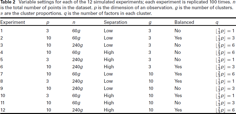
With six variables for the setting and two choices for each variable, there will be 26 = 64 different combinations of the variables. Making use of a 26−2 fractional factorial design by Box (2005), the number of experiments needed can be reduced to 16, at the cost of introducing confounding effects from third and sixth order interactions. Furthermore, four of these combinations (where p = 3 and q = 2) do not satisfy the Ledermann bound (2.2) and hence are discarded. The settings for the remaining 12 experiments are summarised in Table 2. For each setting, we make 100 simulated replications. Hence there is a total of 1,200 simulations.
Variable settings for each of the 12 simulated experiments; each experiment is replicated 100 times. n is the total number of points in the dataset. p is the dimension of an observation. g is the number of clusters. π are the cluster proportions. q is the number of factors in each cluster.
Variable settings for each of the 12 simulated experiments; each experiment is replicated 100 times. n is the total number of points in the dataset. p is the dimension of an observation. g is the number of clusters. π are the cluster proportions. q is the number of factors in each cluster.
The performance of the seven methods is evaluated in five aspects: (a) the computation time, (b) the quality of the model fit according to the BIC, (c) the clustering accuracy according to the adjusted Rand index (ARI) (Hubert and Arabie, 1985), (d) the inferred g and (e) the inferred q. The results are presented in Tables 3 to 5, respectively. In addition, histograms for the inferred values of g and q are given in Figures 1 and 2.
We will give a few general remarks before discussing each of the five aspects. Of the methods considered (and apart from NGS), the AMFA method performed the best, on average, for all of the metrics except the computation time and for inferring q to within an error of ± 2. This is followed by the OMIFA and IMIFA methods which generally performed comparably well. The IAMFA generally performed well, but not as well as the aforementioned methods. Lastly, the AMoFA and VBMFA are almost always the worst performing methods in these experiments.
Additionally, we conducted experiments with a higher dimension of p = 20, as suggested by a reviewer. The same variable settings were used in the p = 10 experiments (i.e., experiments 2, 3, 4, 6, 7, 9, 11, and 12). The observed trends remained consistent with those for p = 3 and p = 10, with the only notable difference being the expected increase in computation time. As these results do not provide new insights, they are not discussed here. However, a summary of computation times is included in Table 11 in Appendix F.
Computation time
The simulation study was performed in R on a mid-range quad-core computer. All experiments were conducted on the same machine and all methods were run under the same computational conditions. We implemented the methods NGS, AMoFA, AMFA, VBMFA, and IMIFA in the R package
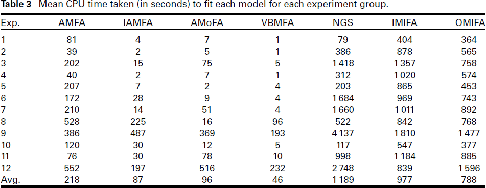
Mean CPU time taken (in seconds) to fit each model for each experiment group.
Mean CPU time taken (in seconds) to fit each model for each experiment group.
The mean CPU time (in seconds) for each method and each experiment is presented in Table 3. On average across all 1 200 trials, VBMFA is the fastest method and (as expected) NGS is the slowest method. Ignoring the NGS method, the difference in mean computation time between the fastest and the (second) slowest is pronounced: VBMFA is almost 34 times faster than IMIFA. The average computation time of the IAMFA and the AMoFA methods are roughly twice that of the VBMFA method, placing them in the second and third place, respectively.
It can be observed from Table 3 that the dimension of the data had a clear impact on the computation time for the NGS method. This is likely because the method is only impacted by the higher computational burden of performing the necessary matrix computations in higher dimensions (as are all of the other models), but it also has to evaluate six times more models, since when p = 10, the Ledermann bound affords qmax = 6 compared to qmax = 1 when p = 3.
Unsurprisingly, the AMFA and NGS methods are generally slower than the VBMFA, AMoFA and IAMFA methods as the last three methods do not involve any exhaustive search. We might expect the AMFA method to be generally faster than the NGS method since the former does not need to search over a range of values for q. However, this was not always the case. For example, in Experiments 1, 5, 8 and 10, NGS was faster than AMFA. We note that in these experiments qmax = 1 (as p = 3) and so NGS only search over g like AMFA. The slight time differences may be due to the implementations of these methods.
Apart from NGS, the IMIFA and OMIFA methods were (on average) the slowest among the methods considered. However, we note that their computation times were considerably less variable than the other methods. This can be observed from the ratio of the longest mean computation time to the shortest mean computation time. For NGS, this ratio is 52.17, whereas for IMIFA and OMIFA it is 4.55 and 4.38 respectively.
Mean BIC for each model and each experiment group. *For IMIFA and OMIFA, the mean BICM is provided.
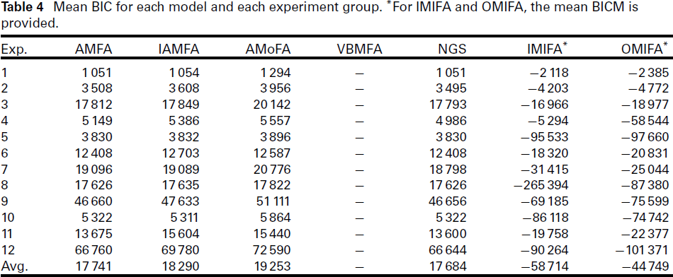
The mean BIC score for each method and each experiment is presented in Table 4. It should be noted that we cannot directly compare the IMIFA and OMIFA methods with the rest of the methods, as the former provided the BIC Monte Carlo (BICM) (Raftery et al., 2007) instead of BIC. As expected, the NGS achieved the lowest mean BIC across all 1 200 simulations. The difference in mean BIC between NGS and AMFA (the second best performing method) is over 50, suggesting the NGS method found better models than the other methods, on average. However, even though NGS generally attained lower mean BIC scores than the competing methods, the difference was very minor in some cases. For example, in Experiments 1, 5, 6, 8, 10, the AMFA method was able to achieve the same mean BIC score (up to four decimal places) as the NGS method.
We also observe from Table 4 that the difference in mean BIC between NGS and AMFA for Experiments 2, 3, 4, 7, 11 and 12 is greater than 10, indicating the NGS outperformed AMFA in these situations. We note that these six experiments correspond to the setting with p = 10. This suggests that AMFA’s ability to find the ‘gold standard’ models (fitted by NGS) is declining as p increases.
The AMoFA method performed poorly across all the experiments, with much higher mean BICs than AMFA and NGS. The IAMFA method also generally performed poorly in the comparison to NGS and AMFA, although it fitted better models in Experiment 10.
For the IMIFA and OMIFA methods, the former produced a lower average BICM score, although OMIFA actually obtained lower BICM in 9 out of the 12 experiments. The main reason that the IMIFA method scored better on average was because in group eight, it obtained an average BICM value whose magnitude was roughly three times that of the OMIFA method. Further investigation showed that this was not due to an outlier BICM value which was biasing the average for the IMIFA. Given this, generally, the BICM criterion is suggesting that in most of the experiment groups the OMIFA method produced better models than the IMIFA method, on average.
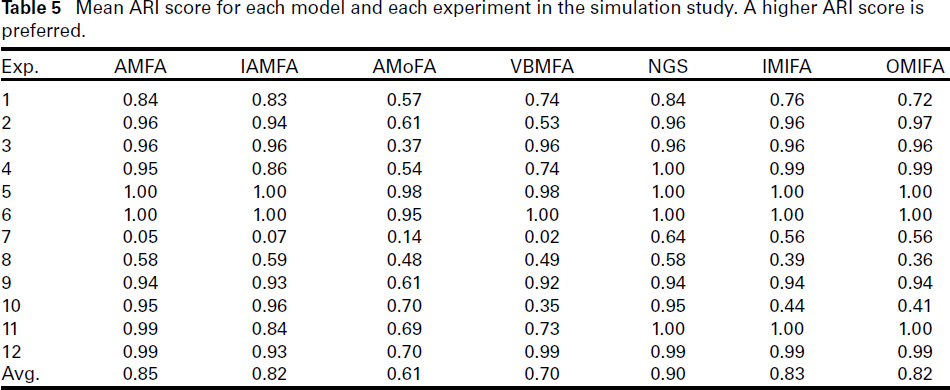
Mean ARI score for each model and each experiment in the simulation study. A higher ARI score is preferred.
Mean ARI score for each model and each experiment in the simulation study. A higher ARI score is preferred.
The mean ARI score for each method and each experiment is presented in Table 5. Note that higher ARI scores are preferred, with the maximum score being one. The NGS method obtained the highest overall mean ARI across all 1,200 simulations. AMFA is the next best performing method, followed by IMIFA, OMIFA, and IAMFA which obtained similar average ARI score. The VBMFA and AMoFA methods performed noticeably worse in terms of average ARI score.
Looking closer at each experiment, we see that NGS always had the highest average ARI score except for Experiment 8 (where IMAFA attained the highest average ARI). The AMoFA method performed worse in the majority of the experiments. Of particular note is that VBMFA behaves erratically. It achieved comparable average ARI score to the NGS method in Experiments 3, 5, 6, 9 and 12. These experiments all have high n, suggesting a possible link between VBMFA’s ability to recreate the underlying sub-population structure and the size of the dataset being used. However, in Experiment 8 (where n is also high), VBMFA performed very poorly and its performance was even worse than some of the experiments where n was low.
Concerning IMIFA and OMIFA, they obtained average ARI scores that are very close to the NGS method in most of the experiments apart from Experiments 1, 7, 8 and 10. Of these, all but Experiment 10 were not well-separated, implying a possible relationship between the separation of clusters and the these two methods’ ability to recreate the sub-population structure of the datasets.
Experiments 7 and 8 were the cases where all methods produced relatively low average ARI scores. There were g = 10 clusters in both cases and the clusters were not well-separated. Several of the clusters could be overlapping, making it challenging for the algorithms to correctly identify all ten components. We observe that all of the methods (except AMoFA) tend to underestimate g in these two experimental settings. In Experiment 7, NGS outperformed the other methods by a large margin. In Experiment 8, IAMFA obtained the highest average ARI score, followed by NGS and AMFA.
Inference on g
To assess how well the different methods inferred g, we calculated two metrics: the proportion of times they correctly obtained the true value of g and the proportion of times they obtained a value that is within 2 of the true value of g. We also fitted a Rasch model (Rasch, 1960) to each of these two cases. The proportion of times where each method inferred g correctly is summarized in Table 6 and the proportion of times each method inferred g correctly within 2 is summarized in Table 10. The ability parameter for each method as given by the Rasch model is listed in Table 7.
Unsurprisingly, NGS achieved the highest overall proportion of times where it inferred g correctly, as well as inferring g to within 2. The second-best performing method in Table 6 is AMFA. This is not surprising, given than AMFA performs a grid search over g. Overall, the worse performing method is AMoFA. The Rasch model ability estimates in Table 7 paint a similar picture. We see that NGS has the highest ability estimates in both metrics (for g and for g ± 2). The AMFA method has the second highest ability estimates.
Looking at each experiment, we see that NGS was able to determine g correctly the majority of times. In fact, it was able to determine the correct g 100% of the time in 7 out of the 12 experiments (Experiments 2 to 6 and 11 and 12).
All of the models tended to perform better, on average, when g = 3 compared to when g = 10. This effect is especially evident in Table 6, where the first six rows correspond to the settings with g = 3. We observed near perfect scores in these rows for all methods except VBMFA. This suggests, in general, the methods may be able to infer g more accurately when the true number of components is small.
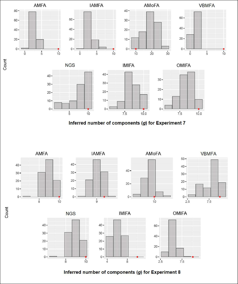
All the methods performed poorly in Experiments 7 and 8. As revealed in Figure 1, the histogram of inferred g by each method shows that almost all methods (apart from AMoFA) tended to underestimate the number of components in these experimental settings. In particular, IMIFA and OMIFA seriously underestimated g in Experiment 8. The AMoFA method, in contrast, overestimated the number of components in Experiment 7.
On examining histograms similar to Figure 1 for the other experiments (not shown), we found that AMFA generally performed similarly to NGS, with the exception of Experiment 7. The AMoFA method generally had the poorest performance amongst the methods considered. It routinely and dramatically overestimated the number of components, sometimes even upwards of 40 components. The VBMFA method tended to underestimate g. The IMAFA method performed relatively well, except in Experiment 7.
Inference on q
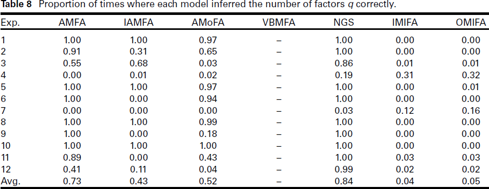
We use the same two metrics in Section 5.4 to assess how well each methods infer the number of factors q. The results are presented in Tables 7, 8, and 9.
Overall, the NGS method inferred q correctly the highest proportion of the time, a result not surprising. AMFA won the second place according to Table 8, with an overall average of 73%. At the other end, IMIFA and OMIFA were the least effective methods, with an overall average of around 4%. Inspection of Table 8 reveals that they incorrectly inferred q for all 100 replications in several experiments. The exception was Experiment 4, where they correctly inferred q about 30% of the time, whereas all the methods were less than 20%. Interestingly, the second metric (where we allow for an error of ±2) paints a very different picture; see Table 9. The IMIFA and OMIFA methods both achieved perfect scores in all experiments. The NGS followed closely behind, with an overall score of 99.67%. The AMoFA and IAMFA methods score poorly on this metric. The results implies that while IMIFA and OMIFA were not able to infer q exactly very often, but they were able to infer values very close to the true q very consistently.
Inferred number of components g for Experiments 7 and 8. The position of the red dot indicates the true number of components.
Inferred number of components g for Experiments 7 and 8. The position of the red dot indicates the true number of components.
Proportion of times where each model inferred the number of components g correctly.
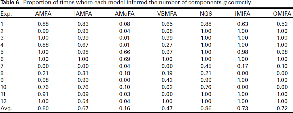
Each method’s ability estimates for inferring the given criteria correctly, obtained by fitting a Rasch model for each of the criteria.
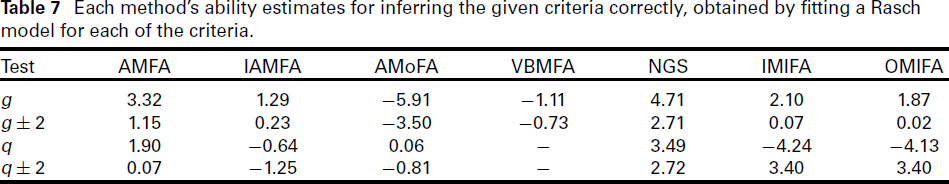
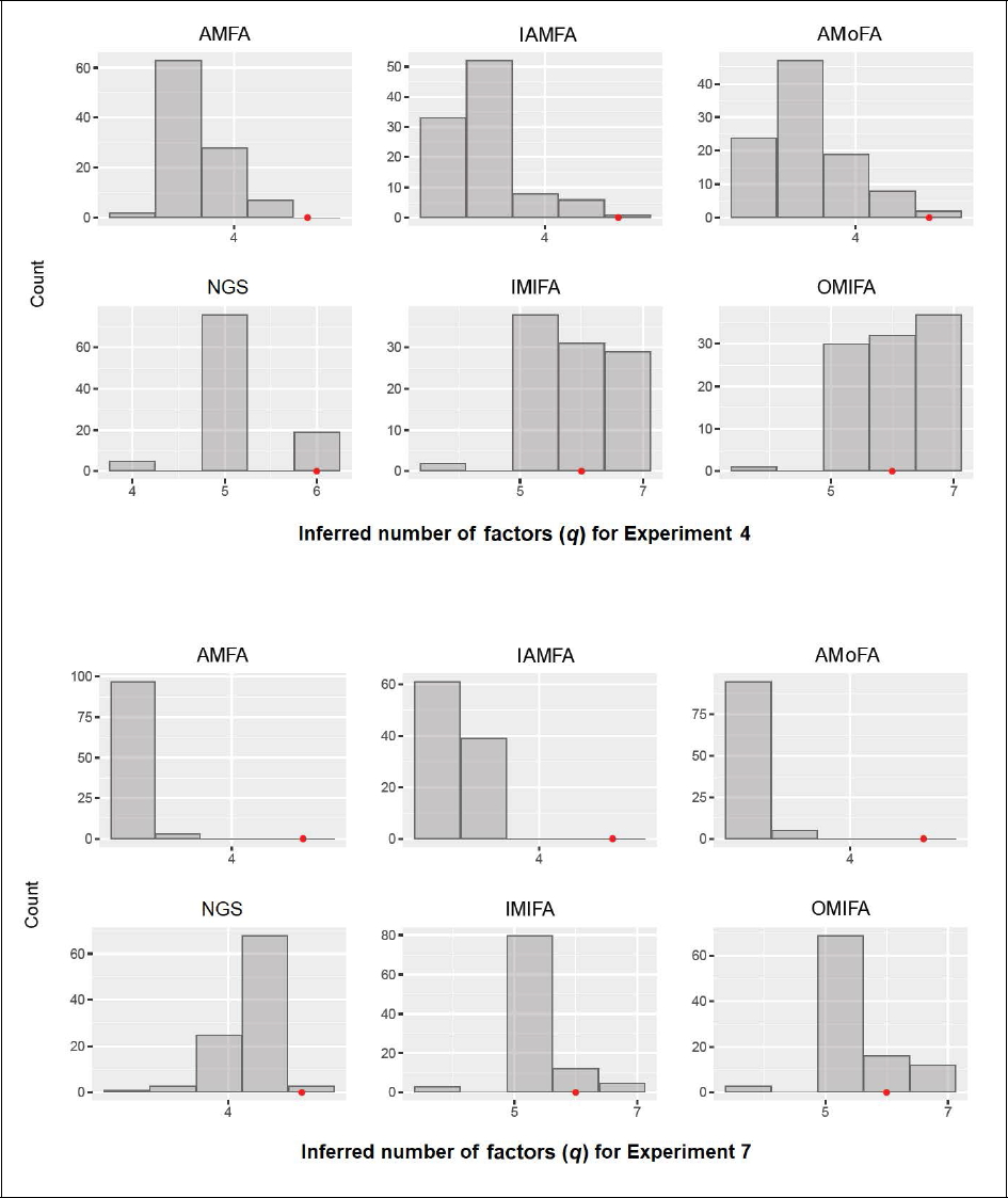
It can be observed from Table 8 that all methods struggled with Experiments 4 and 7. The number of factors were q = 6 in both cases. Figure 2 indicates that AMFA, IAMFA, AMoFA, and NGS tended to underestimate the true number of factors. This was also true for IMIFA and OMIFA in Experiment 7, although to a lesser extent. In this case, the modal number of inferred factors was five for both methods. These two experiments were also the only experiments where AMFA was unable to correctly infer q to within an error of 2 in all trials (see Table 9). Both AMFA and IAMFA almost always underestimated q in these settings, which may suggest that the technique for inferring q (3.1) is less accurate as the number of factors increases. The AMoFA method shows similar pattern, performing reasonably well when q = 1 and q = 3, but very poorly when q = 6. This may suggest its performance scales poorly as q increases.
The Rasch ability estimates in Table 7 support our observations above. We see that NGS has the highest ability estimate for inferring q exactly, whereas IMIFA and OMIFA were ranked equal best when inferring q to within an error of 2. Excluding the NGS, overall AMFA performed best among the methods considered.
In addition, we investigated whether the accuracy of the inferred g had an impact on how well q is inferred. To pursue this, we examined the proportion of times q is inferred correctly given that g has been correctly inferred. For AMFA, IAMFA, NGS, and IMIFA, only minimal increase was observed in the proportion of correctly inferred q. For OMIFA, a slight decrease was observed. However, for AMoFA, the proportion almost doubled. This is likely attributed to AMoFA’s poor ability to infer g correctly. It often drastically overestimates g, resulting in a very different clustering than the true one. On the other hand, if g was provided or estimated correctly, then the inference for q appears to be quite accurate.
Inferred number of factors q for Experiments 4 and 7. The position of the red dot indicates the true number of factors.
Proportion of times where each model inferred the number of factors q correctly.
This study provides a systematic comparison of methods for automatically inferring the number of components (g) and factors (q) in Mixtures of Factor Analysers (MFA) models, including Naive Grid Search (NGS), AMFA, AMoFA, VBMFA, OMIFA, IMIFA, and the proposed IAMFA. We evaluate their performance across a diverse range of settings and in terms of clustering accuracy, model selection, and computational efficiency. The insights from this comparative study provides helpful guidance for automated model selection and are relevant for applied fields such as biomedical research, finance, image processing and social sciences. For example, MFA are frequently used for dimensionality reduction in genomic studies, disease subtyping, and medical imaging.
Our findings indicate that, apart from NGS, AMFA consistently performed best across most evaluation metrics, particularly in terms of model selection accuracy. OMIFA and IMIFA also demonstrated strong performance. IAMFA, while not the top-performing method, provided a balance between computational efficiency and model selection accuracy, making it a viable alternative for applications where exhaustive search methods like NGS are computationally prohibitive. In contrast, AMoFA and VBMFA exhibited the weakest overall performance in these experiments.
A key challenge identified is the computational burden of methods that iteratively refine model complexity. While IAMFA improves on exhaustive search, it still requires iterative component splitting and parameter estimation, which can be costly for high-dimensional data. Scalability remains an issue for even the best-performing methods as dimensionality and sample size increases, highlighting the need for more efficient inference techniques.
Given the strong performance of Bayesian methods such as OMIFA and IMIFA, future work could explore Bayesian adaptations of IAMFA and AMFA, using nonparametric priors and variational inference techniques to improve flexibility and robustness in inferring g and q. Enhancing computational efficiency, particularly for high-dimensional data, is also of interest for future research.
Footnotes
Declaration of Conflicting Interests
The authors declared no potential conflicts of interest with respect to the research, authorship and/or publication of this article.
Funding
The authors received no financial support for the research, authorship and/or publication of this article.
Supplementary materials
Appendix
References
Supplementary Material
Please find the following supplemental material available below.
For Open Access articles published under a Creative Commons License, all supplemental material carries the same license as the article it is associated with.
For non-Open Access articles published, all supplemental material carries a non-exclusive license, and permission requests for re-use of supplemental material or any part of supplemental material shall be sent directly to the copyright owner as specified in the copyright notice associated with the article.