
Abstract
Bayesian structured additive quantile regression is an established tool for regressing outcomes with unknown distributions on a set of explanatory variables and/or when interest lies with effects on the more extreme values of the outcome. Even though variable selection for quantile regression exists, its scope is limited. We propose the use of the Normal Beta Prime Spike and Slab (NBPSS) prior in Bayesian quantile regression to aid the researcher in not only variable but also effect selection. We compare the Bayesian NBPSS approach to statistical boosting for quantile regression, a current standard in automated variable selection in quantile regression, in a simulation study with varying degrees of model complexity and illustrate both methods on an example of childhood malnutrition in Nigeria. The NBPSS prior shows good performance in variable and effect selection as well as prediction compared to boosting and can thus be recommended as an additional tool for quantile regression model building.
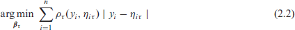
Introduction
In standard regression methods, it is usually the location parameter—very often the mean—of an outcome of interest conditioned on a set of explanatory covariates that is in focus of the estimation procedure. Of course, if the outcome is not characterized sufficiently well by the global conditional location parameter, there exist plenty of methods to also explain other global parameters of the outcome by covariates such as the scale, for example, variance, or shape, for example, skewness, parameters by means of distributional regression a.k.a. general additive models for location, scale and shape (GAMLSS, Rigby and Stasinopoulos, 2005).
While this works perfectly well for outcomes following a known distribution, the task becomes challenging when the distributional form of the outcome violates model assumptions or when it is obvious that there is no global effect to be expected for a specific parameter, but locally there clearly is, for example, for specific quantiles of the outcome, and the task is to quantify that, too. Another drawback of distributional regression is the non-intuitive interpretation of the resulting coefficients, which are—with the exception of the identity link—subject to a distribution-specific link function. In these cases, it helps to consider model types that look beyond the estimation of specific distributional parameters (Kneib, 2013; Kneib, Silbersdorff, and Säfken, 2021). When the form of the outcome is impossible to describe by common modelling distributions, the focus is on quantifying the effects on outliers of the outcome and/ or straightforward communication of the results is necessary, then a suitable regression type is quantile regression first introduced by Koenker and Bassett Jr (1978).
Quantile regression works without parametric distributional assumptions on the outcome and yields potentially non-linear effects for a specific quantile of the outcome conditional on a set of covariates by weighting the outcome accordingly and employing linear programming (Koenker, Ng, and Portnoy, 1994). More flexible models are possible when using other estimation approaches such as Bayesian structured additive quantile regression (Waldmann, Kneib, Yue, Lang, and Flexeder, 2013) or statistical boosting for additive quantile regression (Fenske, Kneib, and Hothorn, 2011). Another challenge for correct modelling is the selection of informative variables. Many different approaches exist for mean regression and have been adapted to suit quantile regression. The LASSO features prominently as a methodological vehicle (Tibshirani, 1996) in variable selection for quantile regression: Koenker et al. (1994), Koenker (2005) and Belloni and Chernozhukov (2011) propose penalized splines in particular L1-penalized splines. Both Wu and Liu (2009) and Lv, Zhang, Zhao, and Liu (2015) use adaptive LASSO; the former in combination with a smoothly clipped absolute deviation (SCAD) function. Zhao and Lian (2016) used group SCAD instead for variable selection, while Ying Sun and Fuentes (2016) applied fused adaptive LASSO in spatial-temporal quantile regression. Sherwood and Maidman (2022) discuss variable selection via SCAD and LASSO in high-dimensional data.
Other methods for variable selection in quantile regression use, for example, a combination of the L0- and L1-norm (Dai, 2023), employ copulas (Fu et al., 2023) or use an information criterion (Eun Ryung Lee and Park, 2014). And Jiang, Bondell, and Wang (2014) proposed a fused penalty to enable variable selection with simultaneous estimation of quantiles and Bar, Booth, and Wells (2023) applied expectation maximization (EM) with weighted least squares to achieve variable selection.
While the previous publications used linear programming in one form or another in their algorithms, there exist also machine learning approaches to variable selection in quantile regression. Meinshausen (2006) established quantile regression forests, Fenske et al. (2011) expanded additive quantile regression to gradient boosting and both He, Qin, Wang, Wang, and Wang (2019) and Liu, Chen, Liu, Qin, and Fars (2023) suggested LASSO-penalized quantile regression neural networks.
In Bayesian quantile regression, the Bayesian equivalent of LASSO (Park and Casella, 2008) is quite popularly employed for variable selection (Waldmann et al., 2013; Alhamzawi, 2015; Shiyi Tu and Sun, 2017; Benoit and Van den Poel, 2017). Other possibilities include indirect variable selection by using the SavageDickey density ratio on the Bayes factors of proposal models (Oh, Choi, and Park, 2016), the proposal of a prior for model selection (Alhamzawi and Yu, 2013) and the usage of spike-and-slab priors in the form of stochastic search variable selection (SSVS) on the model coefficients (Alhamzawi and Yu, 2012; Chen, Dunson, Reed, and Yu, 2013) or on indicator variables (Kedia, Kundu, and Das, 2023).
SSVS spike-and-slab priors for variable selection were first discussed by Mitchell and Beauchamp (1988) and George and McCulloch (1993). They apply a spike-and-slab prior directly on the regression coefficients. When modelling a non-linear effect the respective function can be represented as a basis expansion of the variable of interest with a set of corresponding coefficients and in order to decide on the inclusion of this function in the model, the entire set of coefficients needs to be considered. Ishwaran and Rao (2005) enabled this by applying a spike-and-slab prior to the variance of the coefficients instead of the scalar coefficients themselves. Many variations of this approach exist—see, for example, Panagiotelis and Smith (2008), Zhu, Vannucci, and Cox (2010) or O’Hara and Sillanpää (2009) for a review—but deviations from Gaussian models and/ or variations in the priors to fit the required model suffer from poor mixing (Zhu et al., 2010; Scheipl, Fahrmeir, and Kneib, 2012). In order to improve the mixing properties, Scheipl et al. (2012) proposed the peNMIG spike-and-slab prior for function selection in structured additive regression based on parameter expansion into an importance parameter and standardized coefficients (Gelman, van Dyk, Huang, and Boscardin, 2008). Similar, yet different, is the approach by Klein, Carlan, Kneib, Lang, and Wagner (2021), who proposed the Normal Beta Prime Spike and Slab (NBPSS) prior. In contrast to the peNMIG prior, which relies on the mixed-model-decomposition of effects and a bimodal prior for the standardized coefficients, it uses sparse design matrices resulting in faster computation times and enables samples from the full posterior instead of ones biased towards one of the modes. The NBPSS prior further enables discriminating between a linear and a non-linear component of an effect. While also Guo, Jaeger, Rahman, Long, and Yi (2022) address the problem of selecting the functional form of an effect, they only select non-linear effects once their linear components have been selected first. Thus, their approach might miss non-monotonic functions of variables, whereas function selection with the NBPSS prior does not.
Given the favourable properties of the NBPSS prior we are interested in its extension to a quantile regression context and its variable selection performance therein. In order to do this the methodological background of both Bayesian quantile regression and the NBPSS prior are explained in Section 2. We then apply the NBPSS prior in a simulation study to a set of different models varying in complexity and compare the results to other variable selection mechanisms for quantile regression in Section 3. Section 4 illustrates the application of both approaches to an example of childhood malnutrition in Nigeria and Section 5 summarizes our findings and gives an outlook for possible future developments.
Methods
Traditionally regression models focus on modelling the conditional mean of the outcome given the regressors. The resulting model for the mean might, however, not apply to the more extreme observations. A solution to that is quantile regression, which regresses a specific conditional quantile of the outcome instead of the conditional mean.
Bayesian quantile regression
In quantile regression, the model specification takes the form

where
with
and n denoting the number of observations.
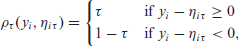
The traditional method of solving (2.2) is by linear programming (Koenker and Bassett Jr, 1978). In order to estimate quantile regression under a Bayesian framework, that is, perform inference of the posterior distribution of the parameters of interest
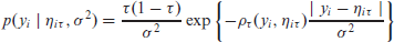
with
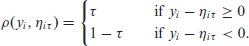
Even though the ALD is an appropriate distribution to represent y in a Bayesian quantile regression setting, it contains an absolute value with undesirable differentiability properties. Fortunately, it can be expressed as a scale mixture of normal distributions with different variants proposed by Kozumi and Kobayashi (2011) and Yue and Rue (2011). For us, the latter is of interest, which uses the formulation

with

While (2.1) illustrates quantile regression with linear effects, the predictor
with
linear effects
non-linear effects given by functions
spatial relation
random effects
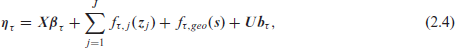
Rewriting equation (2.4) in matrix notation yields

where
For the effects stated above,
For Bayesian estimation of the model as given in (2.3) with the predictor as given in (2.5) we require priors for
where
The prior for the coefficients

For linear (i) and random effects (iv)
Since we are not just interested in inference on the posterior distributions of the effects, but also in automatic function selection and effect decomposition as outlined in the introduction, the priors for the quantile specific effects
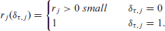
Inclusion of the correct effects in a regression model is paramount. Otherwise the estimates will be biased and the prediction performance will suffer. To achieve this in a Bayesian setting mixture priors with spike and slab components of the form

are applied with hierarchically specified inclusion probability

where
While originally spike and slab priors applied a mixture of normal distributions as prior for the coefficients (SSVS, George and McCulloch, 1993), contemporary spike and slab priors use a Normal Mixture of Inverse Gamma (NMIG) distributions on the variance of the coefficients (Ishwaran and Rao, 2005; Konrath, Kneib, and Fahrmeir, 2008). If effect selection is to include non-linear effects as well, approaches rely on re-parametrization of the effects and apply the prior to a specific parameter of the resulting term (importance parameter) as in parameter-expanded NMIG (peNMIG, Scheipl et al., 2012) and NBPSS (Klein et al., 2021).
This re-parametrization of an effect for the NBPSS prior is such that in the quantile regression setting

holds. The scalar
Consider again the generic and thus flexible prior given in (2.6). With the re-parametrization in (2.8) this prior changes to

In order to ensure identifiability and propriety of the prior Klein et al. (2021) choose the constraint
This specific type of constraint matrix further enables the decomposition of a non-linear effect

This allows to decide whether to include a covariate in the model at all, whether its effect is purely linear or if an additional non-linear effect component needs to be considered as well.
The actual variable or effect selection then happens by imposing a spike and slab prior on the squared importance parameter
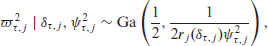
For indicator
When applying the NBPSS prior the choice of the hyperparameters
The graphical display of the employed prior hierarchy is in the supplementary material (Section 1).
In order to put the focus of this article—effect selection in Bayesian quantile regression via the NBPSS prior—in context, we will address other methods for variable selection in quantile regression.
Apart from the NBPSS prior, of the presented alternatives for variable selection in quantile regression only the Bayesian LASSO as used by Waldmann et al. (2013) and gradient boosting for quantile regression by Fenske et al. (2011) are to the best of our knowledge able to estimate structured additive quantile regression models with non-linear and in particular spatial effects.
Simulations
Setup
When it comes to effect selection in quantile regression two scenarios appear relevant: (I) A particular variable either has an effect across all quantiles (informative) or not (non-informative) and (II) a particular variable has an effect on a specific quantile (quantile specific informative), but not on others (quantile specific non-informative). Ideally an effect selection mechanism would be able to discriminate both scenarios and in order to examine whether the NBPSS prior is such a mechanism we will conduct a two-fold simulation study. Part I considers informative vs. non-informative variables and Part II in addition features quantile specific informative vs. non-informative variables. For comparability reasons, we will keep Part I as close as possible to the simulation study by Klein et al. (2021).
Thus, the performance of the NBPSS prior is assessed via its overall accuracy in effect selection as well as its resulting prediction performance and benchmarked against established variable selection mechanisms for quantile regression, that is, Bayesian LASSO as implemented in
Part I: (Non-)informative variables in homo- and heteroscedastic models
For Part I, we replicate several parts of the simulation study conducted by Klein et al. (2021). These include homoscedastic Gaussian and heteroscedastic Gaussian location-scale models. All covariates will be standardized. All in all 16 independent variables x will be simulated according to a uniform distribution U−2,2 and as effects four different functions are specified:
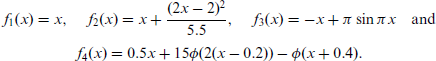
The predictor of the mean
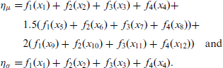
Moreover, the generated data will feature a spatial variable alternating between an informative and a non-informative effect, which will be added to both predictors in the informative cases. The Gaussian models are then simulated from

and the Gaussian location-scale models from

Thus the Gaussian models from (3.1) and the Gaussian location-scale models from (3.2) are identical except for their variance.
To account for estimation complexity due to sample size the Gaussian models are tested on n = 200 and n = 1000 observations and the Gaussian location-scale models on n = 1000 and n = 200 observations. Predictions are performed on n predict = 5000 new observations. Each combination of the above is repeated R = 100 times. Further, to examine sensitivity as to the choice of hyperparameters prior elicitation with the help of the R package sdPrior is carried out with possible combinations of a = 0.05,0.1,0.2 and c = 0.1,0.2.
Part II: Quantile specific (non-)informative variables in heteroscedastic models
Part II of the simulation study will focus on a spatial Gaussian location-scale model with n = 1000 observations and two variables only informative for specific quantiles. The data generation mechanism is the same as for Part I, as is the prediction logic. The predictors take the forms
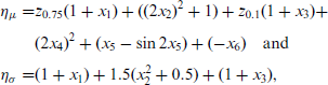
where

While the model simulated in (3.3) is also a Gaussian location-scale model, it differs from (3.2) in the function that links the predictor
For estimation we consider a set of seven quantiles
The results presented here only include the methods 'NBPSS' and 'gradient boosting', since the Bayesian LASSO for geoadditive quantile regression despite it being mentioned in (Waldmann et al., 2013) is not available in
Part I: (Non-)informative variables in homo- and heteroscedastic models
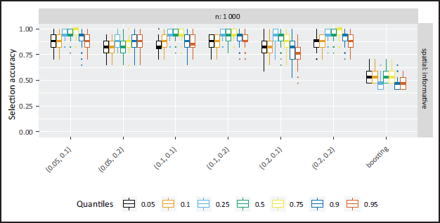
The accuracy of effect selection for the homoscedastic models of Part I is in general very high for the NBPSS prior (Figure 1). This improves further with larger sample sizes. While in the non-spatial case effect selection is more precise towards the inner quantiles, this effect vanishes in the spatial case. This is due to the spatial effect being wrongly selected in the outer quantiles in the non-spatial case. This to a certain degree is a result of decreased data density caused by the weighting step of the scale mixture representation of the observations during estimation as pointed out before. The results also indicate a sensibility of the NBPSS prior towards the chosen hyperparameters suggesting that different combinations of α and c (see Section 2.3) lead to more conservative or liberal selection of variables. Notably a larger probability α influences the selection of non-informative effects and a larger threshold c influences the deselection of informative variables. Detailed figures on the inclusion probability can be found in the supplementary material (Section 4). On a global level, however, this only influences the overall accuracy when α is chosen relatively small and c larger in comparison (or vice versa).
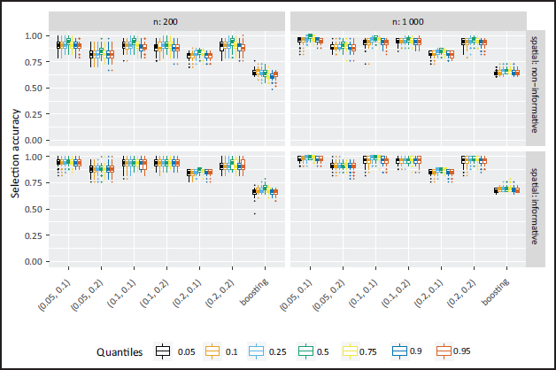
The boosting results show lower selection accuracy in all homoscedastic cases. The reason lies with the high selection frequency of the non-informative variables, incorrect selection of non-linear components of strictly linear effects as well as the frequent selection of a spatial effect in non-spatial cases. For further information, the selection frequencies are depicted in more detail in the supplementary material (Section 4.4).
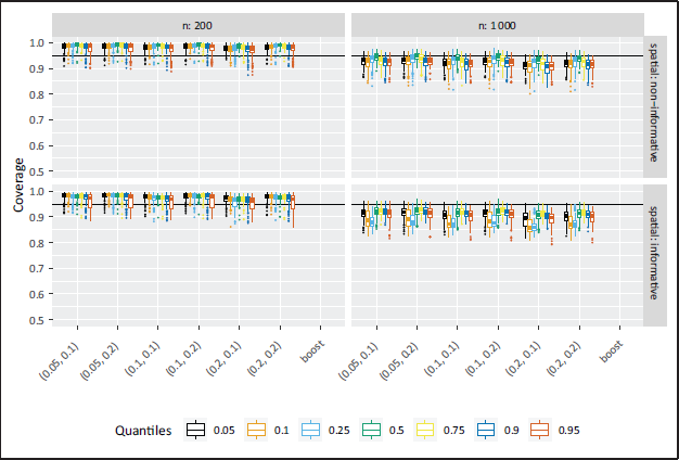
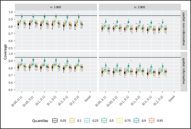
In terms of estimation accuracy, the Bayesian and the boosting approach yield similar values of mean-squared error (MSE) and bias, the 95%-coverage values for the Bayesian results are higher for the inner quantiles (Figure 2). It became relevant throughout the analysis to also consider those parameters in the evaluation of the results. But since they were not planned to be included, theyapart from the depiction of the coverage—can be found in the supplementary material Section 5.
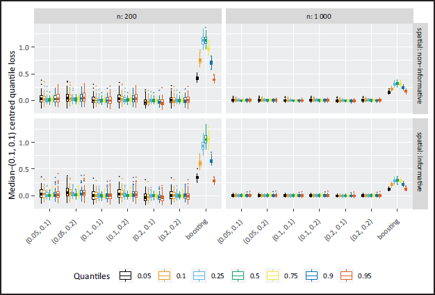
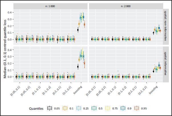
When it comes to prediction performance, the median-(0.1,0.1) centred quantile loss is in general less for the NBPSS prior than for boosting, yet the discrepancy shrinks with increasing sample size (compare Figure 3). The boosting performance can be traced back to the incorrect effect selection. In addition, the NBPSS prior shows more variability towards the outer quantiles, while the behaviour is inverted for boosting, which has higher variability towards the inner quantiles. For the Bayesian approach, the higher variability can be traced back to the more pronounced weighting of the data in the outer quantiles making estimation a little less stable and eventually being reflected in the prediction. In contrast to the selection accuracy, the choice of hyperparameters does hardly impact the quality of the prediction.
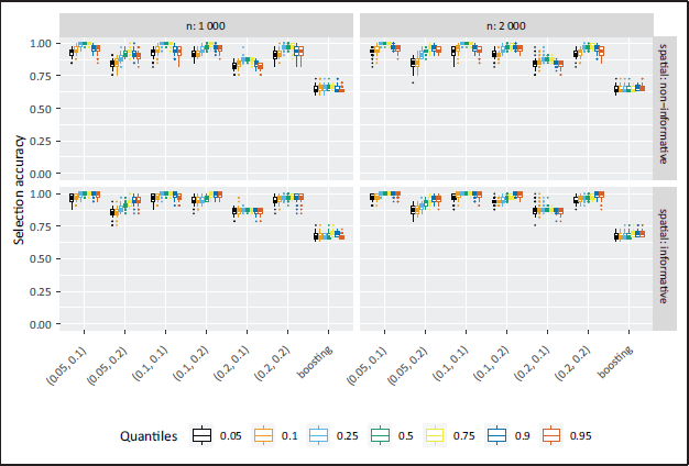
For the heteroscedastic models a very similar picture is evident in terms of selection accuracy. The NBPSS prior yields high selection accuracy with slight drops towards the outer quantiles in the non-spatial case (see Figure 4) due to incorrect selection of the spatial effect as well as the artificial imbalance induced by weighting the data. What also becomes evident is that for the heteroscedastic effects of variables x1 to x4 the selection accuracy is quantile specific, which seems incorrect at first, but is indeed the desired behaviour. For certain quantiles, the effects of those variables are flat and rather close to zero (illustration in the supplementary material Section 3) and in consequence, effect selection is lower. This is the case for quantiles
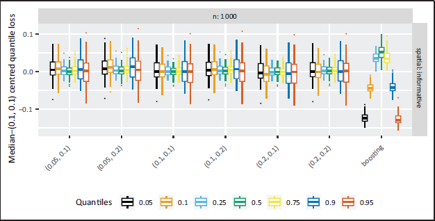
Despite the additional complexity in the simulated data, the prediction performance in the heteroscedastic models is improved due to larger samples, that is, the median-(0.1, 0.1) centred quantile loss is smaller than in the homoscedastic cases (see Figure 6). The median-(0.1,0.1) centred quantile loss generated by the boosting results is again higher than in the NBPSS prior results, but similar to the homoscedastic case the difference between the two methods decreases with increasing sample size. The increased sample size also seems to have a homogenizing effect on the variability in results across the quantiles: For the NBPSS the outer quantiles are still more volatile than the inner ones and vice versa for boosting, but this balances out with increasing sample size.
Part II: Quantile specific (non-)informative variables in heteroscedastic models
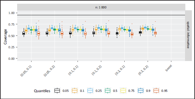
In Part II of the simulation study featuring quantile specific non-informative variables the overall accuracy is again relatively high as can be seen from Figure 7, but coverage appears low (Figure 8). The accuracy results are expected to drop towards the outer quantiles, since the effect of x1 was non-informative on the 25%-quantile and the effect of x3 on the 90%-quantile. As a consequence, the effects of the neighbouring quantiles are very small and the NBPSS prior shows expected selection and deselection for the relevant quantiles. In contrast, the boosting approach overall shows a weaker selection accuracy and the driving reasons behind this compared to the Bayesian outcomes is high selection of non-informative variables and effects. Illustrations of the quantile-specific non-informative effects, inclusion probabilities and selection frequencies are provided in the supplementary material Figures 3, 12 and 15.
Compared to Part I the prediction quality for the boosting results is closer to the Bayesian results in Part II, as can be seen in Figure 9. For boosting the median-(0.1,0.1) centred quantile loss is less for the more extreme quantiles than for the NBPSS results, and vice versa for the inner quantiles. The prediction variability is again higher in the outer quantiles for the Bayesian results and higher in the inner quantiles for the boosting results. The former can as before in Part I be traced back to the weighting of the observations as part of the scale mixture representation of quantile regression. For the NBPSS prior this behaviour is independent of the hyperparameters.
Compared to the previous publication on variable selection with the NBPSS prior in distributional regression (Klein et al., 2021), the results for quantile regression seem to fall behind expectations especially when measured by ‘selection accuracy’. But then the intention of quantile regression is to model an outcome locally and a local effect might differ substantially from a global effect (as yielded by distributional regression). As the heteroscedastic cases of Part I and the specifically designed Part II of the simulation study have shown, a particular effect might be more or less smooth or (close to) zero altogether for a specific quantile.
This leads to the question: When can a predictor on a specific quantile be considered correctly specified? On the one hand, it is desirable that all components are selected despite being very small, which is especially important in the setting of a simulation study with the aim of measuring the quality of the effect selection properties. At the same time, it is to be questioned whether other variable selection mechanisms might achieve such a task (potentially also in other regression settings) and whether selection based on the posterior inclusion probability alone is sufficiently precise in these cases. The latter can be complemented by taking also the effect size and its deviation from the true effect into consideration as we did throughout the course of this simulation study with the common metrics MSE, bias and coverage (provided in the supplementary material). On the other hand is the argument of parsimony of the final model for a specific quantile, against which it might be argued that the simpler model, for example, a very small effect being left out or a slightly non-linear effect being modelled as linear only, is sufficient to describe the conditional quantile of the outcome. Following this thought the posterior inclusion probability would be well suited to determine the predictor for a specific quantile and can be recommended in application settings.
Identifying predictors of chronic malnutrition
In low- and middle-income countries malnutrition remains a problem, especially so when affecting children. The Demographic and Health Surveys (DHS) Program (
In general, it makes sense to distinguish between acute malnutrition and chronic malnutrition. A common measure for the latter is stunting, that is, insufficient height for a child's age. It is defined as a Z-score standardizing the actual anthropometric measurement by a reference population and its calculation follows the WHO Recommendations for data collection, analysis and reporting on anthropometric indicators in children under 5 years old.
Now quantile regression especially of the lower quantiles is particularly well suited for analysing the topic of malnutrition since it allows to focus on the more extreme observations that represent varying stages of malnutrition better than is possible when regressing the mean. In addition, the broad variety of topics covered in the DHS Program allows us to explore the question of which indicators predict more severe cases of childhood malnutrition measured as the 5% and 10%-quantile of stunting.
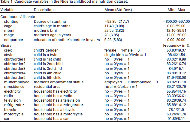
In terms of country, our analysis will focus on Nigeria, which still exhibits distinct sociodemographic inter-regional disparities. For comparability reasons with an earlier analysis on this topic by Klein et al. (2021), we will focus on data from 2013 and the same candidate variables for selection as given in Table 1. After cleansing (removing outliers and inconsistent values), 8 005 completely observed cases remain.
Candidate variables in the Nigeria childhood malnutrition dataset.
The analysis will focus on the 5%- and 10% -quantile to capture the more severe cases of malnutrition and the median to allow for comparison with mean regression as performed in Klein et al. (2021). We specify the continuous variables cage (child's age in months), mbmi (mother's BMI), mage (mother's age in years) and edupartner (education of mother's partner in years) as smooth effects decomposed into their linear and their non-linear component. These variables are centred before the analysis to increase the stability of the algorithm. The remaining binary variables enter as exclusively linear effects. As a benchmark for variable selection in quantile regression we will compare NBPSS results to results from gradient boosting for quantile regression (package
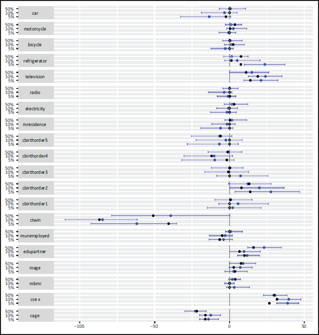
Figure 10 shows the exclusively non-linear part of the effects of the quantitative variables on stunting for the different quantiles under analysis together with the boosted results and Figure 11 depicts the posterior means and 95%-credible intervals of the linear effects of the quantitative and binary variables together with their boosted counterparts. A depiction of the re-composed smooth effects is provided in the supplementary material (Section 6).
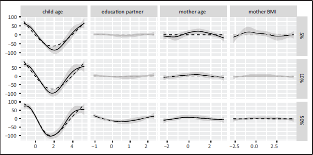
Inspecting the smooth effects it becomes clear that the results of both methods are very similar. The NBPSS prior selected most of the smooth effects across the quantiles with the exception of the mother's BMI for the 10%-quantile and the median and the education in years of the mother's partner for the 5% - and 10%-quantile. Gradient boosting performed a similar selection, but the mother's BMI for the median, the mother's age not for the 10%-quantile and the partner's education not at all.
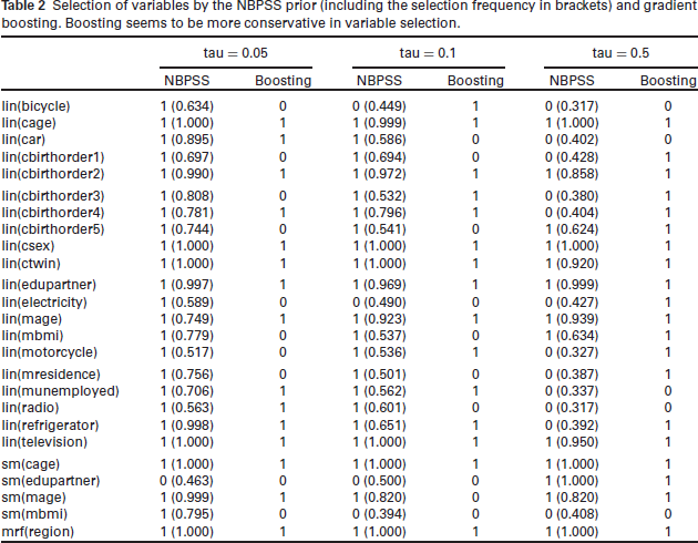
Analogously to the non-linear part, the linear effects yielded by both methods are very similar in magnitude. The only difference between both methods seems to lie in the selection of variables: Gradient boosting tends to select less linear effects than the NBPSS prior at the 5% - and 10% quantile and more at the median (compare Table 2).
Selection of variables by the NBPSS prior (including the selection frequency in brackets) and gradient boosting. Boosting seems to be more conservative in variable selection.
Both algorithms also select the spatial effect for each quantile. Combined with the intercept they show a similar effect with a north-south-disparity (compare Figure 12).
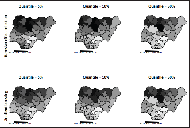
Socio-demographic factors such as the child being a girl, the mother's age or the partner's education have a protective effect on the level of stunting of a child, while the child's age or unemployment of the mother constitute risk factors. Years of partner's education and the mother's age show higher protection in the median, but the child's gender is more protective for the lower quantiles. Interestingly the child's age as a risk factor is more distinct in the median than in the lower quantiles. Moreover, the spatial effect shows a pronounced north-south-disparity with the southern, more urban regions acting as protection against chronic malnutrition. In addition, the living situation of the child plays a role: A refrigerator and television in the household were protective indicators of children's nutritional status especially in the lower quantiles, while other forms of media or electrification didn't play a role. In particular, the latter could be highly correlated to the region the child lives in with the availability of both being higher in the urbanized areas in the south and is thus covered by the spatial effect. Further, the order of birth appears to impact the level of stunting: Being the first or in particular the second child is a protective factor, the risk of stunting rises, however, with increasing order of birth. It is worth noting that this effect is more pronounced for the lower quantiles than it is for the median. Mobility factors don't seem to have a distinct impact on the severity of stunting regardless of the quantile. These outcomes are comparable to the findings in Klein et al. (2021).
To make the findings of the data example reproducible, the code used for the analysis can be found on github on ‘/arappl/Nigeria’.
The aim of this study was to examine the NBPSS prior as an effect selection mechanism in Bayesian structured additive quantile regression and compare the outcome to Bayesian LASSO and gradient boosting for quantile regression. This was performed through a simulation study and illustrated by an example of childhood malnutrition in Nigeria. Results for Bayesian LASSO are not included, since this method was not available within the stated platform.
When it comes to variable selection in quantile regression, two scenarios are relevant: A variable might not be informative on the entire model or it might not be informative on a particular quantile. Our two-part simulation study accounted for both. The first part was kept close to the original publication of the NBPSS prior to capture various model complexities and it showed that the NBPSS prior outperformed boosting when it came to variable selection. It already became apparent that it is sensitive towards variables having no or a very small effect on specific quantiles, which is desirable behaviour. This was then confirmed in the second part of the simulation study, which in addition also covered variables non-informative on specific quantiles. The NBPSS prior proved its ability to discriminate between the two and yield accurate estimation results. Finally the findings were applied to data on childhood malnutrition in Nigeria and the results of both variable selection mechanisms were encouragingly close and in line with previous research on childhood malnutrition.
What was interesting is that a prediction optimized method such as gradient boosting was outperformed by a Bayesian variable selection mechanism. This said it needs to be noted that gradient boosting for quantile regression was used here in its default settings in order to use an established baseline for comparison and in what for boosting constitutes a rather low dimensional setting. Given that boosting is known to perform stronger in considerably higher dimensional data situations and given the variety of available stopping criteria other than the employed cross-validation the overall performance of boosting in the present case could surely be optimized. An approach to this can be found in Strömer, Staerk, Klein, Weinhold, Titze, and Mayr (2022).
Despite the performance of the NBPSS prior the weights drawn in the MCMC algorithm for Bayesian quantile regression in order to achieve the scale mixture representation is computationally costly and particularly in the outer quantiles several tries may be needed to achieve convergence. This behaviour is amplified by adding a variable selection mechanism such as the NBPSS prior. Furthermore, the selection of variables is sensitive towards the hyperparameters chosen for the NBPSS prior and very small or zero effects are not entirely deselected, but rather shrunken. While this is still acceptable from a statistical perspective, applied researchers might wish for a clear guideline on how to deal with such cases.
This could be achieved by a sensitivity analysis on an informed choice of hyperparameters and handling of very small effect estimations and might be an aspect of future research. Especially with applied researchers in mind a user-friendly solution similar to the
Supplementary material
Supplementary materials for this article are available online.
Supplemental Material for Bayesian effect selection in structured additive quantile regression by Anja Rappl Manuel Carlan Thomas Kneib Sebastiaan Klokman and Elisabeth Bergherr, in Statistical Modelling
Footnotes
Declaration of Conflicting Interests
The authors declared no potential conflicts of interest with respect to the research, authorship and/or publication of this article.
Funding
Thomas Kneib gratefully acknowledges funding from the Deutsche Forschungsgemeinschaft (DFG, German Research Foundation), grant KN 922/9-1. Elisabeth Bergherr gratefully acknowledges funding from the Deutsche Forschungsgemeinschaft (DFG, German Research Foundation), grant BE 7939/2-2.
References
Supplementary Material
Please find the following supplemental material available below.
For Open Access articles published under a Creative Commons License, all supplemental material carries the same license as the article it is associated with.
For non-Open Access articles published, all supplemental material carries a non-exclusive license, and permission requests for re-use of supplemental material or any part of supplemental material shall be sent directly to the copyright owner as specified in the copyright notice associated with the article.