
Abstract
The sparsity-ranked lasso (SRL) has been developed for model selection and estimation in the presence of interactions and polynomials. The main tenet of the SRL is that an algorithm should be more sceptical of higher-order polynomials and interactions a priori compared to main effects, and hence the inclusion of these more complex terms should require a higher level of evidence. In time series, the same idea of ranked prior scepticism can be applied to characterize the potentially complex seasonal autoregressive (AR) structure of a series during the model fitting process, becoming especially useful in settings with uncertain or multiple modes of seasonality. The SRL can naturally incorporate exogenous variables, with streamlined options for inference and/or feature selection. The fitting process is quick even for large series with a high-dimensional feature set. In this work, we discuss both the formulation of this procedure and the software we have developed for its implementation via the
Introduction
In time series analyses, the comfort of asymptopia, where our series of interest has infinite observations and can be suitably characterized by a small set of endogenous parameters, can become a fool’s paradise. With freely available statistical and computational tools built for high dimensional problems, those who dare to venture away from conventional asymptotic theory may be able to build better predictive models and learn more richly about causal mechanisms at play in a data-saturated world.
In this work, we will show how new applications of existing statistical theories and tools can be utilized in time series analyses to produce better inferences and forecasts, focusing on scenarios with complex seasonal patterns and exogenous covariates. We start by describing the background and reviewing existing methods in this space, including common means of modelling seasonal time series data. We then illustrate how ranked-sparsity-based tools such as the sparsity-ranked lasso (SRL) can be extended to outperform existing methods, proceeding through both the formulation of the procedure and the software we have developed for its implementation via the
Background
In this section, we will describe common models for seasonal time series data, several candidate fitting procedures, and several considerations for choosing parameters for these models.
Autoregressive models
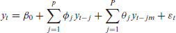
Consistent and continual data collection is beginning to pervade our lives in unprecedented and unexpected ways. Time series data, where one variable is measured many times at regular intervals, is ubiquitous. A measurement in the present usually depends on its past (say,

where after controlling for the autocorrelation in the conditional mean structure, the residuals are assumed to be independent and normally distributed about zero.
One common question is the best way to select
A time series may also be expected to follow some pattern (or patterns) of seasonality; for example, online searches related to the National Football League will peak during the football season every year. For this reason, it is important that this seasonality be accommodated in the autoregressive model. Let
where again, the
The benefit of representing the AR and SAR models in this linear model form is that it becomes clear how least-squares (or some other estimation technique) can be used to estimate the AR parameters. However, there are also models that cannot be easily represented by this lagged model form for instance, those with moving average (MA) components. The now-ubiquitous autoregressive integrated moving average (ARIMA) model can handle moving average terms as well as differencing, which may be advisable if the time series is not stationary (Cryer and Chan, 2008).
Existing methods for order selection
For ARIMA models, it is common practice to use a likelihood-based estimation procedure to fit models with potentially both AR and MA terms. After a set of candidate models has been fit, an information criterion, such as Akaike’s Information Criterion (AIC), its small sample corrected version (AICc), or the Bayesian Information Criterion (BIC), can be used to select an optimal model order. This process is implemented automatically in the
If only AR and SAR models are considered, then the Least Absolute Shrinkage and Selection Operator (the lasso) (Tibshirani, 1996) can be used to estimate the coefficients and select an optimal
Complications in modelling periodic patterns
In the modelling of time series that exhibit prominent recurring patterns, it can be important to distinguish between cyclic and seasonal periodicity. Cycles refer to patterns arising from variable periodicity whereas seasonality refers to patterns arising from fixed periodicity. (See, for instance, Hyndman and Athanasopoulos, 2018). Often, cyclic time series can be effectively modelled using traditional, lower-lag autoregressive terms. With seasonal time series, the length of the fixed period m is generally implied by the context of the underlying phenomenon. For example, Shumway and Stoffer (2000) describe an environmental series called the Southern Oscillation Index (SOI) that is measured monthly for 453 months ranging over the years 1950-1987. This series exhibits a strong yearly period
For non-cyclical seasonal time series, especially when the data are collected at very short intervals relative to the length of the series, multiple modes of seasonality may exist. If the series is modelled as an autoregression with a large value of
A separate issue in modelling non-cyclical seasonal time series may occur when the relationship between the seasonal period and the sampling rate is not well-understood. For example, the sound energy from a recorded song likely exhibits seasonality owing to the song’s natural tempo, however unless song’s tempo is documented, the seasonal period cannot be connected to the sampling rate of the recording. In such cases, it can be difficult to specify a definitive value for
Potential solutions
In modelling seasonality in the AR framework, a valuable technique involves the inclusion of nearby seasonal lags as additional parameters:

Here, we employ the notation
If we use the lasso to fit this model, it will naturally estimate some coefficients to be zero, so we can re-frame this selection problem, setting

In words, instead of assuming there will be structural gaps in the important lags in the SAR model, we parametrize every coefficient up through the maximum possible lag and will take care (in the following section) to ensure the solution is sparse and resembles the SAR model. This formulation means that a very high order AR model could be selected, depending on the expected pattern (or patterns) of seasonality. However, if the primary goal is prediction in large-sample settings, there is no downside to selecting a high order model (other than potentially adding in a lot of noise, which hopefully can be avoided with the use of the lasso and an effective model selection criterion).
Another popular method for fitting seasonal time series with multiple modes of seasonality is called the TBATS method (which stands for ‘trigonometric, Box-Cox transform, ARMA errors, trend, and seasonal components’) (De Livera, Hyndman, and Snyder, 2011). As with automated-ARIMA, the TBATS method can be implemented efficiently in the
In this section, we show how the SRL can be used in the time series regression framework to fit AR and SAR models quickly, effectively, and accurately, while also optionally accommodating and selecting from a set of important exogenous features.
Dynamic penalty tuning with the sparsity-ranked lasso
When prior informational asymmetry is present among candidate predictors, for instance when selecting from all pairwise interactions and polynomials, Peterson and Cavanaugh (2022) motivated and explored the use of the sparsity-ranked lasso. Its main tenet is that an algorithm should be more sceptical of higher-order polynomials and interactions a priori compared to main effects, and hence the inclusion of these more complex terms should require a higher level of evidence. Otherwise, if interactions and polynomials are treated with ‘covariate equipoise’, algorithms will tend to yield many more false discoveries for interactions and polynomials, which makes models less transparent, harder to communicate, and worse at prediction. The intuition behind the lasso-based implementation of ranked sparsity (the SRL) involves assigning weights to each candidate covariate based on the degree of scepticism that the covariate should in fact enter the model, as illustrated in the expression below:
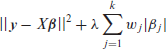
Here,
The SRL is designed to be of use when the assumption of covariate equipoise, defined as the prior belief that all covariates are equally worthy of entering into the model, is not satisfied. In the AR framework, this assumption is definitely not satisfied, and the SRL can address the resulting challenge. Particularly, going from equation (2.1) to equation (2.2) in the previous section is suspect; we have very good reason to believe that the effects on the lags between
Parametrizing scepticism
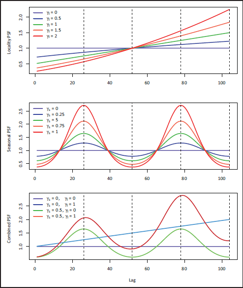
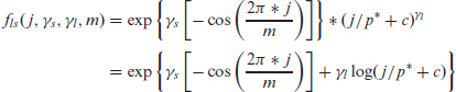
Since we have good reason to believe that recent and seasonal lags are more likely to be important, but we are not certain, we can operationalize this notion using what we call penalty-scaling functions. These penalty-scaling functions, which we denote as

If
Parametrized penalty scaling functions (PSF) for coefficients on lags up to
in a time series SRL setting. The top plot refers to the locality PSF
, the middle plot refers to the seasonal PSF, and the bottom plot is their combined PSF. In the bottom plot,
.
Parametrized penalty scaling functions (PSF) for coefficients on lags up to
in a time series SRL setting. The top plot refers to the locality PSF
, the middle plot refers to the seasonal PSF, and the bottom plot is their combined PSF. In the bottom plot,
.
For the seasonal penalty-scaling function, we use the parameter
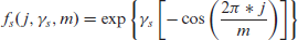
Here
This penalization is visualized for different values of
The parametrically-weighted SRL is especially useful for handling gaps in the AR structure, and it can be straightforwardly extended to considering multiple modes of seasonality. However, the method is not without drawbacks. A minor drawback occurs when the seasonal frequency
We have explored these parametrized penalty-scaling functions and applied them successfully in multiple applications, and will return to them in the simulation section. However, the SRL method that we discuss in the next subsection performs similarly and is more broadly applicable than the parametrized version.
SRL with the partial autocorrelation function
Instead of having a predefined parametrized ranking of scepticism for various lags in a time series model, we could use the data to inform these penalty weights. A useful means to accomplish this is to employ the partial autocorrelation function (PACF), defined as the correlation between
The adaptive lasso (Zou, 2006) involves penalty weights

Here
If there are exogenous covariates, we can include weights for these as well; let
The SRLPAC approach is ideal for modelling time series data with complicated seasonality; it is quick, intuitive, and can be conveniently tuned using AICc or BIC provided the sample size is large, which is typically the case in time series settings. Further, SRLPAC does not require the pre-specification of seasonal modes at all; it does this naturally and automatically using the PACF. Finally, the SRLPACx approach has all the same advantages while also allowing for seamless integration of (possibly very many) exogenous variables.
Generally, the hyperparameter for the lasso (and the SRL) models can be tuned using either information criteria (AIC, BIC, or AICc) or cross-validation (CV). BIC will generally select sparser (lower order) autoregressive models, while AIC, AICc, and CV will attempt to minimize prediction error (typically by allowing more coefficients into the model). Since predictive accuracy is usually of primary importance for time series applications, we recommend using CV or AICc in most cases. With time series data,
Measuring predictive accuracy
In order to measure prediction accuracy in a time series setting, there are many possible options. Since our methods use least squares to fit parameters, we use the root-mean-squared prediction error (RMSPE) and
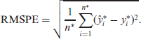
RMSPE is interpretable in the same unit of measurement as the original measurement for
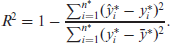
This definition of
The fastTS package
We have developed the
The
Simulation study
Simulation set-up
To demonstrate the performance of our proposed method and its competitors, we have implemented a set of Monte Carlo simulations under controlled settings. We consider five generative data models based on fitted models for the emergency room visit data set described in our application. Briefly, in our application, we suspect multiple modes of seasonality and potentially important exogenous covariate effects which include concurrent hourly temperature and a set of holiday (and day-after holiday) indicator variables. Our main generative settings were designed to capture various degrees of simplicity:
Due to the computational time needed to fit automated ARIMA and TBATS methods, we reduced the sample size considerably to
Data-based generating model parameters for MA-based simulations.
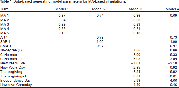
Data-based generating model parameters for MA-based simulations.
To fit simulated data produced from these generating models, we used automated SAR, automated SARx, TBATS, SRLPAR, SRLPAC, SRLPARx, and SRLPACx. We restricted our ARIMAbased methods to AR-only models so that the MA-based true generating models could not be perfectly specified by any of the fitting methods. For the SRLPAR method, we set penalty scaling functions using
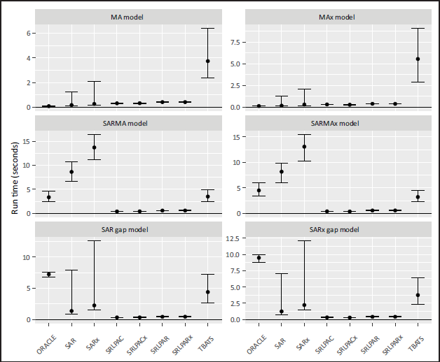
The median and IQR performances and computation times for our simulations are presented in Figures 2 and 3 respectively.
Performance of various fitting methods relative to the oracle (true) model for simulations. A value of 1 indicates that the RMSPE is as good as the oracle fit to the same training data. Points represent medians, and bars represent the interquartile range.
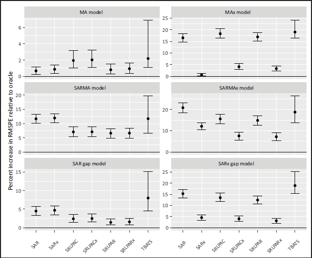
Performance of various fitting methods relative to the oracle (true) model for simulations. A value of 1 indicates that the RMSPE is as good as the oracle fit to the same training data. Points represent medians, and bars represent the interquartile range.
Median computation time for fitting methods to 500 simulated data points. Functions used included the Arima() , auto.arima() , and tbats() functions from the forecast package, and fastTS() function from the fastTS package. Points represent medians, and bars represent the interquartile range.
In the MA(5) data-generating model, SAR- and SRL-based methods perform similarly (with SRLPAC method performing slightly worse than SRLPAR). Models were able to achieve much better predictions when incorporating the exogenous covariates, at which point the difference between SRLPACx and SRLPARx became minor, and both showed a slightly worse performance than the automated SARx model. In the SARMA data-generating model, the TBATS and SAR-based methods performed much worse than those based on SRL. In the SARMAx generating model, the SRLPACx and SRLPARx models performed similarly, better than the automated SARx model, and much better than the other methods which did not account for the exogenous signals. In the SAR gap data-generating models, we see superior performance of the SRL-based methods, with the parametric variant exhibiting slightly better performance than the PACF variant.
The SRL-based methods achieved a very considerable improvement in speed relative to the automated SARx, TBATS, and even the oracle fitting method. The benefits of improved computational speed were more apparent for the more complex data-generating models. For the SAR gap generating model, the automated SAR and SARx fitting methods reflected a high degree of variability in the run times, while the run times for the SRL-based methods were not only fast, but also exhibited little variability.
In short, we have confirmed that the SRL-based methods are well-suited to seasonal data, can fully leverage signal from exogenous features to improve predictions, and are more computationally efficient and consistent than currently available software.
We showcase our methodology in a novel approach to emergency room visit forecasting. For planning purposes, it is highly desirable to accurately forecast the expected number of visits in the emergency room (ER) each hour. Accurate forecasting (and planning) reduces the costs and frustrations associated with having to ‘call-in’ extra help. Previous research has indicated that time series models can be developed and utilized to predict ER visits on the daily time-horizon (Jones et al., 2008). However, these daily forecasts, while informative, are less helpful from a practical standpoint since shifts are typically set for under 12 hours. It is useful to have more granular predictions so that personnel resources can be allocated more efficiently on a shift-by-shift basis. Other research investigating the forecasting of ER arrivals at the hourly level does exist, and mostly utilize seasonal ARIMA models to fit the hourly series for a single ER. A detailed literature review is outside the scope of this manuscript.
In this study, we examine hourly visit counts for the Emergency Department at the University of Iowa Hospital and Clinics (UIHC) from July 2013 to March 2018. Since this is hourly data over a long time span, the sample size in this modelling problem is large
In Figure 4, we indeed observe many modes of seasonality. The most prominent correlation is the
Partial Autocorrelation Function for hourly emergency room arrivals.
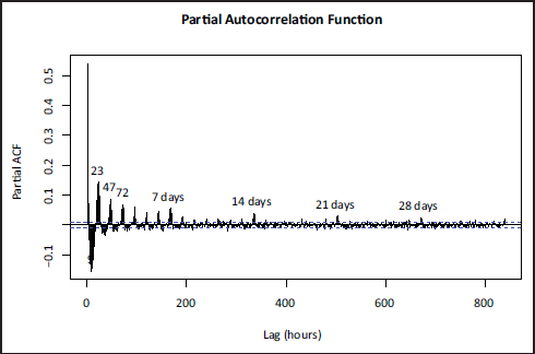
Partial Autocorrelation Function for hourly emergency room arrivals.
We consider monthly effects, holiday effects, and concurrent hourly temperature in Iowa City, Iowa, as exogenous features, unpenalized in the regression. For months and holidays, we used indicator variables to denote month as well as specific holidays, including Christmas, New Year’s Eve, New Year’s Day, Thanksgiving, Independence Day, and Hawkeye game-day (i.e., the day of an Iowa Hawkeye college football game). We also include holiday ‘plus-one’ effects for Christmas and Thanksgiving to examine if there are lingering effects of these major holidays.
Before fitting the models, we divide our sample into a training set (the first 90% of data, 7/1/2023-10/9/2017) and a test set (the final 10% of data through 3/31/2018). Using the training set, we fit the following models:
SRLPAC SRLPAC with exogenous variables (SRLPACx) Automated SARIMA, with TBATS model with daily, weekly, monthly, and yearly frequencies specified:
In addition to computing the metrics outlined in the previous section on the test data, we repeat the fitting process 12 times to calculate the mean computation time (MCT) for each method. For both SRLPAC models, we use AICc to select a value of
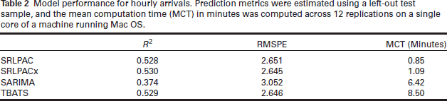
We see in Table 2 that the automated SARIMA approach performed the worst by all measures; it took a relatively long time to run, and the models it produced did not predict accurately. The TBATS method did predict one-step ahead quite well, though it also took much longer to run than either SRLPAC approach. SRLPAC and SRLPACx performed well, both with and without the exogenous variables, the inclusion of which seems to offer a modest improvement in predictive accuracy. The SRL with exogenous variables and TBATS were essentially tied and performed best at one-step predictions.
Model performance for hourly arrivals. Prediction metrics were estimated using a left-out test sample, and the mean computation time (MCT) in minutes was computed across 12 replications on a single core of a machine running Mac OS.
In contrast to TBATS, we can make interpretable inferences regarding the exogenous variables using the SRL-PACx model, where interpretations condition on the rest of the covariates in the model as well as relevant
1
autocorrelation (Figure 5 and Table S3). We find that hourly ER visits exhibit seasonality on a yearly-scale in addition to a very strong positive association concurrent hourly mean temperature; for every 10 degree
Coefficient estimates and 95% confidence intervals for exogenous variables in SRLPAC model. Values refer to the expected change in hourly visits controlling for other factors in the model, including temporal correlation.
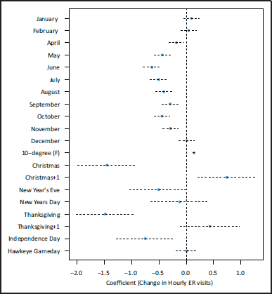
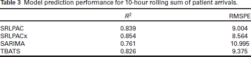
Table 3 shows model prediction performance for how many patients arrived in the ER in a 10hour window. The SRLPAC methods performed similarly to one another with a slight advantage toward the SRLPACx model, with both methods outperforming TBATS and automated SARIMA. This optimal model was able to describe 85.4% of the variation in the 10 -hour rolling sum of ED arrivals. The SRLPACx model’s RMSPE was the lowest; its prediction was on average only about 8.6 patients off of the true value. Figure S1 shows the accuracy of the SRLPACx model in predicting the 10-hour rolling counts. Of note, the SRLPAC and SRLPACx models generated 1- through 10-step ahead predictions in under 5 minutes, while TBATS and SARIMA procedures took considerably longer (2 hours for the TBATS predictions and over 6 days for the SARIMA predictions).
Model prediction performance for 10 -hour rolling sum of patient arrivals.
When time series data exhibit complex and potentially multiple-mode seasonality as well as exogenous covariates, popular existing modelling strategies lack crucial flexibility. We have shown that the sparsity-ranked lasso is adaptable to time series data in several ways. Not only do SRL-based methods rival the predictive accuracy of other state-of-the-art forecasting methods, they facilitate the seamless incorporation of exogenous data and run considerably faster for large data sets. Joining the sparsity-ranked lasso with the partial autocorrelation function (SRLPAC), we were able to accurately forecast the number of patients who would arrive at the UIHC Emergency Department to within an average of about 8.5 patients per 10 -hour time window. We were also able to use the SRLPACx model to make inferences about patterns in the data, finding large associations between ER arrivals and temperature, month, and holidays.
For similar staffing purposes (and more generally), a quantile of the forecast distribution may be preferred to the mean. For this goal, we note that forecasts should theoretically be normally distributed asymptotically, so the analyst could compute prediction intervals using the estimated forecast variance based on its parametric form for an AR model.
Other researchers have shown that SARIMA models are effective in forecasting the number of ER arrivals for daily data, see (Jones, Thomas, Evans, Welch, Haug, and Snow, 2008) for example. However, we have shown that for local hourly data, the SARIMA model does not perform effectively compared to other methods, and the only methods that can predict well and handle exogenous covariates are SRL-based.
We are not the first to apply the lasso in time series applications (e.g. Chernozhukov et al., 2021), though we are unaware of existing methods or software devoted specifically to applying it to seasonal time series. Existing variable selection methods for time series models using information criteria typically make use of recency, dropping older lags first as a part of the tuning process. Relative to this practice, our methods have an advantage when the lag structure includes some kind of ‘delayed effect’ (i.e. there are gaps in the lag structure). We have shown how SRL-based methods can capture this, whereas traditional recency-guided methods using information criteria will not. We expect the SRL-based methods to also well-capture gaps in seasonal lag structures; for example when the first and third seasonal lag are important, but the second one is not.
Although we have only shown empirical evidence in this work, we suspect that the SRL-based methods will perform similarly well for other time series data sets with complex seasonality and/or exogenous features. To this end, we have created the
Footnotes
Acknowledgements
We would like to thank two anonymous reviewers as well as Gary Grunwald for providing vital advice on how to describe the utility of this method in various types of complex seasonal data. We also acknowledge the UIHC Emergency Department for making their hourly visit count data available for this paper, particularly Chris Peterson, Brooks Obr, and Levi Kannedy.
Declaration of Conflicting Interests
The authors declared no potential conflicts of interest with respect to the research, authorship and/or publication of this article.
Funding
The authors received no financial support for the research, authorship and/or publication of this article.
Notes
Supplementary materials
References
Supplementary Material
Please find the following supplemental material available below.
For Open Access articles published under a Creative Commons License, all supplemental material carries the same license as the article it is associated with.
For non-Open Access articles published, all supplemental material carries a non-exclusive license, and permission requests for re-use of supplemental material or any part of supplemental material shall be sent directly to the copyright owner as specified in the copyright notice associated with the article.