Ordinal compositional data and time series

Abstract

There are several real applications where the categories behind compositional data (CoDa) exhibit a natural order, which, however, is not accounted for by existing CoDa methods. For various application areas, it is demonstrated that appropriately developed methods for ordinal CoDa provide valuable additional insights and are, thus, recommended to complement existing CoDa methods. The potential benefits are demonstrated for the (visual) descriptive analysis of ordinal CoDa, for statistical inference based on CoDa samples, for the monitoring of CoDa processes by means of control charts, and for the analysis and modelling of compositional time series. The novel methods are illustrated by a couple of real-world data examples.

1 Introduction

Compositional data (CoDa) describe the ‘proportions of some whole’ (Aitchison, 1986, p. 1). If ‘the whole’ consists of $d+1$ parts with $d\in \mathbb{N}=\{\mathrm{1,2},\dots \}$ , labelled as $s_0,s_1,\dots ,s_d$ , then the vector $\mathit{x}={\left(x_0,\dots ,x_d\right)}^{\mathrm{\top }}\in (0;1{)}^{d+1}$ is said to be a normalized $(d+1)$ -part composition iff its components sum up to one. Thus, the range of $\mathit{x}$ is given by the $(d+1)$ -part unit simplex $:=\{\mathit{x}\in$ $\left.(0;1{)}^{d+1}\mid x_0+\dots +x_d=1\right\}$ . At this point, a connection to categorical data (Agresti, 2002) becomes clear, because CoDa vectors $\mathit{p}\in \mathbb{S}$ might serve as the probability mass function (PMF) of a categorical random variable (RV) $Q$ having the qualitative range $\mathcal{S}=\left\{s_0,\dots ,s_d\right\}$ . During the last decades, there has been enormous research activity regarding the theory and applications of CoDa, see Pawlowsky-Glahn and Buccianti (2011), Filzmoser et al. (2018) for comprehensive surveys. In many applications, the categories behind $\mathrm{C}\mathrm{o}\mathrm{D}\mathrm{a}$ are unordered, that is, $\mathcal{S}$ is indeed a nominal range (and $Q$ would be a nominal RV), and the ordering of categories implied by the notation ‘ $s_0,\dots ,s_d$ ’ is just a lexicographic order. Thus, it is reasonable that Pawlowsky-Glahn and Buccianti (2011, p. 17) emphasize that ‘the conclusions of a compositional analysis should not depend on the order of the parts’. This rule is carefully considered by the common CoDa approaches, because if ‘applying a compositional analysis, the information due to the order of the different classes, plays no role’.

But as conceded by Pawlowsky-Glahn and Buccianti (2011, p. 17), ‘in some cases the parts can be assumed to be ordered’, that is, the categories in $\mathcal{S}$ exhibit the natural order $s_0<\dots <s_d$ such that the aforementioned categorical RV $Q$ is indeed an ordinal RV (Agresti, 2010). In this case, $\mathit{x}\in \mathbb{S}$ shall be called an ordinal composition, and a couple of such examples shall be discussed in the present article. Our first data example in Section 3.2, for instance, is about 3-part compositions $\mathit{x}={\left(x_0,x_1,x_2\right)}^{\mathrm{\top }}$ (i. e., $=2$ ) expressing the proportions of people in the ordered age categories $<15$ $\left(x_0\right),15-60\left(x_1\right)$ , and $>60\left(x_2\right)$ . Certainly, it is still justified to apply the well-established approaches to such ordinal CoDa, although they ignore the ‘information due to the order of the different classes’. In this article, however, it is shown that additional insights might be gained if the existing CoDa approaches are complemented by new ones that explicitly account for the order within $\mathcal{S}$ (e. g., for the order among the age categories). Such new ordinal CoDa approaches are derived by adapting well-established concepts from ordinal data analysis.

The remainder of this article is organized as follows. In Section 2, a brief survey on relevant concepts about $\mathrm{C}\mathrm{o}\mathrm{D}\mathrm{a}$ is provided. Section 3 starts with a review of basic methods for ordinal data analysis, and potential benefits of their application to ordinal CoDa are demonstrated with two real-world data examples. Section 4 then turns from a purely descriptive analysis to the statistical inference regarding ordinal CoDa. The asymptotic distribution of the proposed statistics for ordinal $\mathrm{C}\mathrm{o}\mathrm{D}\mathrm{a}$ is derived, and the corresponding finite-sample performance is investigated with simulations. A further real-data example demonstrates the application of the asymptotic results in practice. Section 5 then turns to the monitoring of an ordinal CoDa process, and novel control charts are proposed for this purpose. It is shown through simulations and a data application that these novel charts allow for a targeted diagnosis of the actual out-of-control scenario and, thus, constitute a valuable complement to existing CoDa control charts. In Section 6, we turn our attention to compositional time series (CoTS). It is demonstrated how models for ordinal CoTS can be constructed such that they account for the natural order among the categories. Real-world CoTS are used to illustrate the benefits of using the novel approaches. Finally, Section 7 concludes the article and outlines possible directions for future research. Further results as well as R codes used for data analysis are provided by the supplementary materials.

2 Basics about CoDa

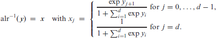
An important property of CoDa is given by the fact that the $(d+1)$ -part simplex $\mathbb{S}$ can be mapped bijectively onto a $d$ -dimensional Euclidean space of real vectors, such that approaches for the analysis and modelling of real-valued vectors are transferred to corresponding CoDa counterparts. The most simple among the common transformations is the additive-log-ratio transform, alr : $\mathbb{S}\to {\mathbb{R}}^d$ (Aitchison, 1986), which requires to first choose a divisor, the ‘ratioing variable’ (Filzmoser et al., 2018, p. 44). In common CoDa applications, however, where the categories in $\mathcal{S}$ are nominal, any such choice is arbitrary (Pawlowsky-Glahn and Buccianti, 2011, p. 5). In the case of ordinal CoDa, however, it appears reasonable to either take the highest category $s_d$ or lowest category $s_0$ for ‘ratioing’. To summarize an ordinal distribution, it is common to consider the cumulative distribution function $\left(\mathrm{C}\mathrm{D}\mathrm{F}\right)$ as it preserves the natural order, see the details in Section 3.1 below. Here, the probability $P\left(Q\le s_d\right)=1$ and is, thus, not informative, so one usually substitutes the highest category $s_d$ by all remaining categories $s_0,\dots ,s_{d-1}$ . For this reason, we shall also always use $s_d$ for ratioing the ordinal $\mathrm{C}\mathrm{o}\mathrm{D}\mathrm{a}$ , that is, we uniquely define

$\text{alr}\left(x\right)=y\text{with}{y}_{j+1}=\ln \left(\frac{x_j}{x_d}\right)\text{for}j=0,\dots ,d-1.$

(2.1)

The inverse of alr, the additive logistic transform, has the expression

${\text{alr}}^{-1}\left(y\right)=x\text{with}{x}_j=\left\{\begin{array}{l}\frac{\exp y_{j+1}}{1+{{\displaystyle \sum }}_{i=1}^d\exp y_i}\text{for}j=0,\dots ,d-1,\hfill \\ \frac{1}{1+{{\displaystyle \sum }}_{i=1}^d\exp y_i}\text{for}j=d.\hfill \end{array}\right.$

(2.2)

This backward transformation is also well-known in categorical data analysis, because it is the multinomial logit being commonly used for nominal regression and time series models (Agresti, 2002; Fokianos and Kedem, 2003).

Remark 1. While alr is attractive in view of the aforementioned connection to categorical data as well as the simplicity of (2.1)-(2.2), it has also been critized as it is not isometric and leads to disparate differences between the transformed points if using different ratioing variables (Pawlowsky-Glahn and Buccianti, 2011, p. 5). If isometry is crucial for applications, then one better uses an isometric log-ratio (ilr) transform (see Egozcue et al., 2003), such as the one defined by (5.5) later in Section 5.2. Also for ilr, it is possible to emphasize the role of $s_d$ by assigning it as the ‘pivot coordinate’, see Filzmoser et al. (2018, Section 3.3.3). On the other hand, the definition of ilr and its inverse are more complex than (2.1)-(2.2), and alr and ilr differ only by a linear transformation anyway (Egozcue et al., 2003, p. 298). Thus, we shall mainly focus on the alr in the following, but we also account for ilr at appropriate places.

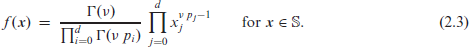
In this research, we are not only concerned with the descriptive analysis of ordinal CoDa, but approaches for statistical inference are considered as well, see Sections 4-6. For this reason, let us now turn to compositional RVs $\mathit{X}$ with range $\mathbb{S}$ (random compositions), where several parametric distributions are available in the literature. The probably most well-known model is the Dirichlet distribution, see Chapter 49 in Kotz et al. (2000) and Chapter 2 in Ng et al. (2011) for comprehensive surveys. $\mathrm{D}\mathrm{i}\mathrm{r}(\mathit{p},v)$ depends on a mean vector $\mathit{p}\in \mathbb{S}$ and a scale parameter $v\in (0;\mathrm{\infty })$ , and $\mathit{X}\sim \mathrm{D}\mathrm{i}\mathrm{r}(\mathit{p},v)$ is defined by the density function

$f\left(\mathit{x}\right)=\frac{\mathrm{\Gamma }\left(v\right)}{\prod _{i=0}^d\mathrm{\Gamma }\left(v{p}_i\right)}\prod _{j=0}^d{x}_j^v{p}_j-1\left(\mathrm{ }\right)\mathrm{f}\mathrm{o}\mathrm{r}\mathit{x}\in \mathbb{S}.$

(2.3)

The first- and second-order moments, for $i\ne j\in \{0,\dots ,d\}$ , are given by

$E\left[X_j\right]=p_j,V\left[X_j\right]=\frac{p_j\left(1-p_j\right)}{1+v},\text{Cov}\left[X_i,X_j\right]=\frac{-p_i{p}_j}{1+v}.$

(2.4)

The last formula implies that the Dirichlet distribution is only applicable if all cross-covariances of $\mathit{X}$ are negative, which is a strong limitation for practice (see Aitchison, 1986, p. 59). Therefore, the logistic normal distribution (Aitchison, 1986, Chapter 6) might be an attratcive competitor model for $\mathit{X}$ . We say that $\mathit{X}\sim \mathrm{L}\mathrm{N}(\mathit{\mu },\mathbf{\Sigma })$ if $\mathrm{a}\mathrm{l}\mathrm{r}\left(\mathit{X}\right)$ is normally distributed according to $\mathrm{N}(\mathit{\mu },\mathbf{\Sigma })$ , with $\mathit{\mu }\in$ ${\mathbb{R}}^d$ and positive definite $\mathrm{\Sigma }\in {\mathbb{R}}^{d\times d}$ . While, by contrast to (2.4), closed formulae for the marginal moments of $\mathit{X}\sim \mathrm{L}\mathrm{N}(\mathit{\mu },\mathbf{\Sigma })$ do not exist, some ratio moments are provided by Aitchison (1986, p. 116), and the ‘compositional mean’ ${\mathrm{a}\mathrm{l}\mathrm{r}}^{-1}\left(\mathit{\mu }\right)$ provides the component-wise medians of $\mathit{X}$ (Billheimer et al., 2001, p. 1208). Note that a CoDa-normal distribution might also be defined with respect to the ilr (as later done in Section 5.2). But as ilr and alr are linearly related to each other (recall Remark 1), a normally distributed $\mathrm{a}\mathrm{l}\mathrm{r}\left(\mathit{X}\right)$ implies a normal distribution for $\mathrm{i}\mathrm{l}\mathrm{r}\left(\mathit{X}\right)$ as well, and vice versa.

3 Applying ordinal statistics to CoDa

As outlined in Section 1, it shall be demonstrated for various application areas that we may gain additional insights into ordinal $\mathrm{C}\mathrm{o}\mathrm{D}\mathrm{a}$ if the existing CoDa approaches are complemented by methods derived from ordinal data analysis. Therefore, Section 3.1 starts with a brief survey on ordinal approaches, while Section 3.2 already presents their first application, namely to a descriptive analysis of ordinal CoDa.

3.1 Properties of ordinal distributions

Let $Q$ be an ordinal RV with range $\mathcal{S}$ and PMF $\mathit{p}\in \mathbb{S}$ . To account for the natural order among the categories, one commonly does not focus on Q’s PMF but on its CDF, which can be summarized in the $d$ -dimensional vector $\mathit{f}={\left(f_0,\dots ,f_{d-1}\right)}^{\mathrm{\top }}\in [0;1{]}^d$ . Here, we define $f_j=P\left(Q\le s_j\right)$ for $=$ $0,\dots ,d$ , where $f_d$ is omitted in $\mathit{f}$ as it necessarily equals one. For this reason, we also used the largest category $s_d$ for ratioing in (2.1) when defining the alr transform.

Remark 2. A popular approach for a parametric modelling of ordinal data is the latent-variable approach (Agresti, 2010, p. 11). If $\mathit{f}$ is a $d$ -dimensional CDF vector, and if $L$ is a (latent) realvalued $\mathrm{R}\mathrm{V}$ with specified $\mathrm{C}\mathrm{D}\mathrm{F}{F}_L\left(x\right)$ , then one represents $f$ by selecting the threshold parameters $-\mathrm{\infty }<{\eta }_0<\dots <{\eta }_{d-1}<+\mathrm{\infty }$ such that

$f_j=F_L\left({\eta }_j\right)\text{for }j=0,\dots ,d-1$

(3.1)

holds. In a sense, $\mathit{f}$ is reparametrized in terms of $\mathit{\eta }={\left({\eta }_0,\dots ,{\eta }_{d-1}\right)}^{\mathrm{\top }}$ . The most popular choice for $F_L$ is the (standard) logistic distribution, $L\sim \mathrm{L}\left(\mathrm{0,1}\right)$ , leading to the cumulative logit model. Here, $\mathrm{L}(\alpha ,\beta )$ denotes the logistic distribution with location parameter $\alpha$ and scale parameter $\beta$ (see Johnson et al., 1995, Chapter 23), which is defined by the CDF

$F_{\alpha ,\beta }\left(x\right)={\left[1+\text{exp}\left(-\frac{x-\alpha }{\beta }\right)\right]}^{-1}\text{for }x\in ℝ.$

(3.2)

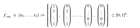
The CDF $\mathit{f}$ can be used to compute important stochastic properties of $Q$ . The location of $Q$ is commonly expressed in terms of the median (as this uses the order information), but also the mode (which is already well-defined for a nominal scale) might be used. Both median and mode take values in $\mathcal{S}$ , where the mode does not need to be unique. As $\mathcal{S}$ is typically of small size, the location measures provide only roughly graduated information about $Q$ . Much more measures are available to quantify the dispersion of $Q$ , see Blair and Lacy (1996), Kiesl (2003), Kvålseth (2011), Klein et al. (2016), Weiß 2019, 2022) for approaches and references. These measures are defined with respect to two extreme cases. Minimal dispersion happens if we are concerned with a one-point distribution on $\mathcal{S}$ , that is, if all probability mass concentrates in one category (maximal consensus):

${\mathit{f}}_{\mathrm{o}\mathrm{n}\mathrm{e}\mathrm{ }}\in \left\{{\mathit{t}}_0,\dots ,{\mathit{t}}_d\right\}:=\left\{\left(\begin{array}{c}1\\ 1\\ ⋮\\ 1\end{array}\right),\left(\begin{array}{c}0\\ 1\\ ⋮\\ 1\end{array}\right),\dots ,\left(\begin{array}{c}0\\ ⋮\\ 0\\ 1\end{array}\right),\left(\begin{array}{c}0\\ ⋮\\ 0\\ 0\end{array}\right)\right\}\subset [0;1{]}^{\mathrm{d.}}$

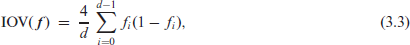
By contrast, $Q$ exhibits maximal dispersion if it follows the extreme two-point distribution (polarized distribution), $f_{\mathrm{t}\mathrm{w}\mathrm{o}}={\left(\frac{1}{2},\dots ,\frac{1}{2}\right)}^{\mathrm{\top }}$ , that is, if we have $50\mathrm{\%}$ probability mass in each of the outermost categories (maximal dissent). Note that the latter extreme differs from maximal nominal dispersion, which manifests itself in terms of a uniform distribution (maximal uncertainty). Ordinal dispersion measures are typically normalized to the range $[0;1]$ , and they take the value 0 (1) iff $Q$ exhibits minimal (maximal) dispersion. A few examples (see the above references for many further options) are the index of ordinal variation,

$\mathrm{I}\mathrm{O}\mathrm{V}\left(\mathit{f}\right)=\frac{4}{d}\sum _{i=0}^{d-1}{f}_i\left(1-f_{\mathrm{i,}}\right)$

(3.3)

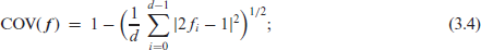
the coefficient of ordinal variation,

$\mathrm{cov}\left(\mathit{f}\right)=1-{\left(\frac{1}{d}\sum _{i=0}^{d-1}{\left|2f_i-1\right|}^2\right)}^{\frac{1}{2}};$

(3.4)

and the cumulative paired entropy (using the convention $0\cdot \mathrm{l}\mathrm{n}0=0$ ),

$\mathrm{C}\mathrm{P}\mathrm{E}\left(\mathit{f}\right)=\frac{-1}{d\mathrm{l}\mathrm{n}2}\sum _{i=0}^{d-1}\left(f_i\mathrm{l}\mathrm{n}{f}_i+\left(1-f_i\right)\mathrm{l}\mathrm{n}\left(1-f_{\mathrm{i.}}\right)\right)$

(3.5)

Finally, the (a)symmetry of $Q$ ’s distribution can be evaluated by measures of ordinal skewness, see Klein and Doll (2021), Weiß (2020) for details. We speak of symmetry if $p_i=p_{d-i}$ for all $i=0,\dots ,d$ , or equivalently, if $f_i=1-f_{d-1-i}$ for $i=0,\dots ,d-1$ . By contrast, maximal positive (negative) skewness is present if $p_0=1\left(p_d=1\right)$ , that is, the extreme left (right) one-point distribution. This corresponds to the CDFs $\mathit{f}=1={\mathit{t}}_0$ or $\mathit{f}=0={\mathit{t}}_d$ , respectively, where $1\left(0\right)$ denotes the vector of ones (zeros). These definitions of extreme skewness go along with the well-known rule of thumb that a positively skewed (= right-skewed) distribution appears to be left-leaning, and vice versa. A simple example of a normalized ordinal skewness measure is

$\text{skew}\left(f\right)=\frac{2}{d}{\displaystyle \sum }_{i=0}^{d-1}{f}_i-1\text{with range }\left[-1;1\right],$

(3.6)

Figure 1

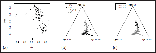
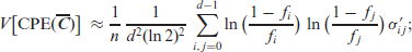
Age proportions in 195 countries from Example 1: plot of skew against IOV in (a), ternary diagrams in (b) and (c).

where skew $=+1(-1)$ for maximal positive (negative) skewness, and where skew $=0$ for a symmetric distribution.

3.2 Properties of ordinal CoDa

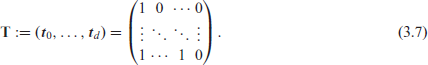
To apply the ordinal measures of Section 3.1 to ordinal CoDa $\mathit{x}\in \mathbb{S}$ , we have to accumulate these vectors first, that is, to compute $c:=\mathbf{T}\mathit{x}$ with the matrix

$\mathbf{T}:=\left({\mathit{t}}_0,\dots ,{\mathit{t}}_d\right)=\left(\begin{array}{cccc}1& 0& \cdots & 0\\ ⋮& \ddots & \ddots & ⋮\\ 1& \cdots & 1& 0\end{array}.\right)$

(3.7)

Then, we can evaluate the ordinal dispersion and skewness of $\mathit{x}$ by applying formulae (3.3)-(3.6) to $\mathit{c}$ instead of $\mathit{f}$ . Let us illustrate this approach and its benefits by two real-world data examples.

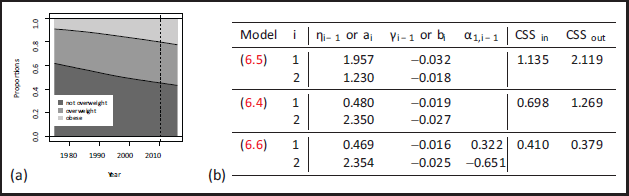
Example 1. The dataset ageCat World from the R-package robCompositions contains the proportions ${\mathit{x}}_i={\left(x_{i,0},x_{i,1},x_{i,2}\right)}^{\top },i=1,\dots ,n$ , of people with age $<15\left(x_{i,0}\right),15-60\left(x_{i,1}\right)$ , and $>60\left(x_{i,2}\right)$ in $n=$ 195 countries. These 3-part compositions refer to ordered categories, recall Section 1, thus constituting an example of ordinal CoDa. Since the dimension of the ${\mathit{x}}_i$ is three, a visual representation of the data by a ternary diagram is possible, see Figure 1. This shall help us to get an intuitive understanding of the ordinal measure (3.3)-(3.6) if being applied to the vectors ${\mathit{c}}_i:=\mathit{T}{\mathit{x}}_i$ .

As indicated in Section 3.1, the location measures do not provide much discriminative power: in 191 out of 195 cases, the median category is $s_1$ (‘age 15-60’), and $s_1$ is also the mode category for 163 of the ${\mathit{x}}_i$ . Next, let us turn to ordinal dispersion. Here, we solely focus on the $IOV\left({\mathit{c}}_i\right)$ values, as the IOV is most popular among practitioners, and as $COV\left({\mathit{c}}_i\right)$ and $CPE\left({\mathit{c}}_i\right)$ provide essentially equivalent insights in the present example, in the sense of strong positive correlation to $IOV\left(c_i\right)$ , being $>0.99$ in both cases (also see the discussion in Supplement S.1). As can be seen from Figure 1 (a), the values of $IOV\left({\mathit{c}}_i\right)$ vary between 0.4 and 0.8, that is, we are concerned with medium to strong dispersion. In fact, only few countries lead to an IOV less than 0.6. These information are related to a ternary diagram of the data in Figure 1 (a). The few countries with IOV less than 0.6 (shown as empty circles) are those with a high proportion of people with age 15-60, that is, these compositions are quite close to a onepoint distribution (the three possible one-point distributions correspond to the corners of the triangle). Countries having an IOV $\ge 0.7$ , in turn, are plotted (by grey dots) relatively close to the axis between the lowest and largest age category, that is, the outermost categories are more dominant.

Next, we consider the $skew\left({\mathit{c}}_i\right)$ values. Figure 1 (a) shows that we have at most moderate skewness values, with maximal absolute extent around 0.4, where positive skewness values are slightly more frequent than negative ones. Note that countries with negative skewness tend to show larger dispersion than in the case of positive skewness. The ternary diagram in Figure 1 (c) shows that positive skewness values refer to the lower-left half of the triangle, which is easy to interpret: right-skewed compositions are left leaning, so the lower categories dominate the upper ones.

Example 1 showed that for ordinal 3-part compositions, the IOV-skew diagram provides similar insights into the data as the ternary diagram. However, an IOV-skew diagram can also be drawn for higher-dimensional compositions, whereas a ternary diagram is not immediately applicable (one could combine individual categories into larger ones before plotting). By contrast, the IOV-skew diagram allows to directly visualize the high-dimensional ordinal compositions, being easy to interpret by a practitioner, see the data example in Supplement S.1. To sum up, Section 3 demonstrated that ordinal measures such as IOV and skew, if applied to ordinal CoDa, provide new insights into the data (which may also be presented visually) and, thus, constitute a valuable complement to existing methods for descriptive CoDa analysis.

4 Statistical inference for ordinal CoDa

In Section 3.2, we applied the proposed statistics for ordinal $\mathrm{C}\mathrm{o}\mathrm{D}\mathrm{a}$ in a descriptive way. To be able to compute confidence regions or to test for significant differences, we shall now consider the distributional properties of such statistics. In Section 4.1, we derive their asymptotic distribution and investigate the corresponding finite-sample performance. A further real-world data example is discussed in Section 4.2.

4.1 Asymptotic distributions and simulation results

Let ${\mathit{X}}_1,\dots ,{\mathit{X}}_n$ be an independent and identically distributed (i.i. d.) sample of ordinal compositional RVs with mean $\mathit{p}$ , let $\bar{X}$ denote their sample mean. Then, the central limit theorem (CLT) implies that $\sqrt{n}(\stackrel{-}{\mathit{X}}-\mathit{p})$ is asymptotically normally distributed (see Serfling, 1980), namely

$\sqrt{n}\left(\bar{X}-p\right)\sim \text{N}\left(0,\Sigma \right)\text{with}\Sigma ={\left({\sigma }_{ij}\right)}_{i,j=0,\dots ,d}\text{ and }{\sigma }_{ij}=\text{Cov}\left[X_i,X_{j.}\right]$

(4.1)

While (4.1) holds for nominal CoDa as well, we now turn to the accumulated versions of $\mathit{X}$ and $\mathit{p}$ , that is, to ${\mathit{C}}_k=\mathbf{T}{\mathit{X}}_k$ for $k=1,\dots ,n$ with mean $E\left[{\mathit{C}}_k\right]=\mathit{f}=\mathbf{T}\mathit{p}$ , where $\mathbf{T}$ is the transformation matrix from (3.7). These are meaningful only for ordinal CoDa, and they are required for the computation of the ordinal statistics (3.3)-(3.6). The asymptotics of the sample mean $\stackrel{-}{\mathit{C}}$ follow immediately from (4.1) and the linearity properties of the multivariate normal distribution, namely

$\sqrt{n}(\stackrel{-}{\mathit{C}}-\mathit{f})\sim \mathrm{N}\left(0,{\mathbf{\Sigma }}^{\mathrm{\text{'}}}\right)\mathrm{w}\mathrm{i}\mathrm{t}\mathrm{h}{\mathbf{\Sigma }}^{\mathrm{\text{'}}}=\mathbf{T}\mathbf{\Sigma }{\mathbf{T}}^{\mathrm{\top }}.$

(4.2)

The entries of ${\mathbf{\Sigma }}^{\mathrm{\text{'}}}$ are computed as

$${\sigma }_{ij}^{\prime }=T_{i•}\Sigma T_{j•}^{\top }={\displaystyle {\sum }_{r=0}^i{\displaystyle {\sum }_{s=0}^j{\sigma }_{rs}}}\text{for}i,j=0,\dots ,d-1,$$

where ${\mathbf{T}}_{k⦁}$ abbreviates the $k$ th row vector of $\mathbf{T}$ . Finally, the asymptotics of the ordinal statistics (3.3)(3.6), if applied to the estimator $\overline{C}$ , are derived based on Taylor expansions (‘Delta method’), see Supplement S.2 for details. The obtained results are summarized in the following theorem.

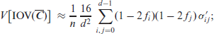
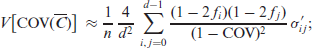
Theorem 1. Let $\overline{C}$ be computed from an i.i.d. ordinal CoDa sample, let the ${\sigma }_{ij}^{\prime }$ be given as in (4.2). Then, the ordinal measures (3.3)-(3.6) are asymptotically normally distributed with asymptotic variances

$$V[\text{IOV}(\overline{C})]\approx \frac{1}{n}\frac{16}{d^2}\sum _{i,j=0}^{d-1}\left(1-2f_i\right)\left(1-2f_j\right){\sigma }_{ij}^{\prime }$$

$$V[\text{COV}(\overline{C})]\approx \frac{1}{n}\frac{4}{d^2}{\displaystyle \sum }_{i,j=0}^{d-1}\frac{\left(1-2f_i\right)\left(1-2f_j\right)}{{(1-\text{COV})}^2}{\sigma }_{ij}^{\prime };$$

$$V[\text{CPE}(\overline{C})]\approx \frac{1}{n}\frac{1}{d^2{(\ln 2)}^2}{\displaystyle \sum }_{i,j=0}^{d-1}\ln \left(\frac{1-f_i}{f_i}\right)\ln \left(\frac{1-f_j}{f_j}\right){\sigma }_{ij}^{\prime };$$

$$V[\text{skew}(\overline{C})]\approx \frac{1}{n}\frac{4}{d^2}{\displaystyle \sum }_{i,j=0}^{d-1}{\sigma }_{ij}^{\prime }.$$

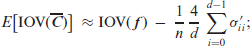
While $E\left[\mathrm{s}\mathrm{k}\mathrm{e}\mathrm{w}\right(\stackrel{-}{\mathit{C}}\left)\right]=\mathrm{s}\mathrm{k}\mathrm{e}\mathrm{w}\left(\mathit{f}\right)$ holds exactly, the means of the remaining measures are approximately equal to

$$E[\text{IOV}(\overline{C})]\approx \text{IOV}(f)-\frac{1}{n}\frac{4}{d}{\displaystyle \sum }_{i=0}^{d-1}{\sigma }_{ii}^{\prime };$$

$$E[\text{COV}(\overline{C})]\approx \text{COV}(f)+\frac{1}{n}\frac{2}{d}{\displaystyle \sum }_{i,j=0}^{d-1}\left(\frac{\left(1-2f_i\right)\left(1-2f_j\right)}{d{(1-\text{COV})}^3}-\frac{{\delta }_{ij}}{1-COV}\right){\sigma }_{ij}^{\prime };$$

$$E[\text{CPE}(\overline{C})]\approx \text{CPE}(f)-\frac{1}{n}\frac{1}{2d\ln 2}{\displaystyle \sum }_{i=0}^{d-1}\frac{1}{f_i\left(1-f_i\right)}{\sigma }_{ii}^{\prime }.$$

Figure 2

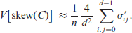
Proportions of education levels in 31 European countries from Section 4.2: ternary diagram in (a), plot of skew against IOV in (b), estimates in (c).

For the practical implementation of the asymptotics, it is suggested to compute the ${\sigma }_{ij}^{\text{'}}$ separately, and to plug-in the results into the formulae of Theorem 1. In the special case of a Dirichlet distribution, see Example 1 in Supplement S.2, closed-form formulae for the ${\sigma }_{ij}^{\text{'}}$ exist such that further simplifications are possible.

In practice, the asymptotic distributions of Theorem 1 are used to approximate the true distributions of the ordinal statistics $\text{IOV}\left(\overline{C}\right),\dots ,\text{skew}\left(\overline{C}\right)$ according to (3.3)-(3.6). Therefore, it is important to check the approximation quality of these distributions for finite sample sizes $n$ . For this purpose, the simulation study summarized in Supplement S.3 was done, where i. i. d. ordinal CoDa samples according to a $\text{Dir}\left(p,v\right)$ -distribution and a $\text{LN}\left(\mu ,\Sigma \right)$ -distribution were simulated (with ${10}^6$ replications per scenario). The actual parametrization of these distributions is inspired by the subsequent data example in Section 4.2. Details on the simulation procedures as well as on required numerical approaches for the LN-case are discussed in Supplement S.3. It turns out that we generally have an excellent agreement between simulated and asymptotic properties. Thus, the bias and SD being observed in finite samples are well described by the asymptotics of Theorem 1 .

4.2 Illustrative data example

We analyse the dataset educFM in the R-package robCompositions (also see Filzmoser et al., 2018, Section 10.7.3), which provides the proportions of low, medium, and high education levels of father and mother in $n=31$ European countries. So for each country $i\in \left\{1,\dots ,n\right\}$ , two 3-part compositions are available, say $x_{\text{f},i}$ and $x_{\text{m};i}$ for father and mother, respectively. The category $s_0$ (‘low’) is the median (mode) of $x_{\text{f};i}$ in 19 (22) cases, and the median (mode) of $x_{\text{m};i}$ in 22 (25) cases; otherwise, it is the category $s_1$ (‘medium’). The ternary plot in Figure 2 (a) shows that the CoDa concentrate in the low-to-medium corner, which goes along with the positive skew $\left(c_{\text{*};i}\right)$ values in part (b), implying left-leaning distributions. The $\text{IOV}\left(c_{\text{*};i}\right)$ values cover a wide range from low to high dispersion. It also interesting to note the pronounced structure in the IOV-skew diagram, where low dispersion is connected to strong positive skewness, that is, the corresponding CoDa vectors are close to a one-point distribution in the lowest category.

Next, we analyse if there are significant differences (on a 5%-level) between the education proportions of father and mother; from the plots in Figure 2 (black vs. grey dots), no such difference can be recognized. For this purpose, models for both datasets are required. A natural first idea is to try a Dirichlet distribution, but a problem becomes clear: the sample covariance matrices for the fathers’ and mothers’ compositions are $\left(\begin{array}{ccc}0.036& -0.027& -0.009\\ -0.027& 0.022& 0.005\\ -0.009& 0.005& 0.005\end{array}\right)$ and $\left(\begin{array}{ccc}0.029& -0.022& -0.007\\ -0.022& 0.019& 0.003\\ -0.007& 0.003& 0.004\end{array}\right)$ , respectively, that is, some cross-covariances are positive, which is not consistent with a Dirichlet distribution, recall (2.4). Thus, logistic normal distributions seem more appropriate, as also confirmed by the distributional analyses presented in Supplement S.4. Thus, the following discussion focusses on the LN model (fitted by mvnorm.mle in the R-package Rfast), whereas results regarding the Dirichlet model are presented in Supplement S.4.

The fitted $\text{LN}\left(\mu ,\Sigma \right)$ -models are ${\mu }_{\text{f}}={(1.451,0.797)}^{\top },{\Sigma }_{\text{f}}=\left(\begin{array}{ll}0.721\hfill & 0.028\hfill \\ 0.028\hfill & 0.278\hfill \end{array}\right)$ and ${\mu }_{\text{m}}=$ ${(1.969,1.084)}^{\top },{\Sigma }_{\text{m}}=\left(\begin{array}{ll}0.728\hfill & 0.171\hfill \\ 0.171\hfill & 0.418\hfill \end{array}\right)$ , respectively, which both lead to a rather good fit to the CoDa's means and cross-covariances. Hence, the LN-models are used as the base for asymptotic computations. The point estimates from $\text{IOV}\left(\overline{C}\right)$ and skew $\left(\overline{C}\right)$ , as well as the corresponding asymptotic biases and standard errors (SEs) according to Theorem 1, are shown in Figure 2 (c). The biases of $\text{IOV}\left(\overline{C}\right)$ are negligible relative to the actual estimates, and skew is unbiased anyway. Comparing the IOV and skew estimates between father and mother, we recognize a notable difference, which is larger than twice a standard error. So in view of the estimators’ asymptotic normality, we conclude that the IOV and skew estimates are significantly different between father and mother. In fact, we have less dispersion and stronger positive skewness for mothers, that is, the mothers’ education proportions are (in the mean) closer to a one-point distribution in the category ‘low’. This might be interpreted as an indication of unequal opportunities for education among males and females in the past.

5 Monitoring ordinal CoDa

In applications related to manufacturing industries or health surveillance, one commonly monitors an ongoing process of certain quality characteristics for the possible occurrence of a process change. The main tool for such an online monitoring are control charts, see Montgomery (2009) for detailed information. Control charts are designed with respect to a specified in-control model, that is, when the process runs in a stable state. If the process’ distribution changes at a certain time point $\tau \in \mathbb{N}$ (out-of-control situation), then $\tau$ is said to be a change point, and the aim is to detect this process change as soon as possible. More precisely, the in-control distribution of the process is used to compute so-called control limits (CLs), and the incoming process observations (or statistics computed thereof) are sequentially plotted on a chart being equipped with these CLs. If a plotted statistic violates the CLs, then an alarm is triggered at this time to indicate that the process might have run out of control (the time until the first alarm (stopping time) is called the run length of the control chart). An alarm under in-control (out-of-control) conditions is classified as a false (true) alarm. To evaluate the performance of a control chart, one computes the mean of the run length (average run length, ARL), that is, the mean number of plotted statistics from the beginning of process monitoring until the first false alarm. The in-control ARL should be sufficiently large for practice to avoid too frequent false alarms. An out-of-control ARL, by contrast, expresses the mean delay from the change point to the true alarm, and this number should be as small as possible. For chart design, one first specifies a target value for the in-control ARL, say $AR{L}_0$ , then one computes the CLs such that ${\text{ARL}}_0$ is met at least in good approximation.

5.1 Control charts for ordinal CoDa

In what follows, we are concerned with the monitoring of an ordinal CoDa process ${\left(X_t\right)}_{t\in \mathbb{N}}$ , which is assumed to be i. i. d. in time $t$ under in-control conditions. There are several proposals for CoDa control charts in general (i. e., nominal CoDa), see Holmes and Mergen (1993), Vives-Mestres et al. 2013, 2014 and references therein, but none for the particular case of ordinal CoDa. In fact, the data application (manufacturing of grit) considered in the aforementioned articles exhibits ordered categories, because it refers to the particle size proportions with categories ‘large’, ‘medium’, and ‘small’; see Table 2 in Holmes and Mergen (1993) for a sequence of 56 CoDa vectors. This ordinal information, however, was not used for defining the control charts. Instead, Holmes and Mergen (1993), Vives-Mestres et al. 2013, 2014 used types of Hotelling- $T^2$ chart (see Montgomery, 2009, Section 11.3), which apply to unordered categories as well: while Holmes and Mergen (1993) computed the $T^2$ statistic based on two of the three components of $X_t$ , Vives-Mestres et al. (2013, 2014) first mapped the 3-part simplex $\mathbb{S}$ onto ${ℝ}^2$ and then computed the $T^2$ -statistic. Generally, see Section 11.3 in Montgomery (2009), if $\left(Y_t\right)$ is a multivariate vector-valued process with in-control mean ${\mu }_0$ and covariance matrix ${\Sigma }_0$ , the ${\chi }^2$ -chart is defined by plotting the statistics

${\text{X}}_t^2={\left(Y_t-{\mu }_0\right)}^{\top }{\Sigma }_0^{-1}\left(Y_t-{\mu }_0\right)\text{ for }t=1,2,\dots$

(5.1)

against an upper CL (UCL) chosen such that the ${\text{ARL}}_0$ -target is met, that is, an alarm is triggered if ${\text{X}}_t^2>\text{UCL}$ . The Hotelling- $T^2$ chart differs from (5.1) by using estimates for ${\mu }_0$ and ${\Sigma }_0$ instead (and by adapting the UCL appropriately). Besides not using the ordinal information, statistic (5.1) has the drawback that an alarm is difficult to interpret (see Montgomery, 2009, p. 505), because the value of ${\text{X}}_t^2$ does indicate the actual type of out-of-control situation; see Vives-Mestres et al. (2013) for a discussion. Thus, if monitoring ordinal CoDa, it is suggested to complement the CoDa ${\chi }^2$ - or $T^2$ -chart by further control charts based on the ordinal statistics in Section 3.1, such that a targeted diagnosis of the actual out-of-control state is possible.

To monitor the process $\left(X_t\right)$ or $\left(C_t\right)$ , respectively, two types of IOV-chart are developed by adapting the corresponding proposals in Ottenstreuer et al. (2023). Let $p_0$ and $f_0$ denote the in-control means of $\left(X_t\right)$ and $\left(C_t\right)$ , respectively. We shall consider two-sided chart designs, that is, with both a lower and upper CL (LCL and UCL, respectively). Then, the Shewhart IOV-chart is defined by plotting

$\text{IOV}\left(C_t\right)\text{ for }t=1,2,\dots$

(5.2)

against LCL and UCL, which are chosen such that the in-control ARL is close to $AR{L}_0$ . An alarm is triggered if either $\text{IOV}\left(C_t\right)<\text{LCL}$ or $\text{IOV}\left(C_t\right)>\text{UCL}$ . As this decision relies solely on the $t^{\text{th }}$ observation $C_t$ , Shewhart-type charts typically react quickly to very large process shifts, but rather slow to small process changes.

To equip the IOV-chart with an additional memory and to, thus, improve the sensitivity towards small process changes, we also consider an exponentially weighted moving-average (EWMA) approach in analogy to Ottenstreuer et al. (2023). For the smoothing parameter $\lambda \in \left(0;1\right)$ , we recursively compute $C_{t,\lambda }=\lambda C_t+\left(1-\lambda \right)C_{t-1,\lambda }$ with $C_{0,\lambda }=f_0$ . Then, the EWMA IOV-chart is defined by plotting

$\text{IOV}\left(C_{t,\lambda }\right)\text{ for }t=1,2,\dots$

(5.3)

against appropriately chosen LCL, UCL. Note that $\lambda \to 1$ leads to the Shewhart chart (5.2), whereas decreasing values of $\lambda$ increase the inherent memory of (5.3).

Both IOV-charts (5.2) and (5.3) are defined to detect changes in the ordinal dispersion. A violation of LCL (UCL) indicates a decrease (increase) of dispersion and, thus, allows for a targeted diagnosis. Instead of the IOV (3.3), one could also use the COV (3.4) or CPE (3.5), but we focus on the IOV for convenience. However, it seems reasonable to also consider the Shewhart and EWMA version of a skew chart based on (3.6), as such a chart could react to changes in ordinal skewness, see Ottenstreuer et al. (2023). Hence, we also plot

$\text{skew}\left(C_{t,\lambda }\right)\text{ for }t=1,2,\dots$

(5.4)

against appropriate $\text{LCL},\text{UCL}$ , where $\lambda =1$ corresponds to the Shewhart skew-chart, and $\lambda \in \left(0;1\right)$ to the EWMA skew-chart. To sum up, at least theoretically, the IOV- and skew-charts offer the potential for a targeted diagnosis of the actual out-of-control scenario. In the subsequent Section 5.2, we provide empirical evidence that such targeted conclusions are indeed possible.

5.2 Empirical illustrations

As mentioned in Section 5.1, Vives-Mestres et al. 2013, 2014 applied a $T^2$ -type control chart to the CoDa process $\left(X_t\right)$ , namely after first mapping the 3-part simplex $\mathbb{S}$ onto ${ℝ}^2$ . A possible solution for this mapping could have been the alr transform $\left(2.1\right)$ , but Vives-Mestres et al. 2013, 2014 used types of ilr transforms instead. To make the subsequent results comparable to those in Vives-Mestres et al. (2014), in this section, we shall consider their specific ilr transform defined by

$\text{ilr}\left(x\right)=y\in {ℝ}^2\text{ with }{y}_1=\frac{1}{\sqrt{2}}\text{ln}\frac{x_1}{x_2},y_2=\sqrt{\frac{2}{3}}\text{ln}\frac{\sqrt{x_1{x}_2}}{x_0}.$

(5.5)

It should be noted, however, that because of the relation $\text{ln}\frac{\sqrt{x_1{x}_2}}{x_0}=\frac{1}{2}\text{ln}\frac{x_1}{x_2}-\text{ln}\frac{x_0}{x_2}$ , it holds that $\text{ilr}\left(x\right)=\left(\begin{array}{cc}0& 1/\sqrt{2}\\ -\sqrt{2/3}& 1/\sqrt{6}\end{array}\right)\text{alr}\left(x\right)$ , that is, ilr and alr only differ by a linear transformation, also recall Remark 1. We use the CoDa-normal distribution implied by requiring that $\text{ilr}\left(X\right)\sim \text{N}\left(\mu ,\Sigma \right)$ with $\mu \in {ℝ}^2$ and positive definite $\text{Σ}\in {ℝ}^{2\times 2}$ , also see Mateu-Figueras et al. (2013), which is a reparametrization of the LN-distribution discussed in Section 2. This distribution is relevant for chart design, as we have to specify the in-control model for the process $\left(X_t\right)$ . Like in Vives-Mestres et al. (2014), we define the in-control model as $\text{ilr}\left(X\right)\sim \text{N}\left({\mu }_0,{\Sigma }_0\right)$ with ${\mu }_0\approx {(1.959,1.158)}^{\top }$ and ${\text{Σ}}_0\approx \left(\begin{array}{cc}0.134& -0.032\\ -0.032& 0.097\end{array}\right)$ , which are the sample values from the ilr-transformed particles dataset $x_1,\dots ,x_{56}$ in Table 2 of Holmes and Mergen (1993). For comparability, we also use the same target $\text{ARL}$ , namely ${\text{ARL}}_0=333.\overline{3}$ . Note that the above ${\mu }_0$ corresponds to the component-wise means $p_0\approx {(0.057,0.881,0.062)}^{\top }$ (computed by numerical integration) and component-wise medians ilr^-1 $\left({\mu }_0\right)\approx {(0.054,0.890,0.056)}^{\top }$ for $X$ , that is, we have a nearly symmetric mean/median particle size proportion under in-control conditions, which also exhibits only low dispersion. More precisely, $\text{IOV}\left(p_0\right)\approx 0.223$ and $\text{skew}\left(p_0\right)\approx -0.005$ . Note that a monitoring of ordinal location would not be promising: because of the large mean/median proportion of category $s_1$ (‘medium’), we can hardly ever expect to observe any other median or mode category than $s_1$ . In fact, for the data in Table 2 of Holmes and Mergen (1993), $s_1$ is the median and mode category without exception.

The aforementioned in-control model is now used for chart design. For given values of the design parameters, ${10}^5$ in-control processes are simulated and the run lengths (i. e., the numbers of statistics until the first signal) are determined; the mean across these run lengths approximates the true ARL value. For chart design, the design parameters are varied (and ARL simulation is repeated for each revised design) until the ${\text{ARL}}_0$ -target is met in close approximation. In this way, we determine the chart design of the Shewhart and EWMA versions of IOV- and skew-chart (5.2)-(5.4), where the EWMA charts use $\lambda =0.1$ . As a competitor, we consider the Shewhart ${\chi }^2$ -chart (5.1) in analogy to Vives-Mestres et al. (2014). Furthermore, for the sake of completeness, we also consider the multivariate EWMA version of this chart defined like in Section 11.4 of Montgomery (2009):

${\text{X}}_{t,\lambda }^2=\frac{2-\lambda }{\lambda }{\left(1-{(1-\lambda )}^{2t}\right)}^{-1}{\left(Z_{t,\lambda }-{\mu }_0\right)}^{\top }{\Sigma }_0^{-1}\left(Z_{t,\lambda }-{\mu }_0\right)\text{ for }t=1,2,\dots ,$

(5.6)

where $Z_{t,\lambda }=\lambda Y_t+\left(1-\lambda \right)Z_{t-1,\lambda }$ with $Z_{0,\lambda }={\mu }_0$ . Although both EWMA charts (5.3) and (5.6) are not directly comparable because of a different implementation of the EWMA approach, we use again $\lambda =0.1$ for illustration. The resulting designs and in-control ARLs are summarized in the first block (italic font) of Table S.6.1 in Supplement S.6.

Next, these chart designs are used for a simulation-based analysis of the out-of-control performance. Based on an ordinal logit approach (recall Remark 2), we define several out-of-control scenarios for ilr^-1 (μ) (medians of CoDa distribution), see Supplement S.5 for details. The logit approach accounts for the order among the categories, and it allows to distinguish between dispersion and skewness shifts for ${\text{ilr}}^{-1}\left(\mu \right)$ compared to ${\text{ilr}}^{-1}\left({\mu }_0\right)$ . The simulation results discussed in Supplement S. 6 show that the IOV-, skew-, and ${\chi }^2$ -charts have a quite different out-of-control performance. While the ${\chi }^2$ -chart is universally applicable but does not allow to conclude from the signal on the type of out-of-control scenario, the IOV-and skew-charts are sensitive only to specific out-of-control scenarios, namely such affecting dispersion and skewness, respectively. Thus, running an IOV- and skew-chart in parallel to a ${\chi }^2$ -chart (preferably always the EWMA version), we can expect that a dispersion shift leads to an early alarm of the IOV-chart, and a skewness shift to one of the skew-chart. In this way, the types of alarm allow us to conclude on the type of out-of-control situation.

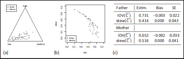
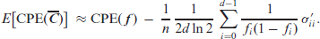
This type of diagnostic feature is illustrated by Figure 3, where the EWMA IOV-and skew-chart are applied to the particle size proportions of Table 2 in Holmes and Mergen (1993). The skewchart in (b) does not trigger any alarm during the monitoring period, so we have no indication of a systematic skewness change. The IOV-chart in (a), by contrast, triggers alarms at times $t=16,17$ as well as $t=23,24$ . In both cases, the LCL is violated, indicating that there was an exceptionally low dispersion for $t\le 16$ and $t\le 23$ . Further analysing the raw data, we indeed note that $x_{15}=$ $\left(0.026,0.945,0.029\right)$ and $x_{16}=\left(0.027,0.945,0.028\right)$ are considerably less dispersed than ${\text{ilr}}^{-1}\left({\mu }_0\right)\approx$ ${(0.054,0.890,0.056)}^{\top }$ (but still nearly symmetric). Note that $x_{15},x_{16}$ are close to the second scenario in the fifth block of Table S.6.1. Analogous results (though less pronounced) hold for observations $x_{21},\dots ,x_{24}$ . Finally, although it did not suffice for an alarm yet, we recognize increasing dispersion and skewness towards the end of the monitoring period in Figure 3.

Figure 3

Particle size proportions from Section 5.2: EWMA IOV-chart in (a) and EWMA skew-chart in (b), where $\lambda =0.1$ .

6 Ordinal compositional time series

Let $\mathbb{Z}=\left\{\dots ,-1,0,1,\dots \right\}$ . We refer to a stochastic process ${\left(X_t\right)}_{t\in \mathbb{Z}}$ , which consists of CoDa RVs, as a $\text{CoDa}$ processes. A compositional time series (CoTS) is a finite-length segment taken thereof.

6.1 Analysis and modelling of ordinal CoTS

Several models for CoDa processes $\left(X_t\right)$ and the resulting CoTS $X_1,\dots ,X_n$ have been proposed during the last years. The most common approach for modelling CoTS is to first map the $\left(d+1\right)$ part compositions $X_t$ onto $d$ -dimensional real vectors $Y_t$ (e. g., by taking the alr transform (2.1) or an ilr transform), and to then apply a vector autoregressive moving-average (VARMA) model to the transformed time series $\left(Y_t\right)$ , see, for example, Mills (2010), Dawson et al. (2014). Because of the large number of VARMA model parameters, for short time series, also simple regression approaches have been proposed, that is, the component series $\left(Y_{t,i}\right)$ of the transformed CoTS are considered as linear or quadratic regression models in time $t$ , see, for example, Wang et al. (2007), Mills (2010). A parsimonious ARMA-type model for CoTS relying on the use of a variation operator was proposed by Möller and Weiß (2020). Also Zheng and Chen (2017) proposed a class of ARMA-type models for CoTS, being based on a conditional regression approach. For references on further model types, see Pawlowsky-Glahn and Buccianti (2011, Chapter 7) and Zheng and Chen (2017).

All the aforementioned time series models are developed to deal with general (nominal) CoDa, that is, a possible order among the categories is not considered. However, several of the examples presented in the literature are ordinal CoTS. For example, Wang et al. (2007) discuss a time series of yearly proportions of employed persons in China, where the proportions refer to the three production sectors ‘primary industry’, ‘secondary industry’, and ‘tertiary industry’; also see Supplement S.7. Mills (2010) modelled obesity trends in England, expressed by yearly proportions of persons falling into ordered weight categories, ranging from ‘not overweight’ to ‘obese’; also see Section 6.2. As a last example, Dawson et al. (2014) analysed a time series expressing the attitude of UK people towards the Olympic Games, with ordered categories from ‘strongly against’ to ‘strongly supportive’. In any of these examples, it could be beneficial to explicitly account for the ordered categories while analysing the data, which is illustrated by the data example discussed in Supplement S.7.

Not only for their analysis, but also for the modelling of ordinal CoTS, it could be relevant to account for the ordered categories. As a possible solution, we combine the conditional regression model of Zheng and Chen (2017) with the cumulative logit approach of Remark 2, in analogy to the ordinal time series models of Pruscha (1993); Fokianos and Kedem (2003). Zheng and Chen (2017) propose a conditional modelling of $\left(X_t\right)$ . If ${\mathcal{F}}_s$ denotes the $\sigma$ -field generated by all information up to time $s$ , then $X_t\mid {\mathcal{F}}_{t-1}$ is assumed to follow a specified CoDa distribution with parameter vector ${\theta }_t$ , say $X_t\mid {\mathcal{F}}_{t-1}\sim \text{CoDa}\left({\theta }_t\right)$ , where ${\theta }_t$ is computed from the information up to time $t-1$ . For example, we would define ${\theta }_t={\left(p_{t,0},\dots ,p_{t,d-1},v\right)}^{\top }$ if $X_t$ is conditionally Dirichlet-distributed with time-invariant scale parameter $v$ , that is, $X_t\mid {\mathcal{F}}_{t-1}\sim \text{Dir}\left(p_t,v\right)$ according to (2.3), where $p_{t,d}=1-p_{t,0}-\dots -p_{t,d-1}$ . In this case, the conditional mean of $X_t$ equals $E\left[X_t\mid {\mathcal{F}}_{t-1}\right]=p_t$ , and the conditional (co)variances are adjusted by the factor $1/\left(1+v\right)$ , recall (2.4). As suggested by Zheng and Chen (2017), $p_t$ could be modelled by an ARMA-type recursion of the form $p_t=\varphi \left(X_{t-1},\dots ,X_{t-\text{p}},p_{t-1},\dots ,p_{t-\text{q}}\right)$ , where $\text{p}\in \mathbb{N}$ expresses the autoregressive order and $\text{q}\in {\mathbb{N}}_0=\left\{0,1,\dots \right\}$ the ‘moving-average’ order (it is more appropriate to interpret $p_{t-1},\dots ,p_{t-\text{q}}$ as forming a feedback term). Specific examples for choosing $\varphi$ in the case of nominal CoDa are discussed by Zheng and Chen (2017).

In what follows, to account for the natural order of ordinal $\text{CoDa}$ and to reduce the number of model parameters at the same time, we present possible specifications for $\varphi$ being derived from the cumulative logit approach, in analogy to Pruscha (1993); Fokianos and Kedem (2003). Define ${\tilde{X}}_t={\left(X_{t,0},\dots ,X_{t,d-1}\right)}^{\top }$ and ${\tilde{p}}_t={\left(p_{t,0},\dots ,p_{t,d-1}\right)}^{\top }$ , and let $f_t$ denote the corresponding $d$ -dimensional conditional CDF vector. Recall that $F_{0,1}$ denotes the CDF of the standard logistic distribution (inverse logit function). An ARMA-type model for ordinal CoTS is defined by the recursion

$f_{t,i}=F_{0,1}\left({\eta }_i+{\displaystyle {\sum }_{k=1}^{\text{p}}{\alpha }_k^{\top }{\tilde{X}}_{t-k}+{\displaystyle {\sum }_{l=1}^{\text{q}}{\beta }_l^{\top }{\tilde{p}}_{t-l}}}\right)\text{for}i=0,\dots ,d-1,$

(6.1)

which has the $d\left(\text{p}+\text{q}+1\right)$ parameters involved in $\eta ,{\alpha }_1,\dots ,{\alpha }_{\text{p}},{\beta }_1,\dots ,{\beta }_{\text{q}}$ . The parameters ${\alpha }_1,\dots ,{\beta }_{\text{q}}$ control the serial dependence structure, which is unique across the categories. The individual ordinal categories are accounted for by the parameter $\eta ={\left({\eta }_0,\dots ,{\eta }_{d-1}\right)}^{\top }$ with $-\infty <{\eta }_0<$ $\dots <{\eta }_{d-1}<+\infty$ . A more parsimonious model specification, also see Pruscha (1993), is

$f_{t,i}=F_{0,1}\left({\eta }_i+{\displaystyle {\sum }_{k=1}^{\text{p}}{\alpha }_k{1}^{\top }{\tilde{X}}_{t-k}+}{\displaystyle {\sum }_{l=1}^{\text{q}}{\beta }_l{1}^{\top }{\tilde{p}}_{t-l}}\right)\text{for}i=0,\dots ,d-1,$

(6.2)

which has only $d+\text{p}+\text{q}$ parameters. If the data are then generated according to $X_t\mid {\mathcal{F}}_{t-1}\sim$ $\text{Dir}\left(p_t,v\right)$ , for example (where $p_t$ follows from $f_t$ by taking discrete differences), we also have the additional scale parameter $v$ from the Dirichlet distribution. Models (6.1) and (6.2) are easily adapted to account for possible covariate information $z_t$ by adding the summand ‘ $+{\gamma }^{\top }{z}_t$ ’ within the parentheses.

Figure 4

Proportions of weight categories from Section 6.2: (a) plot of proportions over time, and (b) table with model fits and corresponding CSS values.

Parameter estimation can be done by a conditional least-squares (CLS) approach, that is, by numerically minimizing the conditional sum of squares (CSS) defined by

$\text{CSS}(\theta ):={\displaystyle \sum }_t\parallel X_t-p_t{\parallel }^2\to \min ,$

(6.3)

where $\theta$ comprises all parameters involved in (6.1) or (6.2), respectively, and where $\parallel \cdot \parallel$ denotes the Euclidean norm. The CLS approach is semi-parametric in the sense that it does not require to specify the full conditional distribution of $X_t\mid {\mathcal{F}}_{t-1}$ but only the equation for the conditional mean, which, in turn, is useful for predicting future $\text{CoDa}$ values. It is also easy to formulate a conditional log-likelihood approach for models (6.1) and (6.2), but this requires to fully specify the distribution of $X_t\mid {\mathcal{F}}_{t-1}$ and is computationally more demanding (due to the complex structure of typical CoDa distributions).

6.2 Illustrative data example

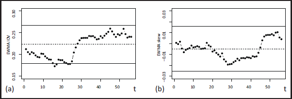
The following data example is inspired by the one in Section 4.2 of Mills (2010), who modelled obesity trends in England for the years in 1993-2005. We consider, however, a much longer period, namely yearly proportions for the period 1975-2016. More precisely, based on the (agestandardized) percentages for different BMI classes (body mass index) offered by the World Health Organization at https://apps.who.int/gho/data/node.main.BMIANTHROPOMETRY?lang=en, the CoTS $x_1,\dots ,x_{42}$ for Germany is derived, with the three categories (hence $d=2$ ) ‘not overweight’ (BMI < 25), ‘overweight’ (BMI in [25;30)), and ‘obese’ (BMI $\ge 30$ ). The data are plotted in Figure 4 (a), where the proportions correspond to the heights of the grey areas (the curves between the grey areas refer to the cumulative proportions). The vertical dashed line between the years 2010 and 2011 expresses the following partition: the data $x_1,\dots ,x_{36}$ for 1975-2010 are used for model fitting, whereas the data $x_{37},\dots ,x_{42}$ for 2011-2016 are left for out-of-sample forecasting.

Looking at Figure 4 (a), an obvious first candidate for modelling the CoTS is a simple (logistic)linear model, that is, (6.1) with

$f_{t,i}=F_{0,1}\left({\eta }_i+{\gamma }_{i}t\right)\text{ for }i=0,\dots ,d-1.$

(6.4)

This is analogous to the model used by Mills (2010) for their UK series, being linear in the components of the alr-transformed data:

$E\left[\text{alr}{\left(x_t\right)}_i\right]=a_i+b_{i}t\text{ for }i=1,\dots ,d.$

(6.5)

Model (6.5) is used as a competitor here. Note that (6.5) could be equivalently expressed in terms of the ilr transform (5.5), which would lead to a reparametrization of the model. Finally, we also consider a version of (6.1) having both a linear trend and a first-order AR-component, namely

$f_{t,i}=F_{0,1}\left({\eta }_i+{\gamma }_{i}t+{\alpha }_1^{\top }{\tilde{X}}_{t-1}\right)\text{ for }i=0,\dots ,d-1.$

(6.6)

The results of CLS estimation (based on $x_1,\dots ,x_{36}$ ) are summarized in Figure 4 (b). The linear coefficients for the fitted ordinal models (6.4) and (6.6) are negative, which is reasonable in view of the decreasing curves for $c_{t,0}=x_{t,0}$ and $c_{t,1}=x_{t,0}+x_{t,1}$ in Figure 4a. The negative linear coefficients for model (6.5) refer to the alr transform (2.1) of the non-cumulative proportions, so they indicate decreasing quotients $x_{t,0}/x_{t,2},x_{t,1}/x_{t,2}$ (if we would use the ilr (5.5) instead of the alr, the parameter estimates of $\left(a_i,b_i\right)$ would change to $\left(0.869,-0.013\right)$ for $i=1$ and $\left(-1.096,0.019\right)$ for $\left.i=2\right)$ . It is also interesting to note that the estimates for $\eta ,\gamma$ are quite similar between models (6.4) and (6.6), that is, one may interpret the estimate of the AR-coefficient ${\alpha }_1$ in (6.6) as a refinement of the baseline linear model (6.4). To compare the performance of the fitted models, two types of CSS are computed: ‘ ${\text{CSS}}_{\text{in }}$ ’ equals ${10}^3$ times the CSS (6.3) computed for the in-sample data $t=2,\dots ,36$ (the summand $t=1$ is left out for all models for a fair comparison, because this summand is not defined for the AR model (6.6)), and ‘ ${\text{CSS}}_{\text{out }}$ ’ equals ${10}^3$ times the CSS (6.3) computed for the out-of-sample data $t=37,\dots ,42$ . Here, the unique scaling factor ${10}^3$ was used to improve the readability of the printed CSS values. It can be seen that the ordinal linear model (6.4) clearly outperforms the linear alrmodel (6.5), because both CSS values of (6.4) are equal to only about $60\text{\%}$ of the (6.5)’s CSS values (the CSS values of the ilr-version of model (6.5) are identical to those of the alr-version). However, a further improvement (especially in terms of the out-of-sample performance) is achieved by the additional AR-term in (6.6). This term, given by ‘ $+0.322X_{t-1,0}-0.651X_{t-1,1}$ ’, shows that the past proportion for ‘not overweight’ has an increasing effect on $f_{t,0},f_{t,1}$ , whereas the one of ‘overweight’ has a decreasing effect. As $\left(x_{t,0}\right)$ strongly decreases for $t=1,\dots ,n$ while $\left(x_{t,1}\right)$ is rather stable, the AR-term becomes increasingly negative over time and, thus, intensifies the linearly decreasing trend in $F_{0,1}^{-1}\left(f_{t,i}\right)$ .

7 Conclusions

This article gave a broad overview of such CoDa areas, where consideration of the natural order of ordinal CoDa might be beneficial. For the (visual) descriptive analysis of ordinal CoDa, for the statistical inference from i. i. d. CoDa samples, for the monitoring of i. i. d. CoDa processes as well as for the modelling of CoDa time series, solutions have been developed and investigated, which make use of the order information in ordinal CoDa. In particular, the asymptotic distribution of diverse ordinal statistics was derived and checked by simulations, the ARL performance of different EWMA control charts was analysed with respect to various out-of-control scenarios, and a novel conditional regression model for ordinal CoTS was successfully applied. Any of the proposed approaches was illustrated with real-world data applications, and the broad variety of such data examples clearly showed the great practical relevance of the new methods.

Because this article was intended to cover a wide a range of subjects, the individual areas were not discussed in too much detail. Thus, for future research, an in-depth analysis of these areas is recommended. Among others, the performance of ordinal CoDa control charts should be investigated also for the case, where serially dependent $\text{CoDa}$ (i. e., time series data) are monitored. Furthermore, it could be tried to adapt methods from ordinal time series analysis (see Weiß, 2020) to the ordinal CoTS case.