A spline-based framework for the flexible modelling of continuously observed multistate survival processes

Abstract

Multistate modelling is becoming increasingly popular due to the availability of richer longitudinal health data. When the times at which the events characterising disease progression are known, the modelling of the multistate process is greatly simplified as it can be broken down in a number of traditional survival models. We propose to flexibly model them through the existing general link-based additive framework implemented in the R package GJRM. The associated transition probabilities can then be obtained through a simulation-based approach implemented in the R package mstate, which is appealing due to its generality. The integration between the two is seamless and efficient since we model a transformation of the survival function, rather than the hazard function, as is commonly found. This is achieved through the use of shape constrained P-splines which elegantly embed the monotonicity required for the survival functions within the construction of the survival functions themselves. The proposed framework allows for the inclusion of virtually any type of covariate effects, including time-dependent ones, while imposing no restriction on the multistate process assumed. We exemplify the usage of this framework through a case study on breast cancer patients.

1 Introduction

When considering multistate processes for the modelling of life-history data, a particularly advantageous setting is that in which transition times are known exactly, that is, the process is continuously observed. In this case, in fact, the overall model likelihood can be decomposed into the product of likelihoods referring to each specific transition only. Estimation then becomes equivalent to fitting one standard survival model for each transition, considering only the subset of the data relevant to that transition and including left-truncation times if the transition at hand can only happen once another has occurred. This is referred to as separate estimation (Putter et al., 2007; Putter, 2011; Crowther and Lambert, 2017). An important practical implication of this is that existing tools can be used to fit the transition-specific models. In particular, we propose to model each transition intensity through the general link-based additive modelling framework by Eletti et al. (2022), implemented in the R package GJRM (Marra and Radice, 2023). This modelling framework allows for the inclusion of virtually any type of covariate effects (including time-dependent effects) using any type of smoother (e.g., thin plate and cubic splines, and tensor products). Importantly, the use of shape constrained P-splines (SCOPs) to model time effects permits to approach the multiple univariate survival models directly on the survival scale, rather than on the hazards scale (which would require expensive numerical integration), while retaining a high degree of modelling flexibility. Specifically, SCOPs, developed by Pya and Wood (2015), extending the penalised B-splines discussed in the seminal work of Eilers and Marx (1996), elegantly embed the monotonicity required for the survival functions within the construction of the survival functions themselves, thus enabling very efficient parameter estimation. The exploration of different forms of dependence on past history also becomes considerably easier when the exact transition times are known. Indeed, assuming a semi-Markov process, the most common relaxation considered in the literature, rather than a Markov process, the most commonly made assumption, implies no further methodological difficulty.

When dealing with life-history data, one is often interested in assessing the effects of specific risk-factors on the probability of transitioning between states. When the process is assumed to be time-dependent and/or not-Markov, the computation of the transition probabilities is a nontrivial task. Two main approaches can be identified in the literature to address this problem and are detailed in Supplementary Material A. We adopt a simulation-based approach which allows one to compute the transition probabilities by simulating a number of paths through the assumed multistate process and counting the number of individuals experiencing each transition (Iacobelli and Carstensen, 2013; Touraine et al., 2016). This is appealing due its aptness at supporting any type of multistate process and was proposed in Fiocco et al. (2008) and implemented, amongst others, in the R package mstate (Putter et al., 2020), whose tools can be seamlessly integrated with the estimation approach implemented in the R package GJRM.

The remainder of the article is organised as follows. In Section 2, the mathematical setting of multistate survival processes is described, while Section 3 introduces the modelling framework. Sections 4, 5 and 6 discuss model estimation, the extraction of the transition probabilities and inference respectively. In Section 7, the Rotterdam Breast Cancer Study is introduced to exemplify the proposed framework. Finally, Section 8 provides some concluding remarks alongside directions of future work.

2 Mathematical setting of multistate survival processes

A continuous-time discrete-state stochastic process is a family of random variables $\{Z(t),t\in \mathcal{T}\}$ with some indexing set given by $\mathcal{T}=[\mathrm{0,}\infty )$ in the survival setting. The set of all values that the process takes $\mathcal{S}:=\{z:Z(t)=z\mathrm{,}t\in \mathcal{T}\}\subseteq \left\{\mathrm{0,1,2,...}\right\}$ is called the state space, where $Z(t)$ denotes the state occupied at time t. A $p\times 1$ vector of left-continuous, time-dependent covariates is represented by $X(t)$ . The history of the process, including the evolution of the covariates vector, is denoted by ${\mathcal{F}}_t=\{Z(u),X(u),0\le u\le t\}$ . The transition intensities and the transition probabilities are then the two key quantities associated with the process. The former represent the rates of transition to a state $s$ for an individual who is currently in another state $r$ , formally

$$q^{(rs)}(t|{\mathcal{F}}_{t^{-}})=\underset{\Delta t\downarrow 0}{{\displaystyle \lim }}\frac{P(Z(t+\Delta t^{-})=s|Z(t^{-})=r\mathrm{,}{\mathcal{F}}_{t^{-}})}{\Delta t}\mathrm{,}r\ne s\mathrm{,}$$

with $q^{(rs)}(t|{\mathcal{F}}_{t^{-}})=0$ if r is an absorbing state and $q^{(rr)}(t|{\mathcal{F}}_{t^{-}})=-{\displaystyle \sum _{s\ne r}}{q}^{(rs)}(t|{\mathcal{F}}_{t^{-}})$ . The matrix with $(r\mathrm{,}s)$ element given by $q^{(rs)}(t|{\mathcal{F}}_{t^{-}})$ for every $r\mathrm{,}s\in \mathcal{S}$ is called transition intensity matrix or generator matrix and we will denote it by $Q(t|{\mathcal{F}}_{t^{-}})$ . Similarly, we define the transition probability matrix associated with the time interval $[u\mathrm{,}t]$ as the matrix with $(r\mathrm{,}s)$ element given by $P(Z(t)=s|Z(u)=r\mathrm{,}{\mathcal{F}}_{u^{-}})$ and denote this by $P(u\mathrm{,}t|{\mathcal{F}}_{u^{-}})$ . It is common to simplify the dependence on past history and time by assuming either a Markov or a semi-Markov process. The former implies that the probability of being in a given state at a given future time only depends on the current state occupied (Ross et al., 1996). The latter assumes that the future state only depends on the history of the process through the current state and through time since entry to the current state (Pyke, 1961; Yang and Nair, 2011). Exact knowledge of the transition times, as in our setting, allows for both assumptions to be modelled in an equally straightforward manner. The time for intermediate transitions will just need to be re-defined to be the time from entry to the current state.

3 Flexible transition-specific modelling

When a multistate process is continuously observed, each transition time can be viewed as a standalone time-to-event and can thus be modelled through traditional survival analysis. It is well know that survival analysis can be undertaken on different scales. One such option is to model transformations of the survival function using generalised survival models, a class that was first introduced by Younes and Lachin (1997). Subsequent works further developed this approach (e.g., Royston and Parmar, 2002; Liu et al., 2018), each allowing for more modelling flexibility and ensuring the monotonicity of the survival function in different ways. More recently Marra and Radice (2020) proposed a generalised survival modelling framework which elegantly embeds the monotonicity of the survival function within the model design matrix by exploiting the properties of P-splines (see Section 3.2). We adopt this approach and thus describe it in the following in the context of transition-specific modelling.

Let $\mathcal{A}=\{(r\mathrm{,}s)|r\ne s\in \mathcal{S}\mathrm{,}{q}^{(rs)}(t_i)\ne 0\}$ be the set of transitions and $N$ represent the sample size. For observation $i=\mathrm{1,}\dots \mathrm{,}n$ and for $(r\mathrm{,}s)\in \mathcal{A}$ , let $H^{(rs)}(\cdot )$ be the cumulative transition-specific hazard defined in terms of the transition intensity $q^{(rs)}(\cdot )$ as $H^{(rs)}(t_i|x_i;{\beta }^{(rs)})={\displaystyle \underset{0}{\overset{t_i}{\int }}}{q}^{(rs)}(u|x_i;{\beta }^{(rs)})du$ . Then we will have a conditional survival function denoted by $S^{(rs)}(t_i|x_i;{\beta }^{(rs)})=\exp \left\{-H^{(rs)}(t_i|x_i;{\beta }^{(rs)})\right\}\in (\mathrm{0,1})$ , where $x_i$ represents a generic vector of patient characteristics that has an associated regression coefficient vector ${\beta }^{(rs)}\in {ℝ}^w$ , where $w$ is the length of ${\beta }^{(rs)}$ . A link-based additive transition-specific survival model can then be written as

$$g\left\{S^{(rs)}(t_i|x_i;{\beta }^{(rs)})\right\}={\eta }_i^{(rs)}(t_i\mathrm{,}{x}_i;f({\beta }^{(rs)})),$$

(3.1)

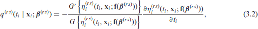
where $g:(\mathrm{0,1})\to ℝ$ is a monotone and twice continuously differentiable link function with bounded derivatives, hence invertible, which determines the scale of the analysis, ${\eta }_i^{(rs)}(t_i\mathrm{,}{x}_i;f({\beta }^{(rs)}))\in ℝ$ is an additive predictor which includes a baseline function of time and several types of covariate effects and $f({\beta }^{(rs)})$ is a vector function of ${\beta }^{(rs)}$ through which the monotonicity required for the survival functions is imposed (see Section 3.2). Rearranging (1) yields $S^{(rs)}(t_i|x_i;{\beta }^{(rs)})=G\left\{{\eta }_i^{(rs)}(t_i\mathrm{,}{x}_i;f({\beta }^{(rs)}))\right\}$ , where $G$ is an inverse link function. Note that modelling directly on the survival scale implies a considerable advantage in this context (see Section 5). The cumulative transition-specific hazard is then $H^{(rs)}(t_i|x_i;{\beta }^{(rs)})=-\log \left[G\left\{{\eta }_i^{(rs)}(t_i\mathrm{,}{x}_i;f({\beta }^{(rs)}))\right\}\right]$ and the transition intensity function is defined as

$$q^{(rs)}(t_i|x_i;{\beta }^{(rs)})=-\frac{G^{\prime }\left\{{\eta }_i^{(rs)}(t_i\mathrm{,}{x}_i;f({\beta }^{(rs)}))\right\}}{G\left\{{\eta }_i^{(rs)}(t_i\mathrm{,}{x}_i;f({\beta }^{(rs)}))\right\}}\frac{\partial {\eta }_i^{(rs)}(t_i\mathrm{,}{x}_i;f({\beta }^{(rs)}))}{\partial t_i}\mathrm{,}$$

(3.2)

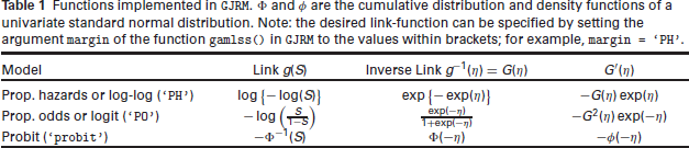
where $G^{\prime }\left\{{\eta }_i^{(rs)}(t_i\mathrm{,}{x}_i;f({\beta }^{(rs)}))\right\}=\partial G\left\{{\eta }_i^{(rs)}(t_i\mathrm{,}{x}_i;f({\beta }^{(rs)}))\right\}/\partial {\eta }_i^{(rs)}(t_i\mathrm{,}{x}_i;f({\beta }^{(rs)}))$ . Table 1 displays the functions $g$ , $G$ and $G^{\prime }$ available in the R package GJRM.

Table 1

Functions implemented in GJRM. $\Phi$ and $\varphi$ are the cumulative distribution and density functions of a univariate standard normal distribution. Note: the desired link-function can be specified by setting the argument margin of the function gamlss() in GJRM to the values within brackets; for example, margin = ‘PH’.

Model	Link $g(S)$	Inverse Link $g^{-1}(\eta )=G(\eta )$	$G^{\prime }(\eta )$
Prop. hazards or log-log (‘PH’)	$\log \left\{-\log (S)\right\}$	$\exp \left\{-\exp (\eta )\right\}$	$-G(\eta )\exp (\eta )$
Prop. odds or logit (‘PO’)	$-\log \left(\frac{S}{1-S}\right)$	$\frac{\exp (-\eta )}{1+\exp (-\eta )}$	$-G^2(\eta )\exp (-\eta )$
Probit (‘probit’)	$-{\Phi }^{-1}(S)$	$\Phi (-\eta )$	$-\varphi (-\eta )$

3.1 Additive predictor

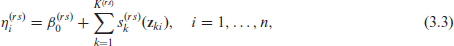
Dropping the dependence on covariates and on parameters for the sake of simplicity, the additive predictor is defined as

$${\eta }_i^{(rs)}={\beta }_0^{(rs)}+{\displaystyle \sum _{k=1}^{K^{(rs)}}}{s}_k^{(rs)}(z_{ki}),i=\mathrm{1,}\dots \mathrm{,}n\mathrm{,}$$

(3.3)

where ${\beta }_0^{(rs)}\in ℝ$ is an overall intercept, $z_{ki}$ denotes the $k^{th}$ sub-vector of the complete vector $z_i$ and the $K^{(rs)}$ functions $s_k^{(rs)}(z_{ki})$ denote effects which are chosen according to the type of covariate(s) considered. These functions can be expressed as a linear combination of basis functions $b_k(z_{ki})=(b_{k1}^{(rs)}(z_{ki}),\dots \mathrm{,}{b}_{k{J}_k}^{(rs)}(z_{ki}{))}^T$ and regression coefficients $f_k^{(rs)}({\beta }_k^{(rs)})=(f_{k1}^{(rs)}({\beta }_{k1}^{(rs)}),\dots$ , $f_{k{J}_k}^{(rs)}({\beta }_{k{J}_k}^{(rs)}{))}^T\in {ℝ}^{J_k}$ , that is $s_k^{(rs)}(z_{ki})=b_k{(z_{ki})}^T{f}_k^{(rs)}({\beta }_k^{(rs)})$ (e.g., Wood, 2017). We can then write (3) compactly as ${\eta }_i^{(rs)}=Z_i^{(rs)T}{f}^{(rs)}({\beta }^{(rs)})$ , where $Z_i^{(rs)}=(\mathrm{1,}{b}_1{(z_{1i})}^T\mathrm{,}\dots \mathrm{,}{b}_{K^{(rs)}}{(z_{K^{(rs)}i})}^T{)}^T$ and $f^{(rs)}({\beta }^{(rs)})=({\beta }_0^{(rs)}\mathrm{,}{f}_1^{(rs)}{({\beta }_1^{(rs)})}^T\mathrm{,}\dots \mathrm{,}{f}_{K^{(rs)}}^{(rs)}{({\beta }_{K^{(rs)}}^{(rs)})}^T{)}^T$ . Observe that $\partial {\eta }_i^{(rs)}(t_i\mathrm{,}{x}_i;f^{(rs)}({\beta }^{(rs)}))/\partial t_i$ is required in (2). This can be expressed as $Z_i^{(rs)}{(t_i\mathrm{,}{x}_i)}^{\text{'}T}{f}^{(rs)}({\beta }^{(rs)})$ where, depending on the type of spline basis employed, $Z_i(t_i\mathrm{,}{x}_i{)}^{\prime }=\underset{\epsilon \to 0}{\lim }\frac{Z_i^{(rs)}(t_i+\epsilon \mathrm{,}{x}_i)-Z_i^{(rs)}(t_i-\epsilon \mathrm{,}{x}_i)}{2\epsilon }$ can be calculated either by a finite-difference method or analytically. Each ${\beta }_k^{(rs)}$ has an associated quadratic penalty ${\text{λ}}_k^{(rs)}{\beta }_k^{(rs)T}{D}_k^{(rs)}{\beta }_k^{(rs)}$ , used in fitting, whose role is to enforce specific properties on the $k^{th}$ function, such as smoothness, with matrix $D_k^{(rs)}$ depending only on the choice of the basis functions. The smoothing parameter ${\text{λ}}_k^{(rs)}\in [\mathrm{0,}\infty )$ controls the trade-off between fit and smoothness, and hence determines the shape of the estimated smooth function. The overall penalty can be defined as ${\beta }^{(rs)T}{S}_{{\text{λ}}^{(rs)}}^{(rs)}{\beta }^{(rs)}$ , where $S_{{\text{λ}}^{(rs)}}^{(rs)}=\text{diag}(0,{\text{λ}}_1^{(rs)}{D}_1^{(rs)},\dots ,{\text{λ}}_{K^{(rs)}}^{(rs)}{D}_{K^{(rs)}}^{(rs)})$ is a block diagonal matrix where each block is given by the $k^{th}$ penalty, and where ${\text{λ}}^{(rs)}=({\text{λ}}_1^{(rs)}\mathrm{,}\dots \mathrm{,}{\text{λ}}_{K^{(rs)}}^{(rs)}{)}^T$ is the transition-specific overall smoothing parameter vector. Depending on the types of covariate effects one wishes to model, several definitions of basis functions are possible, for example, thin plate, cubic and P- regression splines, tensor products, Markov random fields, random effects, Gaussian process smooths. These are handled automatically within the software proposed. We refer the reader to Section 7 for practical examples of the effects mentioned above and to Wood (2017) for the other available options.

3.2 Imposing monotonicity by means of SCOPs

When modelling life-history data through multistate processes, one is often interested in making statements in terms of the probabilities of transitioning from one state to another for specific combinations of risk-factors. In Section 5, it will be shown that we compute these by first extracting the transition-specific cumulative hazards at various time points. Direct modelling of the survival functions thus allows us to obtain the transition probabilities more cheaply, as we drop the intermediate step of having to first integrate the transition intensities. The only caveat is that one needs to ensure the survival functions are monotonically decreasing. Liu et al. (2018) propose to do this by means of a penalty applied to the hazard function such that the associated coefficient is iteratively doubled until the estimated hazard functions of all individuals are not negative. We employ a more theoretically founded approach. Indeed, in the proposed framework the properties of P-splines are exploited to elegantly embed the monotonicity within the construction of the survival functions themselves, while allowing for the flexible modelling of the time effect.

Let $s^{(rs)}(t_i)={\displaystyle {\sum }_{j=1}^{J^{(rs)}}}{f}_j^{(rs)}({\beta }_j^{(rs)})b_j^{(rs)}(t_i)$ , where the $b_j^{(rs)}(\cdot )$ are B-spline basis functions of at least second order built over the interval $[a\mathrm{,}b]$ , based on equally spaced knots, and the $f_j^{(rs)}{({\beta }_j)}^{(rs)}$ are spline coefficients. Given the link functions listed in Table 1, we need $s^{(rs{)}^{\prime }}(t_i)\ge 0$ . Eilers and Marx (1996) combined B-spline basis functions with discrete penalties in the basis coefficients to produce the popular P-spline smoothers. Then Pya and Wood (2015) proposed shape constrained P-splines through a mildly nonlinear extension of these P-splines, with corresponding novel discrete penalties, thus allowing the development of efficient and stable model estimation frameworks, such as the one proposed. In particular, a sufficient condition for $s^{(rs{)}^{\prime }}(t_i)\ge 0$ over $[a\mathrm{,}b]$ is that $f_j^{(rs)}({\beta }_j^{(rs)})\ge f_{j-1}^{(rs)}({\beta }_{j-1}^{(rs)}),\forall j$ . Indeed, given a function $\eta (x)=a_0+{\displaystyle {\sum }_{j=1}^m}{a}_j{B}_j(x\mathrm{,}q)$ , where $B_j(x\mathrm{,}q)$ are the bases for a ${(q+1)}^{th}$ order B-spline, m is the number of basis functions, $\partial \eta (x)/\partial x=\frac{1}{h}{\displaystyle {\sum }_{j=1}^{m-1}}(a_{j+1}-a_j)B_j(x\mathrm{,}q-1)$ with $h$ the distance between equally spaced knots and so $a_{j+1}\ge a_j$ implies $\partial \eta (x)/\partial x\le 0$ since $B_j(x\mathrm{,}q-1)\ge 0$ (Leitenstorfer and Tutz, 2007). Such condition can be imposed by defining the vector function $f^{(rs)}({\beta }^{(rs)})=\Sigma {\left\{{\beta }_1^{(rs)}\mathrm{,}\exp ({\beta }_2^{(rs)}),\dots \mathrm{,}\exp ({\beta }_{J^{(rs)}}^{(rs)})\right\}}^T$ , where $\Sigma [{\iota }_1\mathrm{,}{\iota }_2]=0$ if ${\iota }_1<{\iota }_2$ and $\Sigma [{\iota }_1\mathrm{,}{\iota }_2]=1$ if ${\iota }_1\ge {\iota }_2$ , with ${\iota }_1$ and ${\iota }_2$ denoting the row and column entries of $\Sigma$ , and ${\beta }^{(rs)T}=({\beta }_1^{(rs)}\mathrm{,}{\beta }_2^{(rs)}\mathrm{,}\dots \mathrm{,}{\beta }_{J^{(rs)}}^{(rs)})$ is the parameter vector to estimate. Crucially, in practice $\Sigma$ is absorbed into the design matrix containing the B-spline basis functions Z, hence allowing the constraint to be elegantly embedded within the construction of the model design matrix itself. Finally, in a smoothing context, we are interested in having a penalty on the smooth function to control its ‘wiggliness’. Eilers and Marx (1996) introduced the notion of directly penalising the difference in the basis coefficients of a B-splines basis, which is used with a relatively large number of basis functions to avoid underfitting. The adaptation to the shape-constrained case is straightforward as it implies penalising the squared differences between adjacent ${\beta }_j^{(rs)}$ , starting from ${\beta }_2^{(rs)}$ , using $D^{(rs)}=D^{(rs)*T}{D}^{*}$ where $D^{(rs)*}$ is a $(J^{(rs)}-2)\times J^{(rs)}$ matrix made up of zeros except that $D^{(rs)*}[\iota \mathrm{,}\iota +1]=-D^{(rs)*}[\iota \mathrm{,}\iota +2]=1$ for $\iota =\mathrm{1,}\dots \mathrm{,}{J}^{(rs)}-2$ . The penalty is zeroes when all the ${\beta }_j^{(rs)}$ after ${\beta }_1^{(rs)}$ are equal so that the $f_j^{(rs)}({\beta }_j^{(rs)})$ form a uniformly increasing sequence and $s^{(rs)}(t_i)$ is an increasing straight line. As a result, the proposed penalty shares the basic feature of smoothing towards a straight line, but in a manner that is computationally convenient for constrained smoothing.

4 Estimation

Since each likelihood contribution refers to a specific transition only and every transition is exactly observed if and only if it occurs, it can be shown (see Supplementary Material B) that the overall model log-likelihood can be broken down into the sum of the log-likelihoods associated with each transition, which are functions only of the parameters relating to that transition, that is, $\mathcal{l}(\theta )={\displaystyle {\sum }_{(r\mathrm{,}s)\in \mathcal{A}}}{\mathcal{l}}^{(rs)}({\beta }^{(rs)})$ , where $\theta =\left\{{\beta }^{(rs)}\right|(r\mathrm{,}s)\in \mathcal{A}\}$ is an overall model parameter vector. Re-writing the log-likelihood in this way, rather than as a sum of contributions associated with each observation time, is more convenient as it breaks down the estimation task into a number of traditional survival problems, one for each transition. It is precisely to each of these transition-specific models that the framework developed in Eletti et al. (2022) is applied. Briefly, as the model allows for a high degree of flexibility, to prevent over-fitting, the log-likelihood is augmented with a penalty term ${\mathcal{l}}_p^{(rs)}({\beta }^{(rs)})={\mathcal{l}}^{(rs)}({\beta }^{(rs)})-\frac{1}{2}{\beta }^{(rs)T}{S}_{{\lambda }^{(rs)}}^{(rs)}{\beta }^{(rs)}$ where $S_{{\text{λ}}^{(rs)}}^{(rs)}$ is an overall penalty term defined in Section 3. The estimation framework then combines a carefully structured trust region algorithm which uses the analytical expressions of the gradient and Hessian of the log-likelihood and properly chosen starting values with a general automatic multiple smoothing parameter selection algorithm based on an approximate AIC measure.

5 Prediction on the transition probabilities scale

While estimation can be carried out entirely by-passing the computation of the transition probabilities, one is often interested in making statements in terms of the probability of transitioning from one state to another given a specific combination of risk-factors. We choose the simulation-based approach proposed in Fiocco et al. (2008), which we briefly describe in the following. Let r be the starting state, entered at time $t_r=0$ , and $t_{\text{max}}$ the maximum follow-up time. Then

• Let $\mathcal{B}$ be the set of states that can be reached from state r. If $\mathcal{B}$ is empty, stop. Otherwise, for $s\in \mathcal{B}$ , let $H^{(rs)}(t)$ be the cumulative transition-specific hazard function for transition $r\to s$ and $H^{(r\cdot )}(t)={\displaystyle \sum _{s\in \mathcal{B}}}{H}^{(rs)}(t)$ refer to the event of leaving state $r$ .

• Sample $t^{*}$ from $H^{(r\cdot )}(t)-H^{(r\cdot )}(t_r)$ . This refers to the conditional distribution of leaving state $r$ given that the process is known to be in state $r$ until time $t_r$ thus ensuring that the sampled time $t^{*}>t_r$ .

• If $t^{*}>t_{max}$ , select the next state $s$ with probability $d{H}^{(rs)}(t^{*})/d{H}^{(r\cdot )}(t^{*})$ , which provides a weight for the specific transition $r\to s$ out of state $r$ for each $s\in \mathcal{B}$ at the given time $t^{*}$ , and set the new starting points for the next iteration, $r=s$ and $t_r=t^{*}$ . Otherwise, stop: a full path through the process was obtained.

This is repeated to obtain M paths through the multistate model and to compute the transition probabilities by counting the number of paths for which each event occurred. This approach is implemented in the function mssample() of the R package mstate and is straightforward to use given the estimated transition-specific cumulative hazards for both Markov and semi-Markov models.

6 Inference

One view of the smoothing process is that the penalty employed during fitting imposes the belief that the true function is more likely to be smooth than wiggly. This belief can be expressed in a Bayesian manner through the form of a prior distribution on ${\beta }^{(rs)}$ , that is, $f_{{\beta }^{(\text{rs})}}\propto \exp \left\{-{\beta }^{(rs)T}{S}_{{\lambda }^{(rs)}}^{(rs)}{\beta }^{(rs)}/2\right\}$ . This leads to the Bayesian large sample approximation ${\beta }^{(rs)}\stackrel{\cdot }{\sim }\mathcal{N}({\widehat{\beta }}^{(rs)}\mathrm{,}{V}_{{\beta }^{(rs)}})$ , where $V_{{\beta }^{(rs)}}=-H_p{({\widehat{\beta }}^{(rs)})}^{-1}$ ; using $V_{{\beta }^{(rs)}}$ gives close to across-the-function frequentist coverage probabilities because it accounts for both sampling variability and smoothing bias, a feature that is particularly relevant at finite sample sizes (Wood et al., (2016). Following Pya and Wood (2015), we then consider the Taylor series expansion of $f^{(rs)}({\beta }^{(rs)})$ around $f^{(rs)}({\tilde{\beta }}^{(rs)})$ . This gives $f^{(rs)}({\beta }^{(rs)})-f^{(rs)}({\tilde{\beta }}^{(rs)})\approx \text{diag}(E^{(rs)})({\beta }^{(rs)}-{\tilde{\beta }}^{(rs)})$ , where $E^{(rs)}[k_{j_k}]=1$ if $f_{k_{j_k}}^{(rs)}({\beta }_{k_{j_k}}^{(rs)})={\beta }_{k_{j_k}}$ and $\exp ({\beta }_{k_{j_k}}^{(rs)})$ otherwise, showing that $f^{(rs)}({\beta }^{(rs)})-f^{(rs)}({\tilde{\beta }}^{(rs)})$ is approximately a linear function of ${\beta }^{(rs)}$ . Combining this with the result above we have that $f^{(rs)}({\beta }^{(rs)})\stackrel{\cdot }{\sim }\mathcal{N}(f^{(rs)}({\tilde{\beta }}^{(rs)}),V_{f^{(rs)}({\beta }^{(rs)})})$ where $V_{f^{(rs)}({\beta }^{(rs)})}=\text{diag}(E^{(rs)})V_{{\beta }^{(rs)}}\text{diag}(E^{(rs)})$ , since linear functions of normally distributed random variables follow normal distributions. Confidence intervals for linear functions of the model coefficient can then be obtained using this result. P-values for the smooth components in the model are derived by adapting the result discussed in Wood (2017) and using $V_{f^{(rs)}({\beta }^{(rs)})}$ as covariance matrix. For nonlinear functions of the model coefficients, for example, the transition-specific cumulative hazard functions, instead, the intervals can be conveniently obtained by posterior simulations, hence avoiding computationally expensive parametric bootstrap or frequentist approximations, for instance.

7 Primary breast cancer modelling case study

To illustrate what the proposed approach adds compared to the existing literature, we consider the case study described in Crowther and Lambert (2017) which is based on data from 2892 patients with primary breast cancer for which the time to relapse and/or the time to death is known. See, for example, Sauerbrei et al. (2007) for further details on the Rotterdam Breast Cancer Study from which the data originated. The code used to produce this analysis can be found in the public repository https://github.com/AlessiaEletti/ContinObsMultistateProcesses . All patients begin in the initial post-surgery state, 1518 patients experience relapse, 195 die without relapse and 1075 die after experiencing relapse. A Markov illness-death model (IDM, see Figure 5 in Supplementary Material C) will thus be used to model the data. As an aside, note that an attempt assuming semi-Markovianity was also made but this was not supported by the data according to the AIC values found for the fitted models. As there are three transitions in the assumed IDM, three survival models will be fitted. For transitions which can occur only given that another transition has already taken place, that is, the transition $2\to 3$ in this case, one must account for the fact that the patient is at risk only after entering the new starting state, that is, state 2. As long as this is done, each transition can be treated as a separate survival problem. The time at which the individual entered state 2 thus becomes the left-truncation time for the new transition $2\to 3$ . To clarify how the separate estimations are carried out, recall that longitudinal survival data are characterised by multiple observations through time of at least one quantity of interest for the same individual. Typically the data are formatted in the so-called stacked (or long) form, that is, each row represents a single time point per subject. In particular, each subject will have at least $v$ rows, where $v$ is the number of possible transitions exiting the initial state. Here, $v=2$ as there are two ways of exiting state 1, that is, going in state 2 or 3. A start and a stop time will then indicate, respectively, the first time after which the patient becomes at risk of the given transition and the time at which the transition itself occurred. The start time for transitions exiting the first state is 0, as is usually the case here. If the patient transitions to an intermediate state, $u$ rows will be added, where $u$ is the number of transitions exiting the intermediate transition state reached. Here, $u=1$ , as the only possible transition out of state 2 is $2\to 3$ , where 3 is an absorbing state. When estimating $q^{(12)}(\cdot )$ , all of the rows relating to this transition are included in the estimation. Since every patient will at least have one row for each transition exiting the first state, this implies that the entire population is included. The same is true for $q^{(13)}(\cdot )$ , for which the rows relating to the $1\to 3$ transition will be used for estimation. The two resulting separate datasets can then be treated as traditional survival data with uncensored and right-censored observations and with the event of interest given by the transition to the new state, that is, state 2 for the former and state 3 for the latter. When estimating $q^{(23)}(\cdot )$ , only individuals who have transitioned to state 2 at some point are included in the estimation. The data are then treated as traditional survival data with left-truncated uncensored and left-truncated right-censored observations and where the event of interest is the transition to the absorbing state 3. We refer the reader to Supplementary Material D for further details on the format of the data in this setting.

The dataset contains information on the age of the patient at primary surgery (in years), tumour size (divided into 3 classes: $\le 20$ , $20-50$ and $>50$ mm), number of positive nodes, progesterone levels (in fmol/L) and whether or not the patient was on hormonal therapy. These are all included as covariates. We then include a time-dependent effect for the progesterone level, as this has been found to be relevant in the reference paper, and include age, the progesterone level and the number of positive nodes nonlinearly, as supported by existing literature. Importantly, our chosen framework allows for the exploration of these effects in a more general and flexible manner than previously possible in the literature thanks to the use of splines. In contrast, for instance, Sauerbrei and Royston (1999) modelled the number of positive nodes nonlinearly by using fractional polynomials with the degrees set heuristically. Similarly, in Crowther and Lambert (2017) the time-dependant effect is captured by a single interaction coefficient between time and the progesterone level. In particular, for $(r\mathrm{,}s)\in \{(\mathrm{1,2}),(\mathrm{1,3}),(\mathrm{2,3})\}$ , we specify the transition-specific models

$$\begin{array}{c}{\eta }_i^{(rs)}(t_i\mathrm{,}{x}_i;f({\beta }^{(rs)}))={\beta }_0^{(rs)}+s_0^{(rs)}(\log ({\text{t}}_i))+{\beta }_1^{(rs)}{\text{I}}_{{\text{size}}_i=20-50}+{\beta }_2^{(rs)}{\text{I}}_{{\text{size}}_i>50}+{\beta }_3^{(rs)}{\text{hormon}}_i\\ +s_1^{(rs)}({\text{age}}_i)+s_2^{(rs)}({\text{nodes}}_i)+s_3^{(rs)}({\text{pr}}_i)+s_4^{(rs)}(\log ({\text{t}}_i),{\text{pr}}_i),\end{array}$$

where $s_0^{(rs)}(\log ({\text{t}}_i))$ is a monotonic P-spline of the logarithm of time which ensures the monotonicity of the survival function associated with this transition, as explained in Section 3.2; $s_1^{(rs)}({\text{age}}_i)$ , $s_2^{(rs)}({\text{nodes}}_i)$ and $s_3^{(rs)}({\text{pr}}_i)$ are thin-plate splines, while $s_4^{(rs)}(\log ({\text{t}}_i),{\text{pr}}_i)$ is a pure smooth interaction between time and the progesterone level, that is, a time-dependent effect. In regard to the penalty associated with a nonlinear term, for example, $s_1({\text{age}}_i)$ , this takes the form of the quadratic penalty defined above with $D_k$ given by the integrated square second derivative of the basis functions, that is, ${\displaystyle \int }{d}_k(z_k)d_k{(z_k)}^{T}d{z}_k$ with the $j_k^{th}$ element of $d_k(z_k)$ defined as ${\partial }^2{b}_{k{j}_k}(z_k)/\partial z_k^2$ . The penalty associated with the time-dependent effect is, instead, more complex as it entails combining two penalties (see Wood, 2017, Chapter 5). Finally, note that for parametric effects the spline representation simplifies to $s^{(rs)}({\text{hormon}}_i)={\beta }_3^{(rs)}{\text{hormon}}_i$ . No penalty is typically assigned to parametric effects, hence the associated quadratic penalty is $D=0$ . Note that in cases such as those in which the categorical variable has many levels with some with few observations, it may be advisable to set the penalty as the identity matrix. In this way, a ridge penalty is imposed and it may help avoid that the parameters associated with the more sparse categories are weakly or nonidentified.

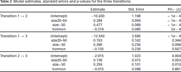
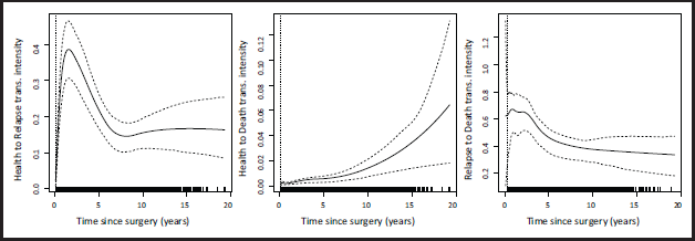
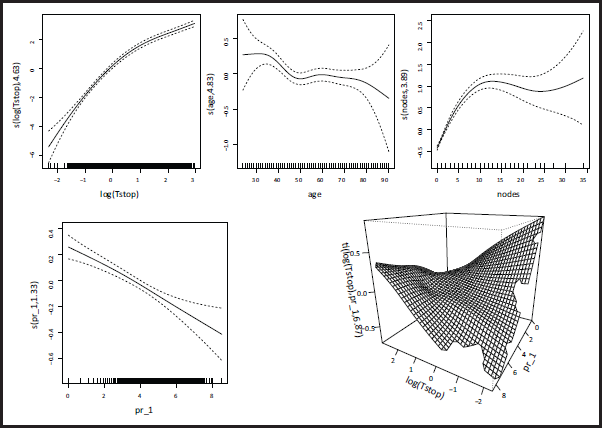
The estimated covariate effects for each transition are reported in Table 2. For the first transition, for instance, they are all significant and in line with our expectations: the larger the size of the tumor the higher the risk of experiencing relapse, while hormonal therapy has a beneficial effect. In Figure 1 we report the estimated transition intensities with their 95% confidence intervals as functions of time for a 54 year old patient with tumour size $\ge 50$ mm, 10 positive nodes, progesterone level of 3 and under hormonal therapy. We find, for instance, that the risk of experiencing relapse for this profile increases for approximately 2.5 years after surgery, then it decreases and plateaus over time. In Figure 2 we report the plots of the smooths and of the tensor interaction for the transition $health\to relapse$ . These show that the data particularly support nonlinear effects for the age and the number of positive nodes. For instance, the latter exhibits an increasing trend up to about 12 nodes, followed by a plateau. The time-dependence of the progesterone level effect is also clear from the surface representing the smooth interaction, with low levels of progesterone associated with a decreasing risk of experiencing relapse over time and, conversely, high levels of progesterone associated with an increasing trend for the risk of experiencing relapse over time. Any additional complexity not supported by the data is then suppressed automatically through the estimation of the smoothing parameter, rather than requiring the user to make restrictive and potentially arbitrary choices a priori. This can be seen in the plots of the smooths of the remaining two transitions, reported in Figures 6 and 7 of Supplementary Material C. The plot of the smooth of age for the $health\to death$ transition, for instance, shows that the data actually supported a linear effect for this term.

Table 2

Model estimates, standard errors and p-values for the three transitions.

		Estimate	Std. Error	Pr( $>\left|z\right|$ )
Transition $1\to 2$	(Intercept)	$-$ 10.630	1.198	$<1e-4$
	size20–50	0.284	0.059	$<1e-4$
	size $>$ 50	0.477	0.089	$<1e-4$
	hormon	$-$ 0.318	0.085	$2e-4$
Transition $1\to 3$	(Intercept)	$-$ 12.543	2.585	$<1e-4$
	size20–50	0.153	0.162	0.344
	size $>$ 50	0.390	0.236	0.098
	hormon	$-$ 0.135	0.236	0.567
Transition $2\to 3$	(Intercept)	$-$ 2.915	1.023	0.004
	size20–50	0.139	0.072	0.053
	size $>$ 50	0.259	0.101	0.010
	hormon	$-$ 0.015	0.098	0.881

Figure 1

Fitted transition intensities and 95% confidence intervals (CIs) for a 54 year old patient under hormonal therapy with tumour size $\ge 50$ mm, 10 nodes and progesterone level of 3, over 20 years. The vertical dashed line marks the smallest observed time: the transition intensities estimated at smaller times are extrapolations, thus explaining the wide CIs in the first section of the third plot. The width of the CIs in the final portion of the middle plot can be explained by the scarcity of observations in the final times, as shown by the rug plot. The width of the confidence intervals should also be related to the different range of values in each plot.

Figure 2

Smooth of log-time (top left), smooth of age (top middle), smooth of the number of positive nodes (top right), smooth of the progesterone level (bottom left) and smooth interaction between log-time and progesterone level (bottom right) for the transition $health\to relapse$ .

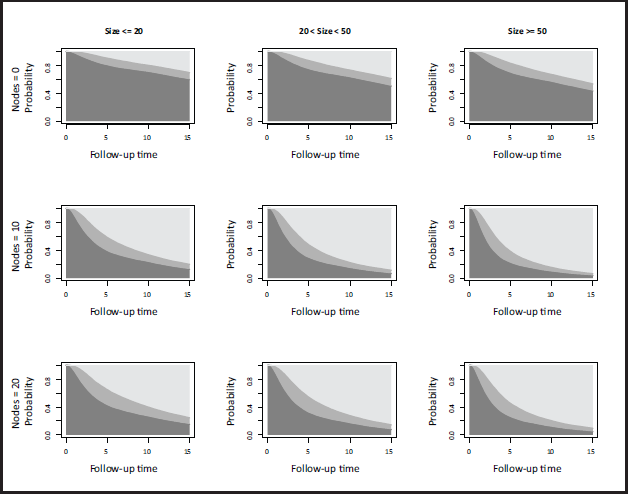
As mentioned above, interest usually lies in making statements in terms of the probabilities of transitioning between states thus, in Figure 3, we report stacked transition probability plots. Representing the probabilities in this stacked manner is a common way of quickly providing an overview of how risk evolves over time, however the uncertainty of the estimates cannot be easily portrayed. For this reason, in Figure 4, we report the predicted probabilities with their 95% confidence intervals for the individual corresponding to the top-left panel, that is, a 54 year old patient under hormonal therapy, progesterone level of 3, 20 positive nodes and tumour size $\le 20$ mm. Note that the computation of the transition probabilities already entails a simulation, thus the process of obtaining confidence intervals for it will result in two nested simulations. The computational burden of this is not prohibitively high, however. Here, they are obtained by using 100 simulated cumulative hazards for each of the three transitions, over 100 distinct time points, and $M=10000$ simulated paths through the process, which is a larger number of paths than typically needed. This required approximately 37 minutes using a laptop with Windows 10 (2.20 GHz processor, 16 GB RAM, 64-bit). Details on this, on how the model fitting is carried out and how the plots reported in this section were obtained can be found in Supplementary Material C.

Figure 3

Stacked representation of estimated transition probabilities (dark grey: post-surgery; grey: relapse; light grey: death) for each combination of nodes (0, 10 and 20) and tumour sizes ( $\le 20$ , $(\mathrm{20,50})$ and $\ge 50$ ) considered in a 54 year old patient under hormonal therapy with progesterone level of 3.

Figure 4

Estimated transition probabilities (left: post-surgery; middle: relapse; right: death) for the top-left pane in Figure 3.

8 Discussion

In this work we show how one can use existing tools to flexibly model multistate survival processes relating to continuously observed life-history data. In particular, we consider the survival estimation framework described in Eletti et al. (2022) and implemented in the R package GJRM which allows us to model virtually any type of covariate effect, including time-dependent ones. Direct modelling of the survival functions implies a considerable gain in efficiency when it comes to computing the transition probabilities of interest, which in turn are obtained through a simulation-based approach able to support any type of multistate process. Efficient modelling on the survival scale is achieved through shape constrained P-splines, developed by Pya and Wood (2015), building upon the work done in Eilers and Marx (1996). We exemplify our approach on data from the Rotterdam Breast Cancer Study and provide the code used for the analysis in the public repository https://github.com/AlessiaEletti/ContinObsMultistateProcesses .

With regard to directions of future work, we are interested in integrating the computation of the transition probabilities and the extraction of its confidence intervals directly within the GJRM package, so as to minimise the amount of user-written code needed and thus further simplify the use of these models by the practitioner. Similarly, for the visualisation tools available for the estimated transition probabilities. As the Markov assumption is quite common, we are also interested in implementing the method based on the numerical solution of the differential equations tying the transition probabilities to the intensities as well as to implement our own simulation-based approach within the GJRM package, so that the user has all necessary instruments in the same place and the need for user-written code is reduced to the minimum.

Supplementary materials

Supplementary materials for this article are available online.

Supplemental Material for A spline-based framework for the flexible modelling of continuously observed multistate survival processes by Alessia Eletti, Giampiero Marra and Rosalba Radice, in Statistical Modelling