
Abstract
For health-economic analyses that use multistate Markov models, it is often necessary to convert from transition rates to transition probabilities, and for probabilistic sensitivity analysis and other purposes it is useful to have explicit algebraic formulas for these conversions, to avoid having to resort to numerical methods. However, if there are four or more states then the formulas can be extremely complicated. These calculations can be made using packages such as R, but many analysts and other stakeholders still prefer to use spreadsheets for these decision models. We describe a procedure for deriving formulas that use intermediate variables so that each individual formula is reasonably simple. Once the formulas have been derived, the calculations can be performed in Excel or similar software. The procedure is illustrated by several examples and we discuss how to use a computer algebra system to assist with it. The procedure works in a wide variety of scenarios but cannot be employed when there are several backward transitions and the characteristic equation has no algebraic solution, or when the eigenvalues of the transition rate matrix are very close to each other.
In discrete-time Markov chains, transitions are described in terms of probabilities, which represent the expected proportions that make the various transitions in each cycle or time-period. In continuous-time Markov chains, transitions are described in terms of rates, which represent the instantaneous incidences of transitions from one state to another. Medical decision models are commonly constructed in the form of multistate Markov models, and they are usually analyzed using discrete time-periods because this is more practical in spreadsheets and similar software. These models therefore require a set of transition probabilities as input.
From some primary data, it is possible to estimate transition probabilities directly. 1 But it is common to estimate transition rates instead, mainly because relative rates from other sources, such as randomized controlled trials, can easily be incorporated into rate estimates using the assumption of proportional hazards. Methods for estimating transition rates in multistate settings with censoring and competing risks have been described elsewhere. 2
It is then necessary to convert from transition rates to transition probabilities. It is common to use the formula
If the cycles are shortened then the simple formula will be more accurate, because a person is less likely to have two events in a single cycle. But this has several disadvantages. It increases the number of rows in the Excel spreadsheet, making the whole exercise more cumbersome; there is no simple answer to what lengths of cycles should be used to achieve an appropriate degree of accuracy; and of course it is mathematically incorrect, and correct methods are preferable. A further issue is that shorter cycles increase the computation time, though this would not be a big problem with modern computers and small models. (The simple formula is discussed again at the end of the paper.)
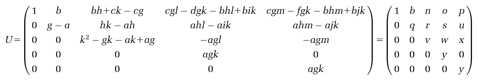
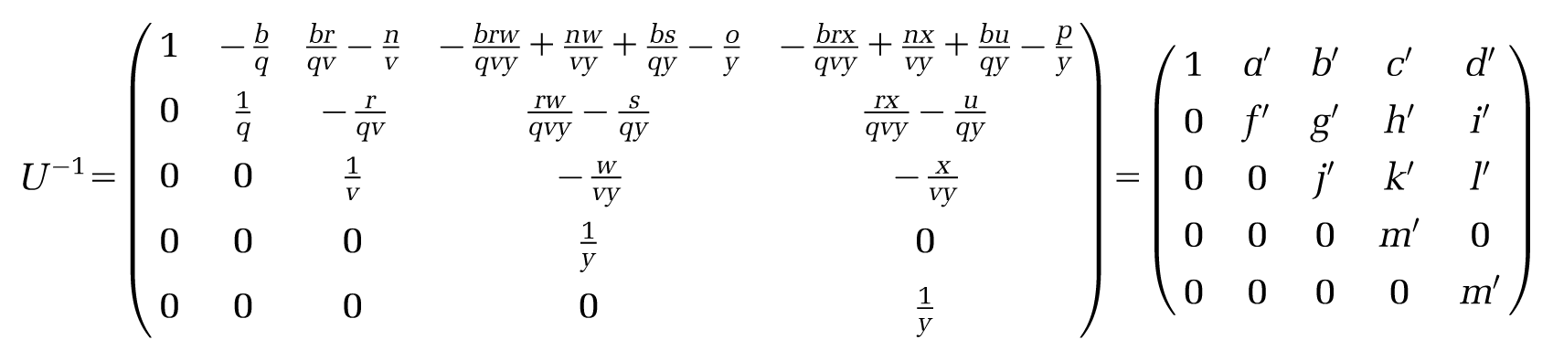
The paper illustrates the steps required to solve the Kolmogorov equations using the diagonalization approach. We show how to derive and apply algebraic formulas for the conversions that can be used for a wide variety of models with four or five states and some models with six or more states. The formulas use several sets of intermediate variables, so that the individual formulas are relatively simple and can be entered into an Excel spreadsheet, with one formula in each cell and no need for macros or Visual Basic. The mathematical methods themselves are not novel; the use of intermediate equations is really just a way of keeping the calculations tidy, and provides clarity for those who may not be familiar with the underlying mathematics.
Previous publications have given formulas for converting rates to probabilities for certain two- and three-state models3-5 and one four-state model. 4 For most models with larger numbers of states, the formulas are extremely complicated and these publications recommend numerical methods with software such as R (the msm package) or WinBUGS and WBDiff. This approach may be practical if one is willing and able to implement the entire model in R or WinBUGS—though many analysts are still more comfortable working with Excel, for example because they consider it easier or because it facilitates presentation of results to other stakeholders. In principle, WinBUGS can convert the rates to probabilities and produce samples from a probabilistic sensitivity analysis, which can then be saved and copied into a spreadsheet containing the decision model. However, this procedure might be unwieldy as it involves multiple software packages. Moreover, it is common for transition rates to vary according to an external measure of time, such as the age of the patient, which means that if numerical methods are used then the conversion from rates to probabilities has to be done for each age-group or cycle separately.
Our approach is aimed at analysts who develop decision models in spreadsheets, and should also be of interest to analysts who want to understand the mathematical derivation of the formulas used to convert rates to probabilities. The idea is that the analyst can set up the formulas once, and then copy them so that they are used for each age-group or cycle. Univariate sensitivity analysis and probabilistic sensitivity analysis are straightforward, as the direct connection from the rates and their standard errors to the transition probabilities is maintained and there is no need to copy and paste the samples from elsewhere. Another advantage is that this approach might be easier to audit and validate than an analysis where several software packages are used.
First we describe the mathematical background. Then we describe the usual procedure for deriving formulas to convert transition rates to probabilities, for models with forward and backward transitions. We illustrate this for a three-state model. We then discuss the situations in which the procedure does not work (it is easier to explain these after an example). Next we describe the new procedure with intermediate variables and illustrate it by examples with four- and five-state models. We also discuss how to derive the formulas using a computer algebra system instead of pen and paper. The final section is a discussion.
For all our example models, the formulas are set out in the accompanying Excel files (see supplementary material). For state-transition models of the appropriate structures, these files can be used directly. The analyst can simply copy the formulas into their own Excel files or copy their own transition rates into a copy of one of our Excel files. For models with other structures, the appropriate formulas will have to be derived using our procedure.
Kolmogorov’s Equations and the Matrix Exponential
Given the transition-rate matrix
In this paper we assume that
Here,
If
This is much simpler, since
Our formulas for the transition probabilities are based on this second formula for
There are several alternative terms and notations. Eigen-decomposition is sometimes known as spectral decomposition. If a matrix has an eigen-decomposition then it is said to be diagonalizable.
A Procedure for Deriving the Formulas When n is Small
For a given multistate Markov model, the formulas for
Step 1. Write down
Step 2. Derive formulas for the elements of
Step 3. Derive formulas for the elements of
Step 4. Derive formulas for the elements of
Step 5. Derive formulas for the elements of
Our presentation of this procedure is novel but mathematically these steps are closely based on the results in the previous section.
In Steps 2 and 3, the diagonal elements of
At each step, the formulas should be simplified using the standard rules of algebra. There are also several other ways of simplifying the formulas. Firstly, if the only possible transition from
If there are only forward transitions, then Step 2 is simple, because
The following is an illustration of the procedure.
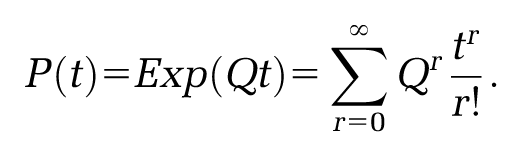
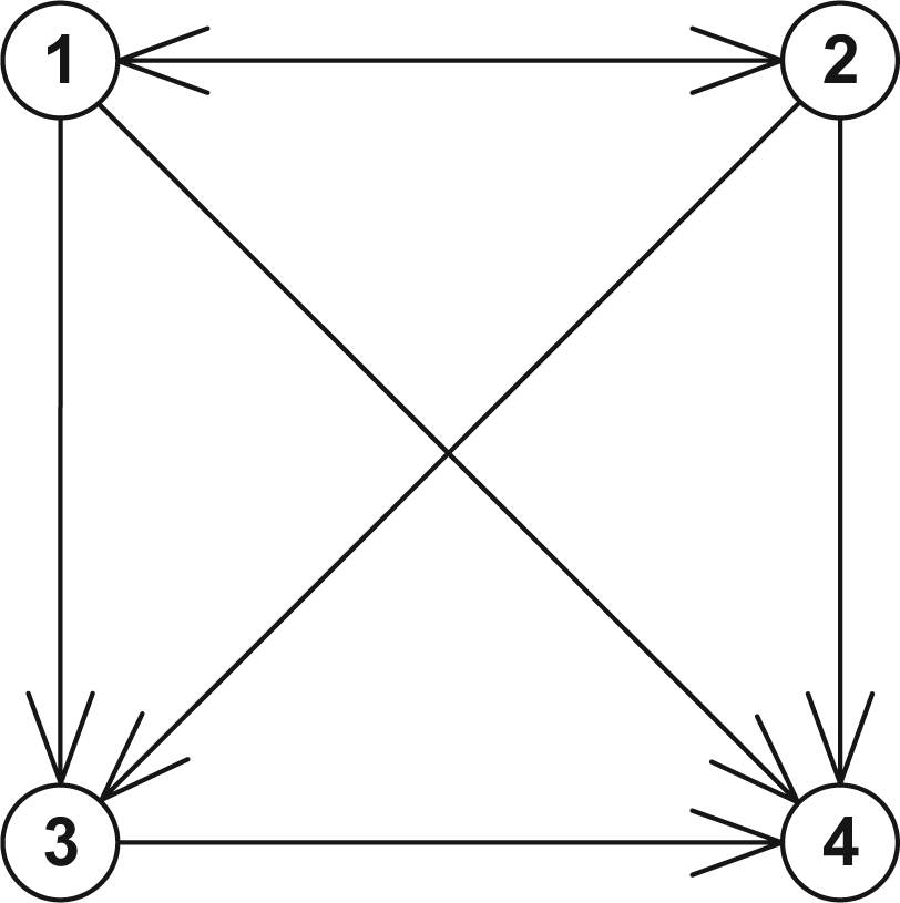
Model 1. Three-State Model with Forward Transitions Only (See Figure 1)
Step 1:
Step 2:
Step 3:
Step 4:
Step 5:
The final matrix here is equivalent to the final matrix in Figure 3 of Welton and Ades. 3 Formulas for the three-state model with all forward transitions and the backward transition from state 2 to state 1 have also been published. 4
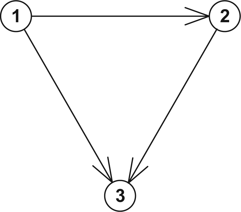
The states and transitions for Model 1, a three-state model with forward transitions only.
Situations Where the Procedure Fails
For some models with five or more states, especially ones with several backward transitions, it is impossible to find an algebraic solution of the characteristic equation (this follows from the Abel–Ruffini theorem
13
). Step 2 therefore fails. If this happens, it will be necessary to use the numerical methods mentioned in the introduction or calculate the matrix exponential
If the characteristic equation has an algebraic solution, then our method will usually work. But if two eigenvalues turn out to be exactly equal when numbers are put into the formulas, then it will fail. This is rare, because the rates are numbers on the continuous real line and it is unlikely that, for example, two of them will be exactly equal. But if it happens, then attempting to use the formulas will result in division by zero and the software will raise an error or give an output of infinity. This can happen either in Step 3, if the formulas for the eigenvectors involve division, or in Step 4, when the matrix is inverted.
Problems can also arise if two of the eigenvalues are very close to each other, or if certain other numbers are very close; if the difference of two such numbers appears in a denominator, then the result can be inaccurate (which other numbers this applies to depends on the model and how the formulas are written; for example, in Model 3
Lastly, if the model is beyond a certain size, then solving the characteristic equation algebraically may be possible in theory but too complicated in practice. These issues mean that output from the formulas should always be treated with caution. If the probabilities seem implausible then it will be necessary to calculate the matrix exponential by other methods as described above. For PSA it may also be worth making scatter plots of the final probabilities to check that they look plausible.
In some models the eigenvalues might be complex—that is, one or more of them involves the square root of a negative number. If this happens in Excel then there will be a #NUM! error, and the formulas will need to be rewritten using functions such as IMSQRT and IMSUM, but the procedure should still work. In our five example models, the eigenvectors are all always real.
A Procedure for Larger n, Using Intermediate Variables
In theory, the procedure described above works for any
Model 2. Four-State Model with Forward Transitions Only (See Figure 2)
Our work on this procedure arose from an empirical application for which this four-state model can be used. The four states are “healthy,”“had minor cardiovascular event,”“had major cardiovascular event,” and “dead.” The reason for having two cardiovascular disease states is that when a person has had a minor event they are more likely to go on to have a major event, and the mortality rate after a major event is greater than the mortality rate after a minor event.
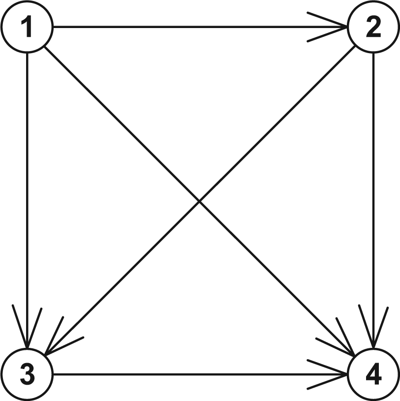
The states and transitions for Model 2, a four-state model with forward transitions only.
Single roman letters like
Step 1:
Step 2:
For this model, there is no need to introduce intermediate variables at this step.
Step 3: In this step,
As an illustration, the second column of
The intermediate variables are
Step 4: In this step,
As an illustration, the
The formulas for the new intermediate variables are
Step 5:
The formulas for the transition probabilities are
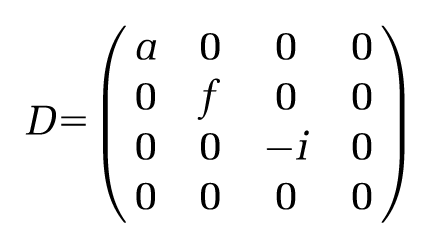
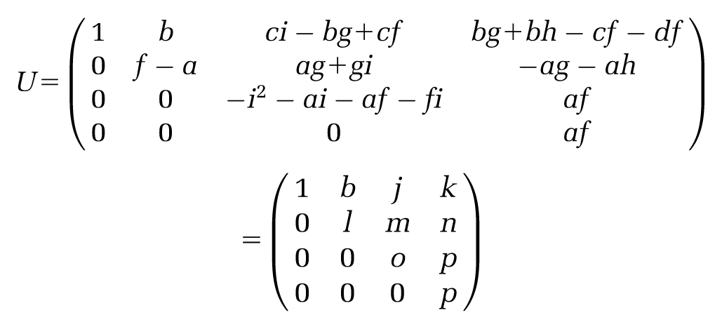
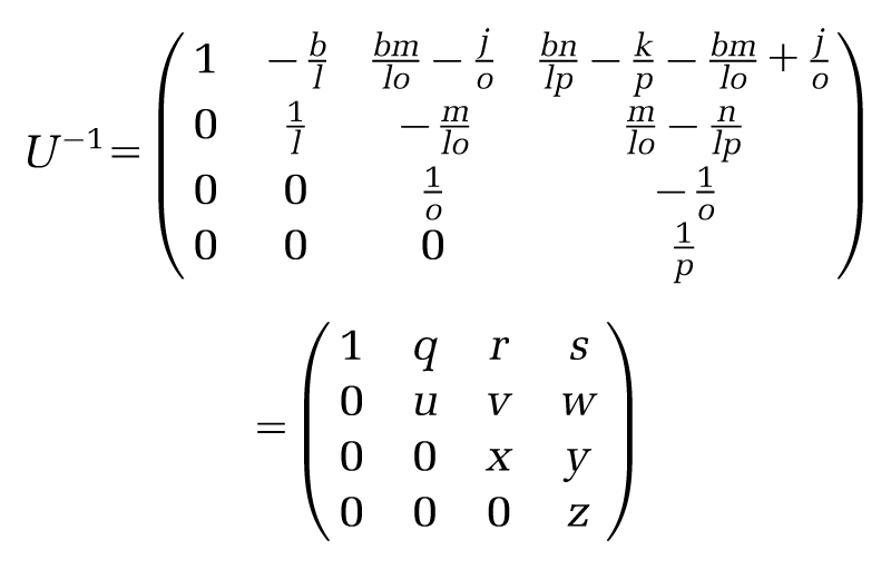
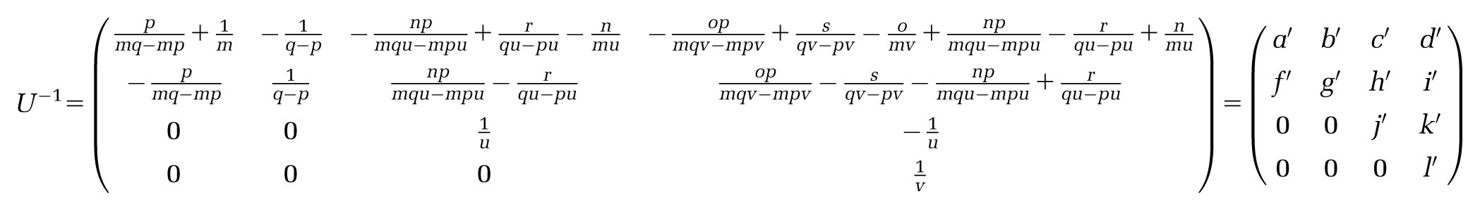
Model 3. Four-State Model with Forward Transitions and One Backward Transition (See Figure 3)
Step 1:
Step 2: The characteristic equation is
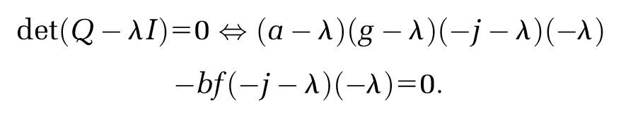
The solutions
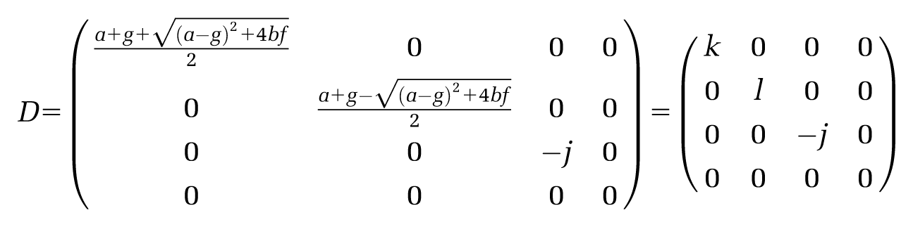
The intermediate variables here are
Step 3:
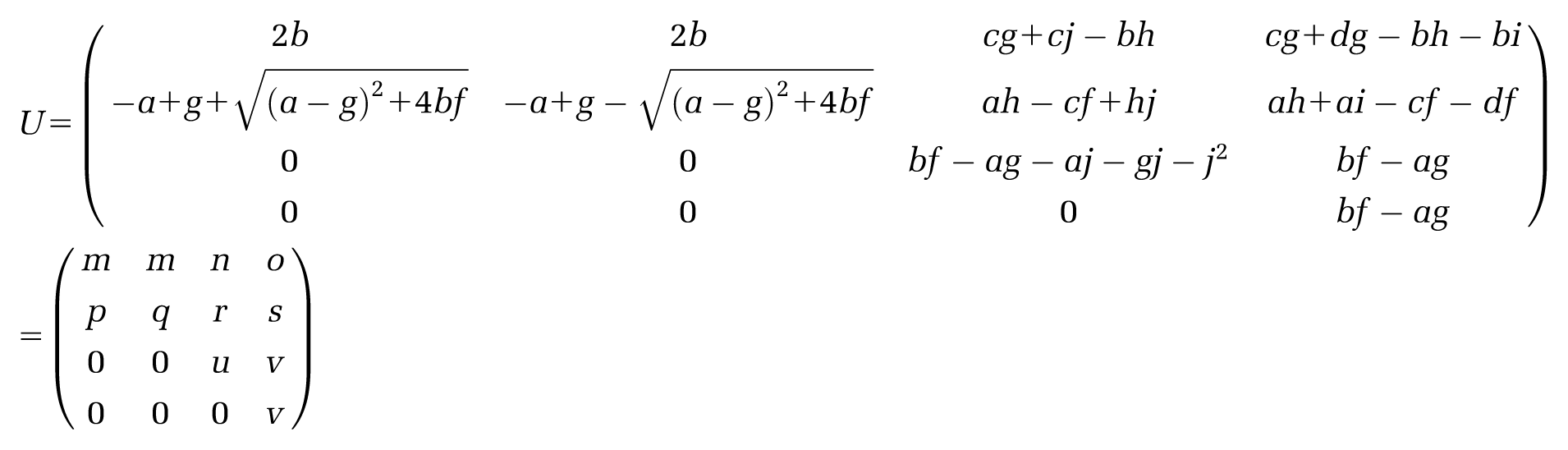
This time
Step 4:
Step 5:
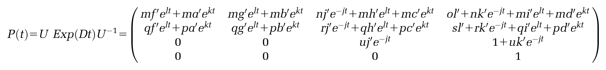
The states and transitions for Model 3, a four-state model with forward transitions and one backward transition.
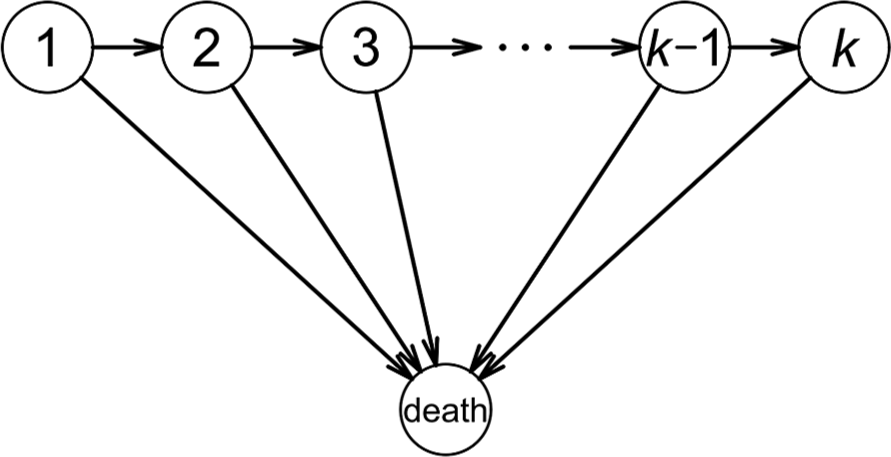
Model 4. Five-State Model with Forward Transitions Only and Two Death States (See Figure 4)
Step 1:
Step 2:
Step 3:
The formulas for the intermediate variables in
Step 4:
The formulas for the intermediate variables in
Step 5:

The states and transitions for Model 4, a five-state model with forward transitions only and two death states.
The formulas created by this procedure are suitable for working in Excel with one cell at a time. Each set of numbers or formulas can be arranged in the form of a matrix, and these matrices can be placed next to each other, for example in the order
The main reason why using intermediate variables is preferable to using a single set of direct formulas is that the formulas are much simpler. They are also easier to understand and organize because they correspond exactly to the matrices and equations for the solution to Kolmogorov’s equations. The disadvantage is that it involves more formulas.
The idea of using intermediate variables to simplify formulas for transition probabilities has been used in the field of applied biostatistics. See for example section 4.2 of Chiang, 23 which is about models in which there are two alive states, with transitions both ways between them, and an arbitrary number of death states. Intermediate variables are used for the two non-zero eigenvalues.
Using a Computer Algebra System
The four sets of formulas described in the previous sections are derived by eigen-decomposition, matrix inversion, and matrix multiplication. These derivations can all be done using pen and paper but it may be easier and more reliable to use a computer algebra system (CAS). The best-known CASs are Maple, Mathematica, and Matlab. In Matlab, the functions “eig” and “inv” can be used to find
There are various free CASs but not all of them have the necessary capabilities for deriving the formulas. One that does is Maxima.
24
The code below shows what a user might type in Maxima to work out the formulas for Model 2 as shown above. The code is not a template that can be adapted to other models by simple changes like replacing zeroes with letters. Instead, after each step it is necessary to look at the output and decide what to type next. Maxima does not necessarily give the formulas in their simplest possible forms, so there is a need for judgement and trial and error in deciding how to define
If Step 2 involves solving a cubic or quartic equation, then that is likely to be slow even with a CAS, and of course if there are several backward transitions and no algebraic solution, then a CAS will not be able to get around this problem.
Model 2. Four-State Model with Forward Transitions Only
Probably the easiest way to use Maxima is wxMaxima, which has a graphical interface. One setting that may be useful is: Edit – Configure – Enter evaluates cells. For simplifying, useful functions are “expand” and “ratsimp”.
Discussion
For any given model, the four sets of formulas can be worked out by hand or by using a CAS, so long as the characteristic equation has an algebraic solution. Because the eigenvectors can be multiplied by constants, there are countless different possibilities for the formulas, but when the formulas are used on numerical transition rates, the results should be the same.
There is a rich variety of multistate Markov models with
The disease progression model.
An analyst who is familiar with R would probably prefer to develop the entire decision model in R, using a package such as expm to calculate the matrix exponential. However, many analysts still prefer to develop decision models in spreadsheets, and this paper is aimed at them. In the case where a decision model has been developed in a spreadsheet, the current alternative to our approach for calculating probabilities from rates would be to calculate the matrix exponential using an external package such as R or WBDiff and copy and paste the results into the spreadsheet.
An advantage of our algebraic formulas for the transition probabilities over numerical methods such as WBDiff is the speed and simplicity of running the calculations multiple times for probabilistic sensitivity analyses. PSA enables calculation of the overall probability that a treatment is more effective or cost-effective than another, based on all the information in the model, and serves also as the basis for expected value of information (EVI) analyses.
As mentioned in the introduction, the “simple formula” is sometimes used instead to convert from transition rates to probabilities:
The question arises of when the simple formula might be approximately correct and sufficient for practical purposes. This happens when all the rates of transitions from
Footnotes
Acknowledgements
This paper was inspired by conversations that Neil Hawkins and Alex Sutton had with David Epstein in 2011. The authors would like to thank Simon Thompson and Stephen Kaptoge for their helpful comments. They would also like to thank Laura Vallejo-Torres for her thoughtful presentation and discussion about this paper at the Health Economists’ Study Group in June 2016.
This work was performed at the Department of Public Health and Primary Care, University of Cambridge; Departamento de Economía Aplicada, Universidad de Granada; Escuela Andaluza de Salud Pública, Campus Universitario de Cartuja.
Financial support for this study was provided in part by grants from the UK Medical Research Council (G0800270), British Heart Foundation (SP/09/002), UK National Institute for Health Research Cambridge Biomedical Research Centre, European Research Council (268834), and European Commission Framework Programme 7 (HEALTH-F2-2012-279233). This work was financially supported by the EPIC-CVD project. EPIC-CVD is a European Commission funded project under the Health theme of the Seventh Framework Programme, building on EPIC-Heart, which was funded by the Medical Research Council, the British Heart Foundation, and a European Research Council Advanced Investigator Award. The funding agreements ensured the authors’ independence in designing the study, interpreting the data, writing, and publishing the report.
References
Supplementary Material
Please find the following supplemental material available below.
For Open Access articles published under a Creative Commons License, all supplemental material carries the same license as the article it is associated with.
For non-Open Access articles published, all supplemental material carries a non-exclusive license, and permission requests for re-use of supplemental material or any part of supplemental material shall be sent directly to the copyright owner as specified in the copyright notice associated with the article.