
Abstract
We propose a novel Bayesian model framework for discrete ordinal and count data based on conditional transformations of the responses. The conditional transformation function is estimated from the data in conjunction with an a priori chosen reference distribution. For count responses, the resulting transformation model is novel in the sense that it is a Bayesian fully parametric yet distribution-free approach that can additionally account for excess zeros with additive transformation function specifications. For ordinal categoric responses, our cumulative link transformation model allows the inclusion of linear and non-linear covariate effects that can additionally be made category-specific, resulting in (non-)proportional odds or hazards models and more, depending on the choice of the reference distribution. Inference is conducted by a generic modular Markov chain Monte Carlo algorithm where multivariate Gaussian priors enforce specific properties such as smoothness on the functional effects. To illustrate the versatility of Bayesian discrete conditional transformation models, applications to counts of patent citations in the presence of excess zeros and on treating forest health categories in a discrete partial proportional odds model are presented.
Keywords
Introduction
Discrete data commonly occur in almost every scientific area. In this article, we focus on the two relevant cases of count data and ordinal data as special instances of discrete response structures. Before the advent of generalized linear models (GLM, Nelder and Wedderburn, 1972), the peculiarities of count data were either ignored or treated simply by log transformations (Sokal and Rohlf, 1981). Then, the standard modeling approach for count data Y ∈ {0, 1, 2,…} became Poisson regression,
Similar to counts, ordered categorical data Y ∈ {1,…, c + 1} occur in a manifold of scientific disciplines such as medicine or the social sciences. A researcher in medicine, for example, may want to distinguish between different kinds of infection grades, while an ecologist could be interested in measuring forest health in terms of defoliation categories. Exploiting the natural ordering in these kinds of data is firmly established in the statistical community by cumulative link models as shown in McCullagh (1980). Prominent versions are the discrete proportional odds model and the discrete proportional hazards model (Tutz, 2011). In its simplest form, the cumulative link model is given by
The dissemination of Markov chain Monte Carlo (MCMC) simulation techniques led to the development of Bayesian analogues for established models in the form of Bayesian GLMs (Dey et al., 2000) with many extensions, for example, by Friihwirth-Schnatter and Wagner (2006), Fruhwirth-Schnatter et al. (2009), Rodrigues (2003) and the Bayesian GAM (Brezger and Lang, 2006). Ghosh et al. (2006) describe a Bayesian treatment of zero-inflated regression models, and Klein et al. (2015a) introduce zero-inflated and overdispersed count data to the framework of Bayesian structured additive distributional regression (Klein et al., 2015b). In a non-transformation environment, Lavine and Mockus (1995) and Dunson (2005), among others, apply a (strictly) isotonic regression function for count responses on the basis of a Dirichlet process mixture prior.
To bridge the gap between discrete ordinal and count regression models, we consider count data as ordinal categorical data with a very high number of intercept thresholds that, however, are not estimated but rather are fixed by design at all non-negative integers. Methodologically, both approaches are unified by the idea of a direct parametrization of the transformation function. Similar to Siegfried and Hothorn (2020), we treat the smooth parametrization of the thresholds as the defining element of the count transformation approach used in this article. While overdispersion is absorbed by the smooth transformation of the counts, we supplement the model with a second component that explicitly accounts for eventual zero inflation. For a discussion of the connection between (binary) regression and transformation models, see Doksum and Gasko (1990).
To summarize, in this article, we aim to do the following:
Propose a Bayesian approach for count transformation models based on flexible transformation functions that are inferred from the data, which-in its simplest form with linear covariate shift effects-results in a distribution-free yet interpretable model framework for count data that automatically accounts for over- and underdispersion in the response distribution, Account for excess zeros in two-component mixtures models, Propose a Bayesian approach for cumulative link transformation models with Bayesian proportional odds and proportional hazards models as special cases, Allow for the inclusion of category-specific effects, resulting in non-proportional transformation model types, Combine both model types into the class of Bayesian discrete conditional transformation models (BDCTM) and establish it as an extension of Bayesian conditional transformation models (BCTM) for continuous responses, Supplement all models with non-linear, possibly high-dimensional covariate effects and interactions, and Illustrate BDCTM's capability in the presence of count and categoric data in two applications.
The rest of this article is structured as follows: Section 2 introduces the model class we refer to as BDCTM with a preliminary discussion of its building blocks. Section 3 contains a description of posterior estimation. A simulation study evaluating BDCTM's performance in a count data setting is presented in Section 4. Section 5 features an application on patent citation counts and an application on forest health categories. We conclude in Section 6.
Bayesian discrete conditional transformation models
In what follows, we introduce BDCTM as a model class that represents a novel approach to the direct estimation of the conditional distribution function
Let y be an observation of a count or ordered categorical response variable Y and let

The responses are transformed towards the reference distribution conditionally on
We proceed with discussing each of the components ofa BDCTM in more detail. Section 2.1 introduces the basic structure assumed for the transformation functions. Sections 2.2 and 2.3 present model variants for count data and ordinal responses, respectively, while Section 2.4 discusses a generic basis function representation for the transformation functions. Section 2.5 introduces the corresponding prior assumptions, Section 2.6 discusses partial contributions to the transformation function, and Section 2.7 contemplates on the relevance of the choice of the reference distribution.
Similar to Hothorn et al. (2014), we assume an additive decomposition on the scale of the transformation function into J partial transformation functions
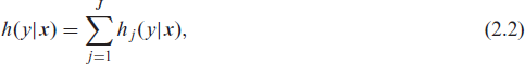
where hj(y|

where in
We distinguish between two related model types for count data: simple shift count transformation models that are able to deal with overdispersion and two-component mixture transformation models that can additionally deal with excess zeros.
Mean-shift count transformation models: Regular count transformation models are defined by shifts of the non-linear baseline transformation function hY:

where
Two-component mixture count transformation models: Besides over- and underdispersion, count data often come with an excess number of zeros, which needs to be accomodated in the model. One possibility is to add a second component to the linear transformation function that captures zeros (Hothorn et al., 2018). A transformation function in that vein can be depicted as:

where

The process generating non-zeros in this case is not explicitly truncated but stems from a transformation function that excludes the zeros.
All count transformation functions of this type have in common that they act on the floor function
For ordered categorical data, we distinguish between cumulative models with and without categoryspecific shifts. From a transformation perspective, the latter are modeled in terms of response- covariate interactions that can be linear or non-linear in direction of the respective covariate.
Proportional models: The simplest cumulative transformation model is:

where the term h(
Non-proportional models: Models of type (2.7) can be generalized by a category-specific shift resulting in the following model:

where hr (
We assume that each of the J partial transformation functions can be approximated by a linear combination of basis functions
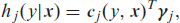
where γj is a vector of basis coefficients. Based on the additivity assumption in (2.2), the complete conditional transformation function can be denoted as

with joint basis

and

This allows us to write all discrete conditional transformation models treated in this article in the general form:

We call models of type (2.11) Bayesian discrete transformation models (BDCTM). They can be conceived as extensions of the versatile model class of BCTM for continuous responses that were introduced by Carlan et al. (2020), taking the additional challenges arising from discrete responses into account. In this tradition, a BDCTM is fully specified by a reference distribution FZ, the joint basis
Let

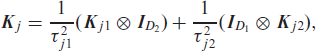
where
where the Kronecker product forms parametric interactions between the evaluated basis functions, and
We require all transformation functions to be strictly monotonically increasing solely in the direction of y but not in direction of the explanatory variables such that

and
The vector of basis coefficients for the whole conditional transformation function h(y|
Of course, other basis specification could be employed to set up BDCTMs, as long as monotonicity along y is ensured. For example, the increasing splines considered in continuous ordinal regression (Manuguerra and Heller, 2010) would be a potential alternative. We rely on Bayesian P- splines and their tensor product interactions since these have been extensively studied in Bayesian structured additive regression and enable efficient and stable computations.
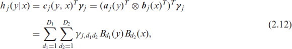
We adopt the principle of Bayesian P-splines (Lang and Brezger, 2004) and assume partially improper multivariate Gaussian priors for the unconstrained vectors βj1 and βj2 (the reparameterized vectors γj1 and γj2 are based on) such that
where
where precision matrices
The smoothing variances
We start this section by introducing the two types of basis functions we use in
Smooth basis for count transformations: In case of a count response
Discrete basis for ordinal categorical data For ordered categorical responses,

The corresponding precision matrix is
Bases for covariates effects For covariate effects we allow linear bases
Transformation random effects hj (x) = βg are based on the grouping indicator g ∈ {1,…, G}. The corresponding G-dimensional basis vector
In the context of discrete conditional transformation models, the reference distribution function FZ plays the role of the inverse link function controlling the interpretational scale of the impact of the explanatory variables. While it can be chosen arbitrarily in theory, we concentrate on distributions with log-concave densities for FZ to guarantee uniqueness of the maximum likelihood estimate, which usually will also imply unimodality of the posterior. Furthermore, it is advised to consider characteristics such as right-skewness or the support of the count data distribution in the selection process. Prominent choices for FZ are
FSL(z) = (1 + exp(-z))−1, that is, the standard logistic distribution, FMEV(z) = 1 - exp(- exp(z)), that is, the minimum extreme value distribution
This results in logit, probit or cloglog interpretations of the covariate effects. Setting FZ = FSL, for example, results in the discrete proportional odds model and FZ = FMEV results in the proportional hazards model, with h(
To reflect specific properties of the data-generating process, other link functions that have been considered in the context of GLM, such as skew-logistic or t-distributed link functions to reflect strong asymmetry or heavy tails, may be considered. However, given the flexibility of the transformation function, we do not expect large gains from such specifications since both asymmetry and tail behaviour should be taken up by the transformation function, leaving only a small potential for improving the fit via the link function. We therefore suggest to stick to the defaults and to select the reference distribution according to preferences on model interpretation.
Transformation probability mass functions
In this section, we introduce the transformation probability mass functions (PMFs) resulting from the different sampling assumptions that come with count and ordinal categoric data as well as the resulting transformation likelihoods. To emphasize that

In case of an ordinal categorical response with bounded support Y ∈ {y1,…, yc+1}, the corresponding conditional distribution function needs to take the additional constraint for the reference category c + 1,
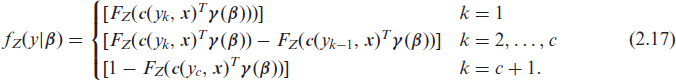
With the convention

encompassing count and ordered categoric models in a unified framework (Hothorn et al., 2018). Based on (2.18), the transformation log-likelihood for independent observations (yi,
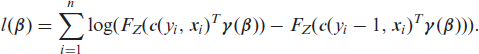
The likelihood is chosen according to the discrete response structure only, while the transformation function determines whether excess zeros are accounted for or if the category-specific effects are included, for example. With all building blocks in mind, a BDCTM can be fully specified by the set
For Bayesian inference, we rely on MCMC simulation techniques. We sketch the most relevant parts of the algorithm in this section.
Update of the basis coefficients: The log-full conditional of the basis coefficients (up to an additive constant) is given by
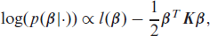
where the second term arises from the multivariate Gaussian prior. The gradient of the unnormalized log-posterior is needed for inference and is given by

where
Strong dependencies among the variables (which are partly due to the monotonicity restriction) complicate the sampling from the posterior distribution. This is further impeded by the mixed linear- non-linear dependence of the transformation function on
Update of the smoothing variances: In the univariate case, updating the smoothing variance is straightforward by using the full-conditional:
where

we need to consider the generalized determinant of (3.1) when updating the smoothing variances. This aggravates sampling, which is why we introduce an anisotropy parameter
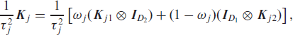
where ωj controls how much prior information is assigned to each of the two covariates of the tensor spline. For the BDCTM, we consider a discrete prior for ωj, which allows to pre-compute a finite set of generalized determinants that can be used within the MCMC simulations (see Kneib et al., 2019) for a detailed explanation of this approach).
In the following, the hyperparameters of the inverse gamma prior are set to aj1 = aj2 = 1, bj2 = bj2 = 0.001, resulting in good and stable performance in all investigated cases.
Numerical stability: Klein et al. (2015a) observed numerical problems if zero-inflation was wrongfully assumed when in fact, for example, a simple Poisson model was due. One reason is that the estimated predictor for the probability of an extra zero tends towards minus infinity in log-space. This is usually not an issue in models of type (2.5) as the coefficients that are related to the zero component are not exp-transformed. In cumulative models with category-specific effects, however, flat sections can lead to divergent transitions in which case weakly identified coefficients have to be dropped from the model (Pya and Wood, 2015). This issue can be remedied by adding
Software: All computations were carried out in R version 4.1.0 (R Core Team, 2020). To improve computation time, likelihoods and score functions were implemented via the package
In this section, we present a simulation experiment that highlights the possible advantages of the count transformation approach in general and that compares our Bayesian approach with the likelihood-based linear count transformation model by Siegfried and Hothorn (2020).
Count transformation models can mimic most well-known models for count data. Therefore, a meaningful simulation study in this setting needs to consider the sensitivity of the flexible transformation function with respect to the true data-generating process. In other words, it needs to investigate to what extent the flexible transformation function is able to accommodate eventual overdispersion and other characteristics of possibly complex data generating processes.
Simulation design: We use a similar simulation design to Siegfried and Hothorn (2020) with the following properties:
One covariate is generated via Conditional on z, we consider five different count data generating processes (DGPs)
Poisson with mean and variance Negative Binomial with Three different count data-generating processes according to Each dataset was estimated by their corresponding true (oracle) models, that is, a Poisson GLM (mp), a negative binomial GLM (mnb), BDCTMs (bmlo denotes the logistic model, bmpr denotes the probit model and bmcll denotes the cloglog model) and a frequentist count transformation model (Siegfried and Hothorn, 2020) implemented in the Training and validation sample sizes are set to 250 and 750, respectively. The simulation experiment was repeated in 100 replications with a total iteration number of 2,000 and a burn-in and warm-up phase of length 1,000, such that 1,000 iterations are being used for computing the estimates.
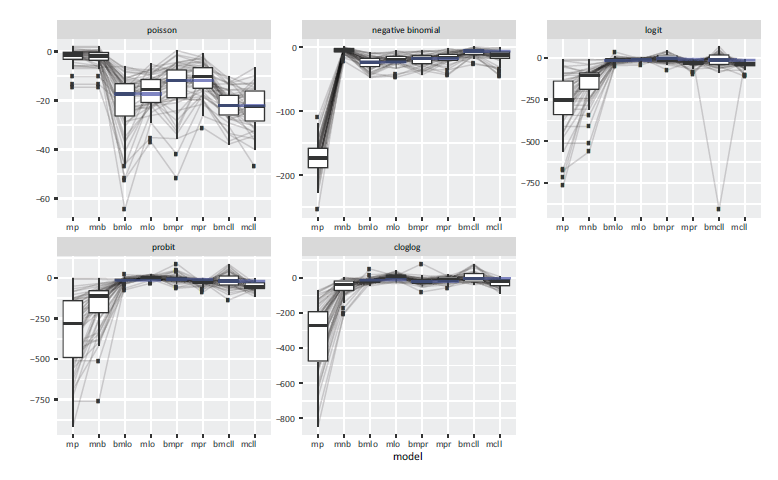
Each model fit is quantified by means of the centered out-of-sample log-likelihood resulting from the difference between the out-of-sample log-likelihoods of the models and the out-of-sample loglikelihoods of the true data-generating processes evaluated on a hold-out sample, taking a predictive perspective that implicitly controls for differenes in complexity between the models. The results presented in Figure 1 confirm most of the findings of Siegfried and Hothorn (2020) regarding the merits of the count transformation approach.
Comparison of count data-generating processes on basis of centered out-of-sample log-likelihoods obtained from the respective model. Larger out-of-sample log-likelihoods indicate a better performance of the corresponding model.
Based on these results, we can make the following statements:
The Poisson model, being the most rigid model, shows the worst performance with respect to the out-of-sample log-likelihood, if misspecified. As expected, the negative binomial model performs well for the Poisson and the overdispersed case, but shows inferior performance in the remaining scenarios. The fit of both the BDCTM and the The BDCTM seems to perform better than
The simulation study confirms the robustness of the BDCTM in the presence of different data- generating processes. Its fit is satisfactory in all investigated cases and highly competitive in the more complicated scenarios. While the Poisson distribution only works well in simple scenarios, the negative binomial distribution also works quite well for most scenarios (except the Poisson case). Still, BDCTMs outperform negative binomial regression uniformly over all but the Poisson and the negative binomial scenario.
We illustrate possible applications of the BDCTM in this section. For better readability, we add the number of basis functions to the basis, for
Patent citations with excess zeros
Similar to an author of a scientific publication, an inventor who applies for a patent has to cite all existing patents their work is based on. We analyze the citation number (ncit : y) of patents granted by the European Patent Office (EPO). The considered dataset includes five dummys and three continuous variables. The available continuous covariates are the grant year (year), the number of the designated states (ncountry) and the number of patent claims (nclaims). (For a full description of the explanatory variables in the data set of n = 4,805 observations, see Jerak and Wagner 2006). A high rate of zeros (≈ 46%) and a big spread ncit ∈ {0,…, 40} hint on the presence of zero-inflation and overdispersion. A rigorous investigation of this presumption has to consider whether this is holds conditional on the covariates. We let the sampler run for 2,000 iterations with a burn-in and warm-up phase of length 1,000 such that 1,000 iterations are obtained for inference.
We start our investigation with the simple linear transformation model (BDCTMlin):

where the linear predictor
Patent citations. Rootograms of the linear Poisson, the linear negative binomial and the simple linear BDCTM model.
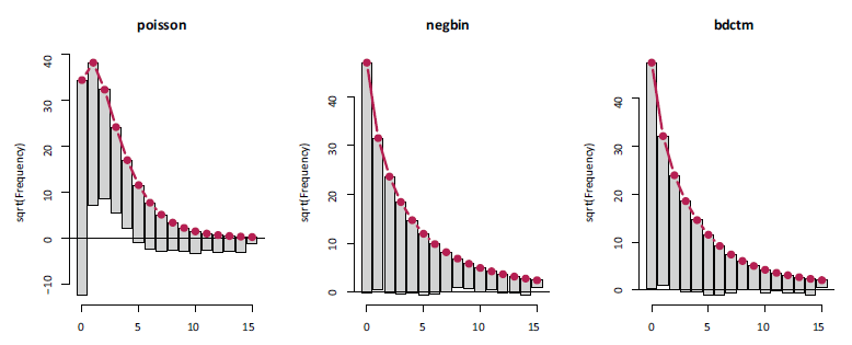
In summary, this first visual inspection of the goodness-of-fit confirms that BDCTM is able to ameliorate the impact of overdispersion on the model fit.
We also want to pursue the assumption of excess zeros. For this, we consider a two-component model (BDCTMhurdle-lin) in the vein of (2.5) with

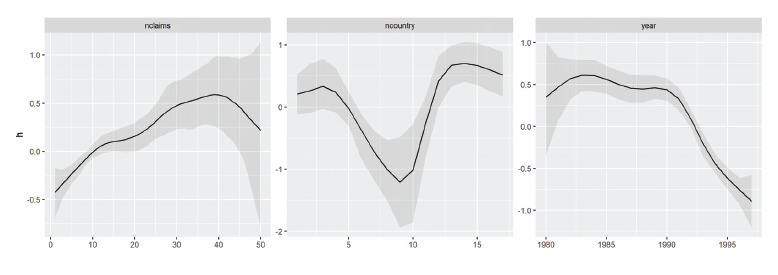
where, again,
Patent citations. Posterior mean estimates of the effects of nclaims, ncountry and year on the log-odds ratio, together with 95% credible intervals. Remaining covariates are held constant at their mean or are set to zero in case of dummy variables. Estimates belong to BDCTMnl.
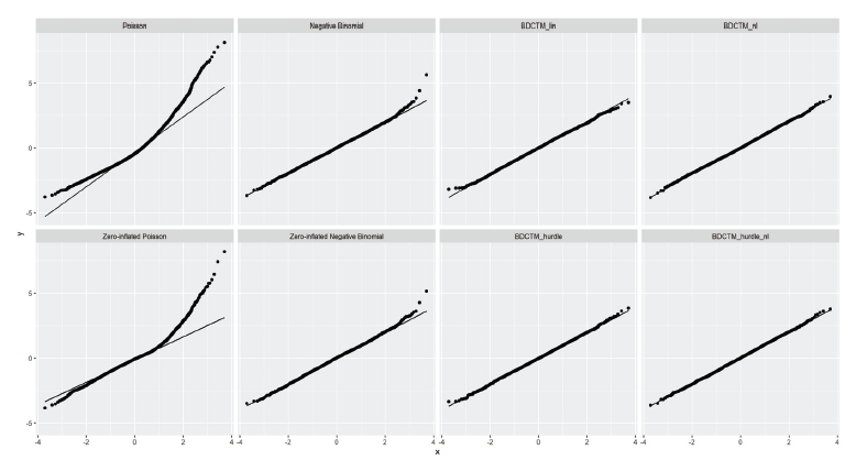
In the next step, we compared all models in terms of randomized quantile residuals as proposed by Rigby et al. (2008). For every observation yi, we computed residuals
Patent citations. Comparison of quantile residuals obtained by BDCTM models with and without addititional zero component with various generalized linear and zero-inflated models.
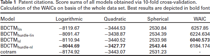
For a more rigorous assessment of the out-of-sample performance, we conclude our analysis with an evaluation based on proper scoring rules. Originally proposed by Gneiting and Raftery (2007), they serve as summary measures for the predictive power of a model. Based on data y1, …, yR in a validation sample and estimated probabilities Brier score: Logarithmic score: Spherical score:
The probabilistic forecasts collected in
Patent citations. Score sums of all models obtained via 10-fold cross-validation. Calculation of the WAICs on basis of the whole data set. Best results are depicted in bold font
This short analysis involving non-linear category-specific effects is based on data from the forest of Rothenbuch (Spessart) over the years 1982-2004. Every year, the health status is evaluated and categorized by the response variable defol measuring defoliation grades. Since data is sparse in some of the original nine categories (0%, 12.5%, …, 100%), we aggregated them into the three defoliation grades: 1 = no (0%), 2 = weak (12.5% - 37.5%) and 3 = severe (≥ 50%). Among others, the dataset comes with the covariates canopy (canopy density in percentage), x, y (x- and y-coordinates of location) and id (tree location identification number.). (Check Fahrmeir et al. (2013) for a full description of the dataset). The goal of this analysis is to determine the effect of the covariates on the degree of defoliation. Since the forest data is notorious for confounding and high autocorrelation, we let the sampler run for 10,000 iterations with a burn-in and warm-up phase of length 1000.
For this, we set up the partial proportional odds model
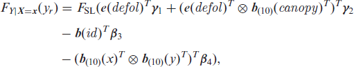
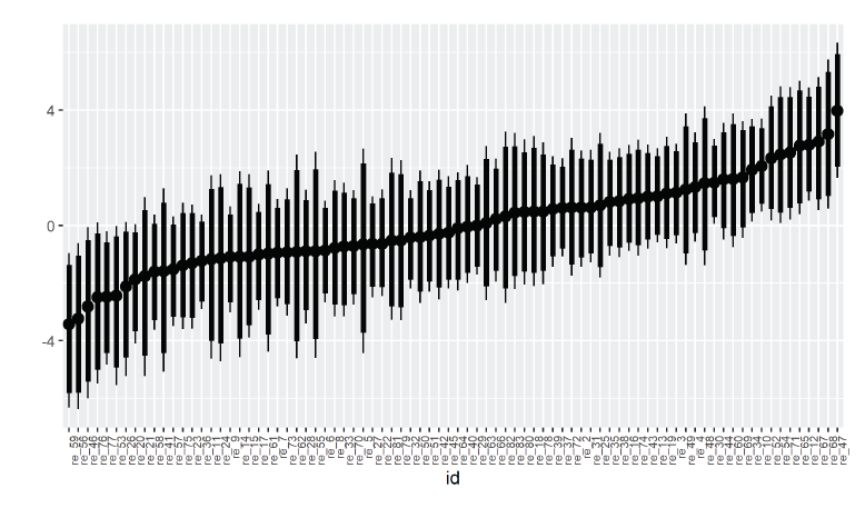
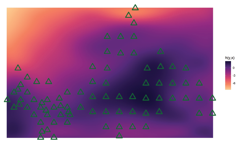
where we assume non-linear category-specific shifts of canopy, a transformation random effect for the tree location groups and a spatial non-linear effect on the basis of a tensor spline for the coordinates x and y. Figure 5 shows the estimated non-linear category-specific effect for canopy. The section for 0 ≤ canopy ≤ 25 displays almost parallel curves, which then vary more and more individually until they even cross. The variance of the estimated random effect for id is 2.42, and the standard deviation is 1.55. Figure 6 shows the estimated random intercepts. In a preliminary run, we observed the same problems with confounding in location-specific effects as Fahrmeir et al. (2013), which could be improved to some extend by adding the spatial effect. It is displayed in Figure 7.
Forest health: estimated non-linear category-specific effect of canopy, “no defoliation” in red, “severe defoliation” in blue, together with 95%-credible intervals.
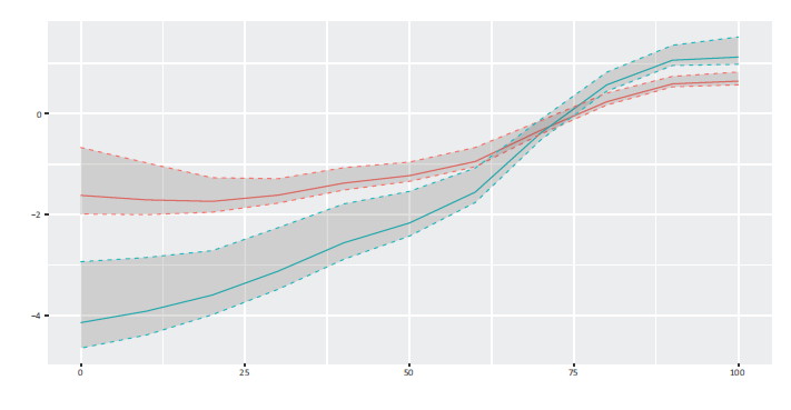
Forest health: estimated non-linear category-specific effect of canopy, “no defoliation” in red, “severe defoliation” in blue, together with 95%-credible intervals.
Forest health: median-sorted estimated random intercepts for tree location groups.
Forest health: estimated two-dimensional spatial effect with triangles indicating observed tree locations based on 2nd order penalties.
With the BDCTM, we present a novel Bayesian model framework for discrete data that combines cumulative link models with models for count data through directly modeling the conditional distribution function. Approaching these discrete data structures from the transformation perspective allows us to unify models that are usually treated seperately under the same umbrella. The BDCTM is flexible in the sense that it permits the user to control interpretability by means of choosing a reference distribution in conjunction with an additive transformation function. Estimating the conditional distribution function directly makes deriving distributional aspects such as the conditional quantiles straightforward by numerical inversion of FZ(h(y|
We demonstrate BDCTM's ability to handle under- or overdispersion in an adaptive fashion without restrictive distributional assumptions in Sections 4 and 5. A short investigation of a nonlinear non-proportional odds model highlights the versatility of our approach. In a model selection context, the unifying scope of the transformation function turns out to be a valuable simplification because there is just one “predictor” that has to be constructed. Though not shown in this article, it is possible to establish a relationship between overdispersion and the covariate effects by including full non-linear interactions between the count response and the respective explanatory variable. Constructing the conditional transformation function can be difficult as informed decisions about which effects to include and to interact with the response are required. Therefore, it would be desirable to develop an effect selection strategy via spike and slab priors in the spirit of Klein et al. (2021) for the BDCTM that could effectively tell the user what kind of effect is impacting the regular count process, the zero component or overdispersion.
As demonstrated in Section 5.2, our cumulative link transformation approach can be supplemented with category-specific linear or non-linear effects by modeling them as response-covariate interactions. This way, popular models such as (non-)proportional odds or hazards models can be retrieved simply by specifying the reference distribution. Both the count and the ordinal model could be supplemented with a more flexible link function as proposed by Aranda-Ordaz (1983), that is,

which depends on an auxiliary parameter
To conclude, we believe that in this article, the BDCTM is established as a flexible, modular modeling framework in the world of discrete data that is competitive in many modern scenarios.
Supplementary material
Supplementary material is available online.
Supplemental Material for Bayesian discrete conditional transformation models by Manuel Carlan, Thomas Kneib, in Statistical Modelling
Footnotes
Declaration of conflicting interests
The authors declared no potential conflicts of interest with respect to the research, authorship and/or publication of this article.
Funding
Thomas Kneib received financial support from the DFG within the research project KN 922/9-1. The work of Manuel Carlan was supported by DFG via the research training group 1644.
Note
References
Supplementary Material
Please find the following supplemental material available below.
For Open Access articles published under a Creative Commons License, all supplemental material carries the same license as the article it is associated with.
For non-Open Access articles published, all supplemental material carries a non-exclusive license, and permission requests for re-use of supplemental material or any part of supplemental material shall be sent directly to the copyright owner as specified in the copyright notice associated with the article.