
Abstract
Continuous-time state-space models (SSMs) are flexible tools for analysing irregularly sampled sequential observations that are driven by an underlying state process. Corresponding applications typically involve restrictive assumptions concerning linearity and Gaussianity to facilitate inference on the model parameters via the Kalman filter. In this contribution, we provide a general continuous-time SSM framework, allowing both the observation and the state process to be non-linear and non-Gaussian. Statistical inference is carried out by maximum approximate likelihood estimation, where multiple numerical integration within the likelihood evaluation is performed via a fine discretization of the state process. The corresponding reframing of the SSM as a continuous-time hidden Markov model, with structured state transitions, enables us to apply the associated efficient algorithms for parameter estimation and state decoding. We illustrate the modelling approach in a case study using data from a longitudinal study on delinquent behaviour of adolescents in Germany, revealing temporal persistence in the deviation of an individual's delinquency level from the population mean.
Keywords
Introduction
State-space models (SSMs) are flexible tools for analysing sequential observations that depend on underlying non-observable states, with interest and hence inference typically centred on the states. There are two main conceptual decisions to be made when tailoring an SSM to any given application, concerning (a) the nature of the state space and (b) whether the state process is defined as operating in discrete or continuous time. Regarding (a), the nature of the state space depends on the interpretation of the latent variable. The latter could relate either to discrete states, for example indicating an individual's health status (e.g., infected versus not infected; Conn and Cooch (2009) or an animal's behavioural modes (e.g., travelling, resting, and foraging; van Beest et al., (2019), or to continuous states, for example related to the nervousness of the financial market (e.g., within stochastic volatility models; Kim et al., (1998) or to an athlete's current form (e.g., in analyses of serial correlation in performance; Ötting et al., (2020). In some applications, the specification of the state space is obvious (e.g., in simple capture-recapture studies, with states corresponding to dead and alive; King and Langrock (2016), whereas in others it constitutes a modelling choice (e.g., in stochastic volatility modelling, where the market states are commonly considered to be continuous, but sometimes dichotomized to calm and nervous, respectively; Bulla and Bulla (2006). Regarding (b), that is, the decision whether the model is defined as operating in discrete or continuous time, the time formulation is usually determined by the sampling scheme of the data at hand. While discrete-time models are appropriate for time series with regular time intervals, continuous-time models are more suitable for irregularly spaced observations. However, as irregularly sampled data can often be augmented via imputation to give a regular series, or temporarily aggregated to yield regularly spaced observations, the choice of the time formulation is not necessarily trivial.
Possible formulations of state-space models
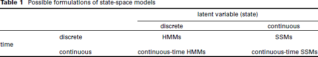
Possible formulations of state-space models
Despite these difficulties that arise when extending (discrete-time) HMMs either to have a continuous state space or to be formulated in continuous time, the corresponding extensions are nevertheless well covered in the existing literature and are fairly routinely applied. In this article, we focus on the fourth case from Table 1, that is, SSMs that are formulated in continuous time (and are not necessarily linear and Gaussian). Such models, which are not nearly as well documented in the literature as the other three classes from Table 1, are relevant in the context of irregularly sampled data in conjunction with an underlying continuous-valued state process. In particular, irregularly spaced observations are quite common in datasets on natural phenomena such as earthquakes (e.g., Beyreuther et al., (2008), in medical data (e.g., Amoros et al., (2019), or in survey data, which for example relate to psychological measurements (e.g., Oravecz et al., (2011). While continuous-time modelling can sometimes be avoided also in case of irregular sampling, for example using imputation methods as in (Kim and Stoffer (2008), continuous-time SSMs are more realistic and flexible than models that assume simplifications of either the time formulation or the nature of the latent variable. In some applications, continuous-time SSMs with a diffusion state process are considered (see, e.g., Niu et al., (2016); Lavielle (2018); Michelot et al., (2021), but except for (Albertsen et al., (2015), who use t-distributed measurement errors, both the state and the observation process are usually assumed to be linear and Gaussian to allow for the application of the Kalman filter (see, e.g., Johnson et al., 2008; Tandeo et al., 2011; Dennis and Ponciano, 2014; Koopman et al., 2018; Jonsen et al., 2020). In particular, a more general modelling framework for formulating and estimating SSMs in continuous time is still lacking. As most of the continuous-time SSMs mentioned above focus on a specific type of application, no off-the-shelf tools are readily available for general, that is, possibly non-linear and non-Gaussian modelling of irregularly spaced sequential data driven by a latent state process.
In our contribution, we present a flexible framework for continuous-time SSMs, allowing both the observation process as well as the state process to be non-linear and non-Gaussian. Our approach thus enables a variety of possible model specifications, requiring only that the transition density of the state process has an explicit analytical form (though even this can in fact be relaxed—see Section 2). The latter condition is satisfied by all linear processes, including the Ornstein-Uhlenbeck (OU) process, as well as the non-linear geometric Brownian motion and the Cox-Ingersoll-Ross process. As the model's likelihood involves intractable integration over all possible realizations of the continuous-valued state process at each observation time, we follow ideas from (Kitagawa (1987), (Bartolucci and De Luca (2003), and (Langrock (2011) and approximate the integral by finely discretizing the state space. This approximation can be regarded as a reframing of the model as a continuous-time HMM with a large but finite number of states, enabling us to apply the corresponding efficient algorithms. This state-space discretization trick to facilitate inference has in fact been used before to fit continuous-time SSMs, specifically for filtering fish movement tracks from noisy position measurements (Pedersen et al., (2008); Thygesen et al., (2009); Pedersen et al., (2011a). We apply effectively the same techniques, though presenting the model framework in general terms rather than focusing on any specific application. The key strength of the approach is its great flexibility to easily consider virtually any type of non-linear and non-Gaussian SSM, whereas most continuous-time SSMs in the literature are bound to specific applications.
In Section 2, we first discuss statistical inference for continuous-time SSMs based on approximating the likelihood via state discretization. Subsequently, in Section 3, we demonstrate the feasibility of our approach and investigate the estimation accuracy in simulation experiments. An illustrating case study on delinquent behaviour of adolescents is presented in Section 4.
We consider a sequence of random variables, 
In the following, we assume that the transition density of the state process, that is, the probability density function of
One possible choice for the state process is the OU process, which is described by the stochastic differential equation (SDE)

For simplicity of notation, we let
The likelihood of an SSM as in (2.1) can be calculated by integrating over all possible values of the state process potentially underlying each observation time, resulting in an expression involving 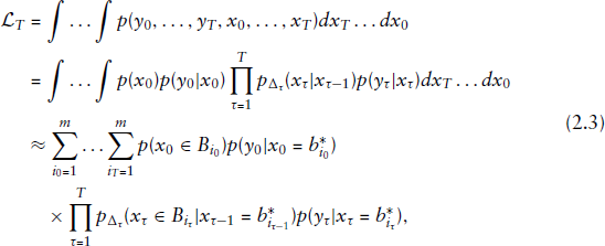
The discretization of the state space into 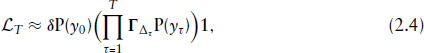
The entries in 
Irrespective of the specific assumptions made for
Simulations were conducted to explore the effect of approximating the likelihood by discretizing the continuous-valued state process, in particular with regard to the estimation accuracy. While the likelihood approximation can be rendered arbitrarily accurate by using increasingly many intervals in the discretization, it is not clear at which number of intervals
We consider three simulation settings, in which the state process is modelled using the OU process (cf. Equation (2.2)) with long-term mean 
Example path realizations of the OU processes considered. The graphs were obtained by application of the Euler-Maruyama scheme with initial value 0 and step length 0.01
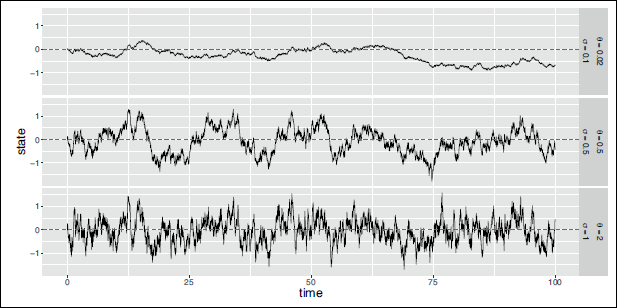
Example path realizations of the OU processes considered. The graphs were obtained by application of the Euler-Maruyama scheme with initial value 0 and step length 0.01
Estimated parameters, computation times and maximum log-likelihood (llk) values in the simulation experiments considering different numbers of intervals
used in the likelihood approximation
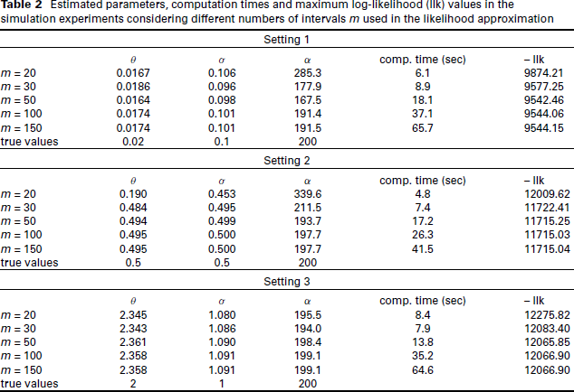
For each simulation setting and the different numbers of intervals
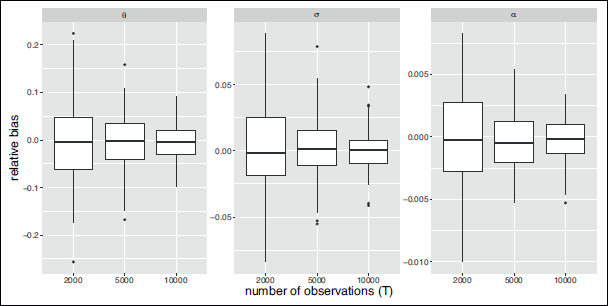
In a second simulation experiment, we ran an empirical check of the estimators’ consistency. Specifically, focusing on Setting 2 above, we simulated 200 datasets of
Boxplots of relative bias of the estimated model parameters from 200 simulation runs for
observations. True parameter values are
,
, and
Model formulation
We analyse data from the longitudinal research project Crime in the Modern City on deviant and delinquent behaviour of adolescents and young adults in Western Germany (for more details see Boers et al., (2010); Seddig and Reinecke (2017). The survey was first conducted in the year 2002 and comprised students in the 7th grade at public schools, who were mostly 12 to 13 years old. This cohort was repeatedly interviewed by means of self-administered questionnaires over a study period of 16 years. In each survey, the participants were asked about various offences like graffiti spraying, shop-lifting, drug abuse, or assault with and without a weapon, and indicated how often they had committed each offence in the twelve months prior to the survey. The data collection, however, did not follow a regular sampling scheme as the first eight waves of the panel study were administered annually, while the last four waves were conducted biannually. Further, due to wave nonresponse, meaning that some participants would not respond in one or more panel waves, the dataset contains missing values, which is quite common in longitudinal studies. As a consequence, the length of time intervals between consecutive observations is irregular and ranges from one to four years.
In this case study, we consider the total number of offences indicated in each survey, from which individual trajectories of delinquent behaviour can be constructed. We included all participants who committed at least one offence within the study period, resulting in 12 327 observations from 1 093 adolescents (467 male and 626 female). The distribution of the number of offences for different age classes and both gender is shown in Figure 3. No delinquent behaviour was most often reported (72.6% of observations), while overall the median number of offences, given that any were committed within the previous twelve months, is 3 (min: 1; max: 160).
Boxplots of the number of offences committed in the twelve months prior to the survey for different age classes and both gender. Outliers have been removed from the plot for clarity. The same figure including outliers is provided in Figure A2 in the Online Supplementary Material
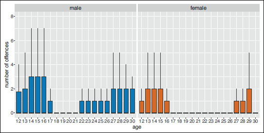
Boxplots of the number of offences committed in the twelve months prior to the survey for different age classes and both gender. Outliers have been removed from the plot for clarity. The same figure including outliers is provided in Figure A2 in the Online Supplementary Material
The main aim is to investigate the persistence of the delinquency level, which is assumed to be a latent trait underlying the observed trajectories of adolescents’ and young adults’ delinquent behaviour. Therefore, we model the number of offences using an SSM, which we formulate in continuous time to address the irregular spacing of the observations as caused by the study design and the missing data. Arguably, the data could also be regarded as a yearly time series with missing data and hence modelled using a discrete-time process—however, a continuous-time process constitutes a convenient alternative, which directly accommodates the time gaps. To allow for possible overdispersion, we assume the number of offences to follow a negative binomial distribution (conditional on the states). As the study participants’ age and gender are known to affect their delinquent behaviour (e.g., Reinecke and Weins (2013), we additionally include these covariates in the observation process. The observation process of the SSM is then specified as
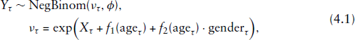
We further specify the state process to be an OU process with
To assess whether the SSM formulation is actually needed to describe the structure in the data, we additionally fit a simple generalized additive model (GAM) without an underlying state process. This benchmark model is formulated analogously as stated in Equation (4.1), omitting
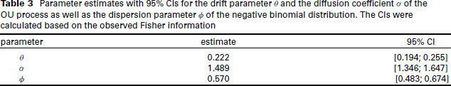
Parameter estimates with 95% CIs for the drift parameter
and the diffusion coefficient
of the OU process as well as the dispersion parameter
of the negative binomial distribution. The CIs were calculated based on the observed Fisher information
Parameter estimates with 95% CIs for the drift parameter
and the diffusion coefficient
of the OU process as well as the dispersion parameter
of the negative binomial distribution. The CIs were calculated based on the observed Fisher information
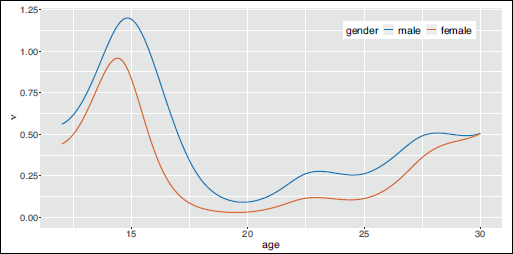
The estimated effects of age and gender on the mean parameter of the negative binomial distribution are visualised in Figure 4. While the effect of age on the expected number of offences is quite similar for both gender, female adolescents generally display a lower level of delinquent behaviour than males, which corresponds to the current state of research (e.g., Reinecke and Weins (2013). Overall, the effect of age is highly non-linear. Until the age of 14 to 15, there is an increase in delinquent behaviour, followed by a steady decline in the expected number of offences, which reflects the typical age-crime curve (e.g., Moffitt (1993). During the twenties, the expected number of offences increases again, which might here mainly be caused by data collection issues as young adults can commit additional offences that are not considered for adolescents.
Estimated effect of age on the expected number of offences for male (blue) and female (red) adolescents, respectively, given that the state equals 0
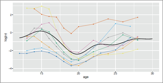
Due to transferring the SSM to an HMM framework (cf. Section 2), we can gain additional insight into the delinquency levels of individuals by using the Viterbi algorithm to infer the most probable sequence of underlying states. Based on these decoded delinquency levels as well as the individuals’ gender and age, the expected number of offences can be calculated at each observation time. Such decoded trajectories are shown for eight male adolescents in Figure 5. As a result of the underlying delinquency levels, individuals’ trajectories of the expected number of offences deviate from the overall age trend and fluctuate around the latter. Moreover, different trajectories are visible: while some adolescents have a permanently increased or reduced level of delinquency, others show early or late periods of increased delinquency levels.
Example trajectories of the logarithm of the expected number of offences for eight male individuals based on their decoded delinquency level at each observation time. The thicker, black line represents the expected trajectory for male adolescents, when their delinquency level is in equilibrium
When simulating observations based on the fitted SSM, the resulting synthetic data quite well reflect the general distribution of the number of offences observed for different age classes and both gender (cf. Figure A4 in the Online Supplementary Material). However, the simulations indicate some lack of fit with regard to the distribution of the observation process as well as to the smoothness of the underlying state process. In particular, the model can generate observations which are (much) larger than the maximum value observed in the real data due to the heavy right tail of the fitted negative binomial distribution (though this applies to only 0.23% of the simulated data). Regarding the underlying process, the simulated state trajectories tend to show stronger fluctuations in the delinquency levels than we observed in the decoded state sequences of the case study. The model fit of the continuous-time SSM might thus be improved by using a smoother process than the OU process to model the evolution of the underlying state process.
Furthermore, there are other ways in which the model formulation used in the case study could be improved and extended for a more comprehensive analysis of adolescents’ delinquent behaviour. In particular, additional variables possibly affecting the delinquency level could be considered in the model, and these could be individual-specific, time-varying, or both. Incorporating time-varying covariates into the continuous-time state process is rather challenging as it renders the likelihood calculation analytically intractable. An important exception is the case where the covariate of interest is piecewise constant over time (see, e.g., Faddy, 1976; Kay, 1986). Moreover, the current model formulation does not account for possible heterogeneity across survey participants. As indicated in Figure 5, some adolescents’ expected delinquency is consistently higher or lower than the population mean, which could be addressed for example by modelling the long-term mean
Finally, it is not a priori clear if the data are more adequately modelled using a continuous- or discrete-valued underlying state process. Comparing our SSM to 2- to 5-state HMMs reveals that based on the AIC, continuous-time HMMs with more than two states are favoured over the SSM assuming a continuous state space (cf. Table A1 in the Online Supplementary Material). However, choosing an adequate number of latent delinquency levels comes with its own challenges. In particular, for HMM-like models, the AIC generally tends to select models with a larger than plausible number of states—in our case the 5-state model was chosen, but without us testing higher-order models—hence impeding a meaningful interpretation of the states (see, e.g., Pohle et al., (2017). Overall, the case study illustrates the versatility of our modelling and the associated inferential framework, for example regarding the specification of non-Gaussian distributions in the observation process as well as nonparametric covariate effects.
In this contribution, we developed a flexible framework for formulating and estimating general continuous-time SSMs. These are latent-state models suited to sequential observations that are irregularly spaced in time, that is, data to which discrete-time models are not (directly) applicable. In some applications, for example in biology (e.g., Runde et al., (2020), psychology (e.g., de Haan-Rietdijk et al., (2017), or finance (e.g., Kim and Stoffer (2008), irregularly spaced observations are simply treated as if they do follow a regular sampling scheme, or are forced into a sequence with regular (i.e., equidistant) time intervals based on data aggregation or imputation. These aggregated or imputed data are then analysed using discrete-time models, which are less technically challenging than their continuous-time counterparts. However, temporal aggregation of continuous-time processes discards information on the exact observation times and introduces subjectivity concerning the choice of the discrete-time modelling resolution, while imputation methods for generating regular time intervals introduce additional uncertainty, which is why both approaches possibly produce biased estimates (see, e.g., Yip and Wang (2002); Delsing et al., (2005); Barbour et al., (2013); Kleinke et al., (2021). Therefore, continuous-time models are generally preferable when data are collected at irregular points in time. These models are not only conceptually appealing as their interpretation does not depend on the time resolution of the data at hand, but also avoid the pitfalls mentioned above. These benefits come at the cost of increased mathematical and computational complexity, especially for the case of SSMs with non-linear and non-Gaussian processes.
While we are not the first to consider continuous-time SSMs, existing models often focus on a particular data application and hence are very case-specific (e.g., Dennis and Ponciano (2014); Albertsen et al., (2015); Niu et al., (2016). In particular, existing approaches usually make restrictive model assumptions to simplify parameter estimation, for example requiring the SSM to be linear and Gaussian to enable the application of the Kalman filter (e.g., Johnson et al., (2008); Tandeo et al., (2011); Koopman et al., (2018); Lavielle (2018); Jonsen et al., (2020). In contrast, the maximum (approximate) likelihood approach we propose here is not tied to specific distributional or linearity assumptions, thus allowing for both non-linear and non-Gaussian specifications of the state and observation process. Our method, however, is by no means the only method to fit continuous-time SSMs: Apart from the Kalman filter, which can be used for linear and Gaussian SSMs, MCMC methods (Niu et al., (2016) and Laplace approximation techniques (Albertsen et al., (2015); Michelot et al., (2021) as implemented in the R-package Template Model Builder (Kristensen et al., (2016) have been developed for statistical inference in continuous-time SSMs. While the modelling approach presented here is not assumed to be superior to such alternative estimation techniques, it offers the convenience of the continuous-time HMM framework and its corresponding efficient algorithms. The latter proves beneficial not only with respect to model fitting but also for decoding the most probable underlying state trajectories. Moreover, only minor changes in the corresponding code for the likelihood calculation are required to consider different distributions or non-linear relationships in either the observation or state process, provided that the transition density is known in explicit form. A major caveat of the approach, however, is that it suffers from a curse of dimensionality when considering multivariate state processes (e.g., Langrock (2011). In conclusion, our approach constitutes an accessible and very flexible framework for modelling irregularly spaced sequential data driven by a one-dimensional underlying state process.
Supplementary material
In the Online Supplementary Material, we provide the R code for the simulation experiments conducted in Section 3 and the R code used for the case study. The data for the case study cannot be shared due to privacy, but is available on request from the authors. Therefore, artificially simulated data based on the case study results and structured exactly as the real data is available for illustration. The supplementary material can be found at:
Footnotes
Declaration of conflicting interests
The authors declared no potential conflicts of interest with respect to the research, authorship and/or publication of this article.
Funding
The authors disclosed the receipt of the following financial support for the research, authorship and/or publication of this article: This research was funded by the German Research Foundation (DFG) as part of the SFB TRR 212 (NC3)-Projektnummer 316099922.
Acknowledgments
We would like to thank Christiane Fuchs for her valuable input on SDEs. We are also grateful to two anonymous reviewers for their insightful and very useful feedback that helped us to improve this article.