Multivariate functional additive mixed models

Abstract

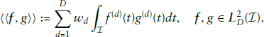
Multivariate functional data can be intrinsically multivariate like movement trajectories in 2D or complementary such as precipitation, temperature and wind speeds over time at a given weather station. We propose a multivariate functional additive mixed model (multiFAMM) and show its application to both data situations using examples from sports science (movement trajectories of snooker players) and phonetic science (acoustic signals and articulation of consonants). The approach includes linear and nonlinear covariate effects and models the dependency structure between the dimensions of the responses using multivariate functional principal component analysis. Multivariate functional random intercepts capture both the auto-correlation within a given function and cross-correlations between the multivariate functional dimensions. They also allow us to model between-function correlations as induced by, for example, repeated measurements or crossed study designs. Modelling the dependency structure between the dimensions can generate additional insight into the properties of the multivariate functional process, improves the estimation of random effects, and yields corrected confidence bands for covariate effects. Extensive simulation studies indicate that a multivariate modelling approach is more parsimonious than fitting independent univariate models to the data while maintaining or improving model fit.

1 Introduction

With the technological advances seen in recent years, functional datasets are increasingly multivariate. They can be multivariate with respect to the domain of a function, its codomain, or both. Here, we focus on multivariate functions with a one-dimensional domain $\mathbf{f}=(f^{(1)},...,f^{(D)}):\mathcal{I}\subset \mathbb{ℝ}\to {\mathbb{ℝ}}^D$ with square-integrable components $f^{(d)}\in L^2(\mathcal{I}),d=1,...,D$ . For this type of data, we can distinguish two subclasses: One has interpretable separate dimensions and can be seen as several complementary modes of a common phenomenon (‘multimodal’ data, cf. Uludağ and Roebroeck, 2014) as in the analysis of acoustic signals and articulation processes in speech production in one of our data examples. The codomain then simply is the Cartesian product $\mathcal{S}={\mathcal{S}}^{(1)}\times ...\times {\mathcal{S}}^{(D)}$ of interpretable univariate codomains ${\mathcal{S}}^{(d)}\subset \mathbb{ℝ}$ . The other subclass is more ‘intrinsically’ multivariate insofar as univariate analyses would not yield meaningful results. Consider for example two-dimensional movement trajectories as in one of our motivating applications, where the function measures Cartesian coordinates over time: for fixed trajectories, rotation or translation of the essentially arbitrary coordinate system would change the results of univariate analyses. For intrinsically multivariate functional data a multivariate approach is the natural and preferred mode of analysis, yielding interpretable results on the observation level. Even for multimodal functional data, a joint analysis may generate additional insight by incorporating the covariance structure between the dimensions. This motivates the development of statistical methods for multivariate functional data. We here propose multivariate functional additive mixed models to model potentially sparsely observed functions with flexible covariate effects and crossed or nested study designs.

Multivariate functional data have been the interest in different statistical fields such as clustering (Jacques and Preda, 2014; Park and Ahn, 2017), functional principal component analysis (FPCAs) (Chiou et al., 2014; Happ and Greven, 2018; Backenroth et al., 2018; Li et al., 2020), and registration (Carroll et al., 2021; Steyer et al., 2021). There is also ample literature on multivariate functional data regression such as graphical models (Zhu et al., 2016), reduced rank regression (Liu et al., 2020), or varying coefficient models (Zhu et al., 2012; Li et al., 2017). Yet, so far, there are only few approaches that can handle multilevel regression when the functional response is multivariate. In particular, Goldsmith and Kitago (2016) propose a hierarchical Bayesian multivariate functional regression model that can include subject level and residual random effect functions to account for correlation between and within functions. They work with bivariate functional data observed on a regular and dense grid and assume a priori independence between the different dimensions of the subject-specific random effects. Thus, they model the correlation between the dimensions only in the residual function. As our approach explicitly models the dependencies between dimensions for multiple functional random effects and also handles data observed on sparse and irregular grids on more than two dimensions, the model proposed by Goldsmith and Kitago (2016) can be seen as a special case of our more general model class.

Alternatively, Zhu et al. (2017) use a two-stage transformation with basis functions for the multivariate functional mixed model. This allows the estimation of scalar regression models for the resulting basis coefficients that are argued to be approximately independent. The proposed model is part of the so-called functional mixed model (FMM) framework (Morris, 2017). While FMMs use basis transformations of functional responses (observed on equal grids) at the start of the analysis, we propose a multivariate model in the functional additive mixed model (FAMM) framework, which uses basis representations of all (effect) functions in the model (Scheipl et al., 2015). The differences between these two functional regression frameworks have been extensively discussed before (Greven and Scheipl, 2017; Morris, 2017).

The main advantages of our multivariate regression model, also compared to Goldsmith and Kitago (2016) and Zhu et al. (2017), are that it is readily available for sparse and irregular functional data and that it allows to include multiple nested or crossed random processes, both of which are required in our data examples. Another important contribution is that our approach directly models the multivariate covariance structure of all random effects included in the model using multivariate functional principal components (FPCs) and thus implicitly models the covariances between the dimensions. This makes the model representation more parsimonious, avoids assumptions difficult to verify, and allows further interpretation of the random effect processes, such as their relative importance and their dominating modes. As part of the FAMMframework, our model provides a vast toolkit of modelling options for covariate and random effects, of estimation and inference (Wood, 2017). The proposed multivariate functional additive mixed model (multiFAMM) extends the FAMM framework combining ideas from multilevel modelling (Cederbaum et al., 2016) and multivariate functional data (Happ and Greven, 2018) to account for sparse and irregular functional data and different study designs.

We illustrate the multiFAMM on two motivating examples. The first (intrinsically multivariate) data stem from a study on the effect of a training programme for snooker players with a nested study design (shots within sessions within players) (Enghofer, 2014). The movement trajectories of a player's elbow, hand, and shoulder during a snooker shot are recorded on camera, yielding six-dimensional multivariate functional data (see Figure 1). In the second data example, we analyse multimodal data from a speech production study with a crossed study design (speakers crossed with words) (Pouplier and Hoole, 2016) on so-called ‘assimilation’ of consonants. The two measured modes (acoustic and articulatory, see Figure 3) are expected to be closely related but joint analyses have not yet incorporated the functional nature of the data.

These two examples motivate the development of a regression model for sparse and irregularly sampled multivariate functional data that can incorporate crossed or nested functional random effects as required by the study design in addition to flexible covariate effects. The proposed approach is implemented in R (R Core Team, 2020) in package multifamm (Volkmann, 2021). The article is structured as follows: Section 2 specifies the multiFAMM and Section 3 its estimation process. Section 4 presents the application of the multiFAMM to the data examples and Section 5 shows the estimation performance of our proposed approach in simulations. Section 6 closes with a discussion and outlook.

2 Multivariate functional additive mixed model

2.1 General model

Let ${\mathbf{y}}_i^{*}(t)=(y_i^{*(1)}(t),...,y_i^{*(D)}(t){)}^{\top }$ be the multivariate functional response of unit $i=1,...,N$ over $t\in \mathcal{I}$ , consisting of dimensions $d=1,...,D$ . Without loss of generality, we assume a common one-dimensional interval domain $\mathcal{I}=[0,1]$ for all dimensions, and square-integrable $y_i^{*(d)}\in L^2(\mathcal{I})$ . Define $L_D^2(\mathcal{I}):=L^2(\mathcal{I})\times ...\times L^2(\mathcal{I})$ so that ${\mathbf{y}}_i^{*}\in L_D^2(\mathcal{I})$ . The underlying smooth function ${\mathbf{y}}_i^{*}$ , however, is only evaluated at (potentially sparse or dimension specific) points ${\mathbf{y}}_{\mathit{it}}^{*}=(y_{\mathit{it}}^{*(1)},...,y_{\mathit{it}}^{*(D)}{)}^{\top }$ and the evaluation is subject to white noise, that is, ${\mathbf{y}}_{\mathit{it}}={\mathbf{y}}_{\mathit{it}}^{*}+{\mathbf{\epsilon }}_{\mathit{it}}$ . The residual term ${\mathbf{\epsilon }}_{\mathit{it}}$ reflects additional uncorrelated white noise measurement error, following a $D$ -dimensional multivariate normal distribution ${\mathcal{N}}_D$ with zero-mean and diagonal covariance matrix $\tilde{\mathbf{\Sigma }}=\mathrm{diag}({\sigma }_1^2,...,{\sigma }_D^2)$ with dimension-specific variances ${\sigma }_d^2$ . We construct a multivariate functional mixed model as

$$\begin{array}{c}{y}_{it}=y_i^{*}(t)+{ϵ}_{it}=\mu \left(x_i,t\right)+U(t)z_i+{ϵ}_{it}\\ =\mu \left(x_i,t\right)+{\displaystyle \sum _{j=1}^q{U}_j}(t)z_{ij}+E_i(t)+{ϵ}_{it},t\in \mathcal{I},\end{array}$$

(2.1)

where

$$\begin{array}{c}{U}_j(t)=\left(U_{i1}(t),\dots ,U_{iV}(t)\right);j=1,\dots ,q\\ U_{jv}(t)\stackrel{\text{ ind}.\text{c}. }{~}MGP\left(0,K_{U_i}\right);v=1,\dots ,V_{U_i};\forall j=1,\dots ,q\text{,}\\ E_i(t)\stackrel{\text{ ind}.\text{c}. }{~}MGP\left(0,K_E\right);i=1,\dots ,N\text{, and}\\ {ϵ}_{it}\stackrel{\text{ i}.\text{i}.\text{d}. }{~}{\mathcal{N}}_D\left(0,\tilde{\Sigma }=\mathrm{diag}\left({\sigma }_1^2,\dots ,{\sigma }_D^2\right)\right);i=1,\dots ,N;t\in \mathcal{I}.\end{array}$$

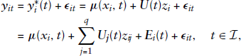
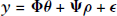
We assume an additive predictor $\mathbf{\mu }({\mathbf{x}}_i,·)={\sum }_{l=1}^p{\mathbf{f}}_l({\mathbf{x}}_i,·)$ of fixed effects, which consists of partial predictors ${\mathbf{f}}_l({\mathbf{x}}_i,·)=(f_l^{(1)}({\mathbf{x}}_i,·),...,f_l^{(D)}({\mathbf{x}}_i,·){)}^{\top }\in L_D^2(\mathcal{I}), l=1,...,p$ , that are multivariate functions depending on a subset of the vector of scalar covariates ${\mathbf{x}}_i$ . This allows to include linear or smooth covariate effects as well as interaction effects between multiple covariates as in the univariate FAMM (Scheipl et al., 2015). Partial predictors may also depend on dimension-specific subsets of covariates.

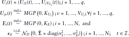
For random effects $\mathbf{U}$ , we focus on model scenarios with $q$ independent multivariate functional random intercepts for crossed and/or nested designs. For group level $v=1,\dots ,V_{U_j}$ within grouping layer $j=1,\dots ,q$ , these take the value ${\mathbf{U}}_{\mathit{jv}}\in L_D^2(\mathcal{I})$ . For each layer, the ${\mathbf{U}}_{j1},...,{\mathbf{U}}_{{\mathit{jV}}_{U_j}}$ present independent copies of a multivariate smooth zero-mean Gaussian random process. Analogously to scalar linear mixed models, the ${\mathbf{U}}_{\mathit{jv}}$ model correlations between different response functions ${\mathbf{y}}_i^{*}$ within the same group as well as variation across groups. By arranging them in a $(D\times V_{U_j})$ matrix ${\mathbf{U}}_j(t)$ per $t$ , the $j$ th random intercept can be expressed in the common mixed model notation in (2.1) using appropriate group indicators ${\mathbf{z}}_{\mathit{ij}}=(z_{\mathit{ij}1},\dots ,z_{{\mathit{ijV}}_{U_j}}{)}^{\top }$ for the respective design.

Although technically a curve-specific functional random intercept, we distinguish the smooth residuals ${\mathbf{E}}_i\in L_D^2(\mathcal{I})$ in the notation, as they model correlation within rather than between response functions. We write ${\mathbf{E}}_v\in L_D^2(\mathcal{I}),v=1,...,V_E$ with $V_E=N$ . The ${\mathbf{E}}_i$ capture smooth deviations from the group-specific mean $\mathbf{\mu }({\mathbf{x}}_i,·)+{\sum }_{j=1}^q{\mathbf{U}}_j(·){\mathbf{z}}_{\mathit{ij}}$ .

For a more compact representation, we can arrange all ${\mathbf{U}}_j(t)$ and ${\mathbf{E}}_i(t)$ together in a $(D\times ({\sum }_{j=1}^q{V}_{U_j}+N))$ matrix $\mathbf{U}(t)$ per $t$ , and the group indicators for all layers in a corresponding vector ${\mathbf{z}}_i=({\mathbf{z}}_{i1}^{\top },\dots ,{\mathbf{z}}_{\mathit{iq}}^{\top },{\mathbf{e}}_i^{\top }{)}^{\top }$ with ${\mathbf{e}}_i$ the $i$ -th unit vector. The resulting model term $\mathbf{U}(t){\mathbf{z}}_i$ then comprises all smooth random functions, accounting for all correlation between/within response functions ${\mathbf{y}}_i^{*}$ given the covariates ${\mathbf{x}}_i$ as required by the respective experimental design.

${\mathbf{E}}_i$ and ${\mathbf{U}}_{\mathit{jv}}$ are independent copies (ind. c.) of random processes having multivariate $D\times D$ covariance kernels $K_E,K_{U_j}$ , with univariate covariance surfaces $K_E^{(d,e)}(t,t^{\prime })=\mathit{Cov}\left[E_i^{(d)}(t),E_i^{(e)}(t^{\prime })\right]$ and $K_{U_j}^{(d,e)}(t,t^{\prime })=\mathit{Cov}\left[U_{\mathit{jv}}^{(d)}(t),U_{\mathit{jv}}^{(e)}(t^{\prime })\right]$ reflecting the covariance between the process dimensions $d$ and $e$ at $t$ and $t^{\prime }$ . We call these auto-covariances for $d=e$ and cross-covariance otherwise. The multivariate Gaussian processes are uniquely defined by their multivariate mean function, here the null function $0$ , and the multivariate covariance kernels $K_g$ and we write $\mathit{MGP}\left(0,K_g\right),g\in \{U_1,\dots ,U_q,E\}$ . Note that vectorizing the matrix $\mathbf{U}(t)$ allows to formulate the joint distribution assumption $\mathrm{vec}(\mathbf{U}(t))\sim \mathit{MGP}\left(0,K_U\right)$ with $K_U(t,t^{\prime })$ having a block-diagonal structure repeating each $K_{U_j}(t,t^{\prime })$ for $V_{U_j}$ times and $K_E(t,t^{\prime })$ for $N$ times.

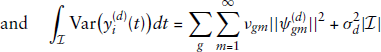
We assume that the different sources of variation ${\mathbf{U}}_j(t),j=1,...,q,{\mathbf{E}}_i(t)$ , and ${\mathbf{\epsilon }}_{\mathit{it}}$ are mutually uncorrelated random processes to assure model identification. Assuming smoothness of the covariance kernel $K_E$ further guarantees that the residual process ${\mathbf{E}}_i(t)$ can be separated from the white noise ${\mathbf{\epsilon }}_{\mathit{it}}$ , removing the error variance from the diagonal of the smooth covariance kernel (e.g., Yao et al., 2005).

2.2 FPC representation of the random effects

Model (2.1) specifies a univariate functional linear mixed model (FLMM) as given in Cederbaum et al. (2016) for each dimension $d$ . The main difference lies in the multivariate random processes that introduce dependencies between the dimensions. In order to avoid restrictive assumptions about the structure of these multivariate covariance operators, which would typically be very difficult to elicit a priori or verify ex post, we estimate them directly from the data. The main difficulty then becomes computationally efficient estimation, which is already costly in the univariate case. Especially for higher dimensional multivariate functional data, accounting for the cross-covariances can become a complex task, which we tackle with multivariate functional principal component analysis (MFPCA).

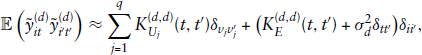
Given the covariance operators (see Section 3), we represent the multivariate random effects in Model (2.1) using truncated multivariate Karhunen-Loève (KL) expansions

$$\begin{array}{l}{U}_{jv}(t)\approx {\displaystyle \sum _{m=1}^{M_{U_j}}{\rho }_{U_{j}vm}}{\psi }_{U_{j}m}(t),j=1,\dots ,q;v=1,\dots ,V_{U_i},\\ E_v(t)\approx {\displaystyle \sum _{m=1}^{M_E}{\rho }_{Evm}}{\psi }_{Em}(t),v=1,\dots ,N,\end{array}$$

(2.2)

where the orthonormal multivariate eigenfunctions ${\mathbf{\psi }}_{\mathit{gm}}=({\psi }_{\mathit{gm}}^{(1)},...,{\psi }_{\mathit{gm}}^{(D)}{)}^{\top }\in L_D^2(\mathcal{I})$ , $m=1,...,M_g$ , $g\in \{U_1,...,U_q,E\}$ of the corresponding covariance operators with truncation order $M_g$ are used as basis functions and the random scores ${\rho }_{\mathit{gvm}}\sim N(0,{\nu }_{\mathit{gm}})$ are independent and identically distributed (i.i.d.) with ordered eigenvalues ${\nu }_{\mathit{gm}}$ of the corresponding covariance operator. Note that the assumption of Gaussianity for the random processes can be relaxed. For non-Gaussian random processes, the KL expansion still gives uncorrelated (but non-normal) scores and estimation based on a penalized least squares (PLS) criterion (see Section 3.2) remains reasonable.

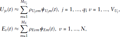
Using KL expansions gives a parsimonious representation of the multivariate random processes that is an optimal approximation with respect to the integrated squared error (cf. Ramsay and Silverman, 2005), as well as interpretable basis functions capturing the most prominent modes of variation of the respective process. The distinct feature of this approach is that the multivariate FPCs directly account for the dependency structure of each random process across the dimensions. If, by contrast, for example, splines were used in the basis representation of the random effects, it would be necessary to explicitly model the cross-covariances of each random process in the model (cf. Li et al., 2020). Multivariate eigenfunctions, however, are designed to incorporate the dependency structure between dimensions and allow the assumption of independent (univariate) basis coefficients ${\rho }_{\mathit{gvm}}$ via the KL theorem (see, e.g., Happ and Greven, 2018). This leads to a parsimonious multivariate basis for the random effects, where a typically small vector of scalar scores ${\rho }_{\mathit{gvm}}$ common to all dimensions represents nearly the entire information about these $D$ -dimensional processes.

3 Estimation

We use a two-step approach to estimate the multiFAMM and the respective multivariate covariance operators. In a first step (Section 3.1), the D-dimensional eigenfunctions ${\mathbf{\psi }}_{\mathit{gm}}(t)$ with their corresponding eigenvalues ${\nu }_{\mathit{gm}}$ are estimated from their univariate counterparts following Cederbaum et al. (2018) and Happ and Greven (2018). These estimates are then plugged into (2.2) and we represent the multiFAMM as part of the general FAMM framework (Section 3.2) by suitable re-arrangement. We can view the estimated ${\mathbf{\psi }}_{\mathit{gm}}(t)$ simply as an empirically derived basis that parsimoniously represents the patterns in the observed data. While their estimation adds uncertainty, we are not interested in inferential statements for the variance modes and our simulations (see Section 5) suggest that the estimated eigenfunctions are reasonable approximations that work well as a basis.

3.1 Step 1: Estimation of the eigenfunction basis

3.1.1 Step 1 (i): Univariate mean estimation

In a first step, we obtain preliminary estimates of the dimension-specific means ${\mu }^{(d)}({\mathbf{x}}_i,t)={\sum }_{l=1}^p{f}_l^{(d)}({\mathbf{x}}_{\mathit{il}},t)$ using univariate FAMMs. We model

$$\begin{array}{cc}{y}_{\mathit{it}}^{(d)}\hfill & ={\mu }^{(d)}({\mathbf{x}}_i,t)+{\epsilon }_{\mathit{it}}^{(d)}; d=1,\dots ,D\hfill \end{array}$$

(3.1)

independently for all $d$ with i.i.d. Gaussian random variables ${\epsilon }_{\mathit{it}}^{(d)}$ . The estimation of ${\mu }^{(d)}({\mathbf{x}}_i,t)$ proceeds analogously to the estimation of the multiFAMM described in Section 3.2. It is based on the evaluation points of the $y_i^{*(d)}(t)$ , whose locations on the interval $\mathcal{I}$ can vary across dimensions. Model (3.1) thus accommodates sparse and irregular multivariate functional data and implies a working independence assumption across scalar observations within and across functions.

3.1.2 Step 1 (ii): Univariate covariance estimation

This preliminary mean function is used to centre the data ${\tilde{y}}_{\mathit{it}}^{(d)}=y_{\mathit{it}}^{(d)}-{\widehat{\mu }}^{(d)}({\mathbf{x}}_i,t)$ in order to obtain noisy evaluations of the detrended functions ${\tilde{y}}_i^{*(d)}(t)=y_i^{*(d)}(t)-{\mu }^{(d)}({\mathbf{x}}_i,t)$ for covariance estimation. Cederbaum et al. (2016) already find that for this purpose, the working independence assumption within functions across evaluation points in (3.1) gives reasonable results. The expectation of the crossproducts of the centred functions then coincides with the auto-covariance, that is, $\mathbb{}\left({\tilde{y}}_{\mathit{it}}^{(d)}{\tilde{y}}_{i^{\prime }{t}^{\prime }}^{(d)}\right)\approx \mathit{Cov}\left[y_{\mathit{it}}^{(d)},y_{i^{\prime }{t}^{\prime }}^{(d)}\right]$ . For the independent random components specified in Model (2.1), this overall covariance decomposes additively into contributions from each random process as

$$\begin{array}{cc}\mathbb{}\left({\tilde{y}}_{\mathit{it}}^{(d)}{\tilde{y}}_{i^{\prime }{t}^{\prime }}^{(d)}\right)\approx \sum _{j=1}^q{K}_{U_j}^{(d,d)}(t,t^{\prime }){\delta }_{v_j{v}_j^{\prime }}+(K_E^{(d,d)}(t,t^{\prime })+{\sigma }_d^2{\delta }_{{\mathit{tt}}^{\prime }}){\delta }_{{\mathit{ii}}^{\prime }},\hfill & \hfill \end{array}$$

(3.2)

using indicators ${\delta }_{{\mathit{xx}}^{\prime }}$ that equal one for $x=x^{\prime }$ and zero otherwise. The indicator ${\delta }_{v_j{v}_j^{\prime }}$ thus identifies if the curves in the crossproduct belong to the same group $v_j$ of the $j$ th layer. Using $t$ , $t^{\prime }$ , and the indicators ${\delta }_{v_j{v}_j^{\prime }},{\delta }_{{\mathit{tt}}^{\prime }},{\delta }_{{\mathit{ii}}^{\prime }}$ as covariates and the crossproducts of the centred data as responses, we can estimate the auto-covariances $K_{U_1}^{(d,d)},...,K_{U_q}^{(d,d)},$ and $K_E^{(d,d)}$ of the random processes using symmetric additive covariance smoothing (Cederbaum et al., 2018). This extends the univariate approach proposed by Cederbaum et al. (2016). In particular, we also allow a nested random effects structure as required for the snooker training application in Section 4.1 by specifying the indicator of the nested effect as the product of subject-and-session indicators. Note that estimating (3.2) also yields estimates of the dimension-specific error variances ${\sigma }_d^2$ as a byproduct.

3.1.3 Step 1 (iii): Univariate eigenfunction estimation

Based on the covariance kernel estimates, we apply separate univariate FPCAs for each random process by conducting an eigendecomposition of the respective linear integral operator. Practically, each estimated process- and dimension-specific auto-covariance is re-evaluated on a dense grid so that a univariate functional principal component analysis (FPCA) can be conducted. Alternatively, Reiss and Xu (2020) provide an explicit spline representation of the estimated eigenfunctions. Eigenfunctions with non-positive eigenvalues are removed to ensure positive definiteness, and further regularization by truncation based on the proportion of variance explained is possible (see, e.g., Di et al., 2009; Peng and Paul, 2009; Cederbaum et al., 2016). However, we suggest to keep all univariate FPCs with positive eigenvalues for the computation of the MFPCA in order to preserve all important modes of variation and cross-correlation in the data.

3.1.4 Step 1 (iv): Multivariate eigenfunction estimation

The estimated univariate eigenfunctions and scores are then used to conduct an MFPCA for each of the $g$ multivariate random processes separately. The MFPCA exploits correlations between univariate FPC scores across dimensions to reduce the number of basis functions needed to sufficiently represent the random processes. We base the MFPCA on the following definition of a (weighted) scalar product

$$\begin{array}{cc}⟨⟨\mathbf{f},\mathbf{g}⟩⟩:=\sum _{d=1}^D{w}_d{\int }_{\mathcal{I}}{f}^{(d)}(t)g^{(d)}(t)\mathit{dt},\mathbf{f},\mathbf{g}\in L_D^2(\mathcal{I}),\hfill & \hfill \end{array}$$

(3.3)

for the response space with positive weights $w_d,d=1,...,D$ and the induced norm denoted by $|||·|||$ . The corresponding covariance operators ${\Gamma }_g:L_D^2(\mathcal{I})\to L_D^2(\mathcal{I})$ of the multivariate random processes ${\mathbf{U}}_{\mathit{jv}}$ and ${\mathbf{E}}_v$ are then given by $({\Gamma }_g\mathbf{f})(t)=⟨⟨\mathbf{f},K_g(t,·)⟩⟩$ , $g\in \{U_1,...,U_q,E\}$ . The standard choice of weights in our applications is $w_1=...=w_D=1$ (unweighted scalar product) but other choices are possible. Consider for example a scenario where dimensions are observed with different amounts of measurement error. If variation in dimensions with a large proportion of measurement error is to be downweighted, we propose to use $w_d=\frac{1}{{\widehat{\sigma }}_d^2}$ with the dimension-specific measurement error variance estimates ${\widehat{\sigma }}_d^2$ obtained from (3.2).

Happ and Greven (2018) show that estimates of the multivariate eigenvalues ${\nu }_{\mathit{gm}}$ of ${\Gamma }_g$ can be obtained from an eigenanalysis of a covariance matrix of the univariate random scores. The corresponding multivariate eigenfunctions ${\mathbf{\psi }}_{\mathit{gm}}$ can be obtained as linear combinations of the univariate eigenfunctions with the weights given by the resulting eigenvectors. The estimates ${\widehat{\mathbf{\psi }}}_{\mathit{gm}}$ are then substituted for the basis functions of the truncated multivariate KL expansions of the random effects ${\mathbf{U}}_{\mathit{jv}}$ and ${\mathbf{E}}_v$ in (2.2). Note that for each random process $g$ , the maximum number of FPCs is given by the total number of univariate eigenfunctions included in the estimation process of the MFPCA of $g$ . To achieve further regularization and analogously to Cederbaum et al. (2016), we propose to choose truncation orders $M_g$ for each KL expansion of the multivariate random processes using a prespecified proportion of explained variation.

3.1.5 Step 1 (v): Multivariate truncation order

We offer two different approaches for the choice of truncation orders $M_g$ based on different variance decompositions (derivation in Supplementary Material A):

$$\mathbb{E}\left(\Vert {\left|y_i-\mu \left(x_i\right)\Vert \right|}^2)={\displaystyle \sum _{d=1}^D{w}_d}{\displaystyle {\int }_{\mathcal{I}}\mathrm{Var}}\left(y_i^{(d)}(t)\right)dt={\displaystyle \sum _g{\displaystyle \sum _{m=1}^{\infty }{v}_{gm}}}+{\displaystyle \sum _{d=1}^D{w}_d}{\sigma }_d^2|\mathcal{I}|\right.,$$

(3.4)

$$\text{and}{\displaystyle {\int }_{\mathcal{I}}\mathrm{Var}}\left(y_i^{(d)}(t)\right)dt={\displaystyle \sum _g{\displaystyle \sum _{m=1}^{\infty }{v}_{gm}}}{‖{\psi }_{gm}^{(d)}‖}^2+{\sigma }_d^2\left|\mathcal{I}\right|$$

(3.5)

with $|\mathcal{I}|$ the length of the interval $\mathcal{I}$ (here equal to one) and $||·||$ the $L^2$ norm. Multivariate variance decomposition (304) uses the (weighted) sum of total variation in the data across dimensions. We select the FPCs with highest associated eigenvalues ${\nu }_{\mathit{gm}}$ over all random processes $g$ until their sum reaches a prespecified proportion (e.g., 0.95) of the total variation, thus approximating the infinite sums in (3.5) with $M_g$ summands. For the approach based on the univariate variance (3.5), we require $M_g$ to be the smallest truncation order for which at least a prespecified proportion of variance is explained on every dimension $d$ . This second choice of $M_g$ might be preferable in situations where the variation is considerably different (in amount or structure) across dimensions, whereas the first approach gives a more parsimonious representation of the random effects. Note that both approaches can lead to a simplification of the multiFAMM if $M_g=0$ is chosen for some $g$ . The simulation results of Section 5 suggest that increasing the number of FPCs improves model accuracy which is why sensitivity analyses with regard to the truncation order are recommended.

3.2 Step 2: Estimation of the multiFAMM

In the following, we discuss estimating the multiFAMM given the estimated multivariate FPCs. We base the proposed model on the general FAMM framework of Scheipl et al. (2015), which models functional responses using basis representations. To make the extension of the FAMM framework to multivariate functional data more apparent, the multivariate response vectors and the respective model matrices are stacked over dimensions, so that every block has the structure of a univariate FAMM over all observations $i$ . This gives concatenated basis functions with discontinuities between the dimensions. The fixed effects are modelled analogously to the univariate case by interacting all covariate effects with a dimension indicator. The random effects are based on the parsimonious, concatenated multivariate FPC basis.

3.2.1 Matrix representation

For notational simplicity we assume that the functions are evaluated on a fixed grid of time points $\mathbf{t}=({\mathbf{t}}^{(1)\top },...,{\mathbf{t}}^{(D)\top }{)}^{\top }$ with ${\mathbf{t}}^{(d)\top }=({\mathbf{t}}_1^{(d)},...,{\mathbf{t}}_N^{(d)\top })$ and identical ${\mathbf{t}}_i^{(d)}\equiv (t_1,...,t_T{)}^{\top }$ over all $N$ individuals and $D$ dimensions. However, our framework allows for sparse functional data using different grids per dimension and per observed function as in the two applications (Section 4). Correspondingly, $\mathbf{y}=({\mathbf{y}}^{(1)\top },...,{\mathbf{y}}^{(D)\top }{)}^{\top }$ is the $\mathit{DNT}$ -vector of stacked evaluation points with ${\mathbf{y}}^{(d)}=({\mathbf{y}}_1^{(d)\top },...,{\mathbf{y}}_N^{(d)\top }{)}^{\top }$ and ${\mathbf{y}}_i^{(d)}=(y_{i1}^{(d)},...,y_{\mathit{iT}}^{(d)}{)}^{\top }$ . Model (2.1) on this grid can be written as

$$\begin{array}{cc}\mathbf{y}=\Phi \theta +\Psi \rho +\mathbf{\epsilon }\hfill & \hfill \end{array}$$

(3.6)

with $\mathbf{\Phi },\mathbf{\Psi }$ the model matrices for the fixed and random effects, respectively, $\mathbf{\theta },\mathbf{\rho }$ the vectors of coefficients and random effect scores to be estimated, and $\mathbf{\epsilon }=({\mathbf{\epsilon }}^{(1)\top },...,{\mathbf{\epsilon }}^{(D)\top }{)}^{\top }$ , ${\mathbf{\epsilon }}^{(d)}=({\epsilon }_{11}^{(d)},...,{\epsilon }_{1T}^{(d)},...,{\epsilon }_{\mathit{NT}}^{(d)}{)}^{\top }$ the vector of residuals. We have $\mathbf{\epsilon }\sim N(0,\mathbf{\Sigma })$ with $\mathbf{\Sigma }=\mathrm{diag}({\sigma }_1^2,...,{\sigma }_D^2)\otimes {\mathbf{I}}_{\mathit{NT}}$ , the Kronecker product denoted by $\otimes$ , and the $(\mathit{NT}\times \mathit{NT})$ identity matrix ${\mathbf{I}}_{\mathit{NT}}$ .

We estimate $\mathbf{\theta }$ and $\mathbf{\rho }$ by minimizing the PLS criterion

$$\begin{array}{cc}(\mathbf{y}-\Phi \theta -\Psi \rho ){\mathbf{\Sigma }}^{-1}(\mathbf{y}-\Phi \theta -\Psi \rho {)}^{\top }+\sum _{l=1}^p{\mathbf{\theta }}_l^{\top }{\mathbf{P}}_l({\mathbf{\lambda }}_{\mathit{xl}},{\mathbf{\lambda }}_{\mathit{tl}}){\mathbf{\theta }}_l+\sum _g{\lambda }_g{\mathbf{\rho }}_g^{\top }{\mathbf{P}}_g{\mathbf{\rho }}_g\hfill & \hfill \end{array}$$

(3.7)

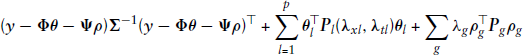
using appropriate penalty matrices ${\mathbf{P}}_l({\mathbf{\lambda }}_{\mathit{xl}},{\mathbf{\lambda }}_{\mathit{tl}})$ and ${\mathbf{P}}_g$ for the fixed effects and random effects, respectively, and smoothing parameters ${\mathbf{\lambda }}_{\mathit{xl}}=\left({\lambda }_{\mathit{xl}}^{(1)},...,{\lambda }_{\mathit{xl}}^{(D)}\right),{\mathbf{\lambda }}_{\mathit{tl}}=\left({\lambda }_{\mathit{tl}}^{(1)},...,{\lambda }_{\mathit{tl}}^{(D)}\right)$ , and ${\lambda }_g$ . The model and penalty matrices as well as the parameter vectors of (3.4) and (3.5) are discussed in detail below.

3.2.2 Modelling of fixed effects

The block-diagonal matrix $\mathbf{\Phi }=\mathrm{diag}\left({\mathbf{\Phi }}^{(1)},...,{\mathbf{\Phi }}^{(D)}\right)$ models the fixed effects separately on each dimension as in a FAMM (Scheipl et al., 2015). The $(\mathit{DNT}\times b)$ matrix $\mathbf{\Phi }$ consists of the design matrices ${\mathbf{\Phi }}^{(d)}=({\mathbf{\Phi }}_1^{(d)}|...|{\mathbf{\Phi }}_p^{(d)})$ that are constructed for the partial predictors $f_l^{(d)}(\mathbf{x},{\mathbf{t}}^{(d)}),l=1,...,p$ , which correspond to the $\mathit{NT}$ -vectors of evaluations of the effect functions $f_l^{(d)}$ . The vectors of scalar covariates ${\mathbf{x}}_i$ are repeated $T$ times to form the matrix of covariate information $\mathbf{x}=({\mathbf{x}}_1,...,{\mathbf{x}}_1,...,{\mathbf{x}}_N{)}^{\top }$ . We use the basis representations

$$\begin{array}{cc}{f}_l^{(d)}(\mathbf{x},{\mathbf{t}}^{(d)})\approx {\mathbf{\Phi }}_l^{(d)}{\mathbf{\theta }}_l^{(d)}=({\mathbf{\Phi }}_{\mathit{xl}}^{(d)}\odot {\mathbf{\Phi }}_{\mathit{tl}}^{(d)}){\mathbf{\theta }}_l^{(d)},\hfill & \hfill \end{array}$$

where $\mathbf{A}\odot \mathbf{B}$ denotes the row tensor product $(\mathbf{A}\otimes 1_b^{\top })·(1_a^{\top }\otimes \mathbf{B})$ of the $(h\times a)$ matrix $\mathbf{A}$ and the $(h\times b)$ matrix $\mathbf{B}$ with element-wise multiplication $·$ and $1_c$ the $c$ -vector of ones. This modelling approach combines the $(\mathit{NT}\times b_{\mathit{xl}}^{(d)})$ basis matrix ${\mathbf{\Phi }}_{\mathit{xl}}^{(d)}$ with the $(\mathit{NT}\times b_{\mathit{tl}}^{(d)})$ basis matrix ${\mathbf{\Phi }}_{\mathit{tl}}^{(d)}$ . These matrices contain the evaluations of suitable marginal bases in $\mathbf{x}$ and ${\mathbf{t}}^{(d)}$ , respectively. For a linear effect, for example, the basis matrix ${\mathbf{\Phi }}_{\mathit{xl}}^{(d)}$ is specified as the familiar linear model design matrix $\mathbf{x}$ for the linear effect $f_l^{(d)}(\mathbf{x},{\mathbf{t}}^{(d)})=\mathbf{x}{\mathbf{\beta }}_l^{(d)}({\mathbf{t}}^{(d)})$ with coefficient function ${\mathbf{\beta }}_l^{(d)}({\mathbf{t}}^{(d)})$ . For a nonlinear effect $f_l^{(d)}(\mathbf{x},{\mathbf{t}}^{(d)})=g_l^{(d)}(\mathbf{x},{\mathbf{t}}^{(d)})$ , the basis matrix ${\mathbf{\Phi }}_{\mathit{xl}}^{(d)}$ contains an (e.g., B-spline) basis representation analogously to a scalar additive model. For the functional intercept, ${\mathbf{\Phi }}_{\mathit{xl}}^{(d)}$ is a vector of ones, and we generally use a spline basis for ${\mathbf{\Phi }}_{\mathit{tl}}^{(d)}$ . For a complete list of possible effect specifications with examples, we refer to Scheipl et al. (2015). The tensor product basis is weighted by the $b_{\mathit{xl}}^{(d)}{b}_{\mathit{tl}}^{(d)}$ unknown basis coefficients in ${\mathbf{\theta }}_l^{(d)}$ . Stacking the vectors ${\mathbf{\theta }}_l^{(d)}$ gives ${\mathbf{\theta }}^{(d)}=({\mathbf{\theta }}_1^{(d)\top },...,{\mathbf{\theta }}_p^{(d)\top }{)}^{\top }$ and finally the $b$ -vector $\mathbf{\theta }=({\mathbf{\theta }}^{(1)\top },...,{\mathbf{\theta }}^{(D)\top }{)}^{\top }$ with $b={\sum }_d{\sum }_l{b}_{\mathit{xl}}^{(d)}{b}_{\mathit{tl}}^{(d)}$ .

Choosing the number of basis functions is a well known challenge in the estimation of nonlinear or functional effects. We introduce regularization by a corresponding quadratic penalty term in (3.5). Let ${\mathbf{\theta }}_l$ contain the coefficients corresponding to the partial predictor $l$ and order it by dimensions. The penalty ${\mathbf{P}}_l({\mathbf{\lambda }}_{\mathit{xl}},{\mathbf{\lambda }}_{\mathit{tl}})$ is then constructed from the penalty on the marginal basis for the covariate effect, ${\mathbf{P}}_{\mathit{xl}}^{(d)}$ , and the penalty on the marginal basis over the functional index, ${\mathbf{P}}_{\mathit{tl}}^{(d)}$ . Specifically, ${\mathbf{P}}_l({\mathbf{\lambda }}_{\mathit{xl}},{\mathbf{\lambda }}_{\mathit{tl}})$ is a block-diagonal matrix with blocks for each $d$ corresponding to the Kronecker sums of the marginal penalty matrices ${\lambda }_{\mathit{xl}}^{(d)}{\mathbf{P}}_{\mathit{xl}}^{(d)}\otimes {\mathbf{I}}_{b_{\mathit{tl}}^{(d)}}+{\lambda }_{\mathit{tl}}^{(d)}{\mathbf{I}}_{b_{\mathit{xl}}^{(d)}}\otimes {\mathbf{P}}_{\mathit{tl}}^{(d)}$ (Wood, 2017). A standard choice for these marginal penalty matrices given a B-splines basis representation are second or third order difference penalties, thus approximately penalizing squared second or third derivatives of the respective functions (Eilers and Marx, 1996). For unpenalized effects such as a linear effect of a scalar covariate, the corresponding ${\mathbf{P}}_{\mathit{xl}}^{(d)}$ is simply a matrix of zeroes.

3.2.3 Modelling of random effects

We represent the $\mathit{DNT}$ -vectors ${\mathbf{U}}_j(\mathbf{t})=({\mathbf{U}}_j({\mathbf{t}}^{(1)}{)}^{\top },...,{\mathbf{U}}_j({\mathbf{t}}^{(D)}{)}^{\top }{)}^{\top }$ , $\mathbf{E}(\mathbf{t})=(\mathbf{E}({\mathbf{t}}^{(1)}{)}^{\top },...,\mathbf{E}({\mathbf{t}}^{(D)}{)}^{\top }{)}^{\top }$ with ${\mathbf{U}}_j({\mathbf{t}}^{(d)})$ , $\mathbf{E}({\mathbf{t}}^{(d)})$ containing the evaluations of the univariate random effects for the corresponding groups and time points using the basis approximations

$$\begin{array}{cc}{\mathbf{U}}_j(\mathbf{t})\approx {\mathbf{\Psi }}_{U_j}{\mathbf{\rho }}_{U_j}=({\mathbf{\delta }}_{U_j}\odot {\tilde{\mathbf{\Psi }}}_{U_j}){\mathbf{\rho }}_{U_j},\mathbf{E}(\mathbf{t})\approx {\mathbf{\Psi }}_E{\mathbf{\rho }}_E=({\mathbf{\delta }}_E\odot {\tilde{\mathbf{\Psi }}}_E){\mathbf{\rho }}_E.\hfill & \hfill \end{array}$$

The $v$ th column in the $(\mathit{DNT}\times V_g),g\in \{U_1,...,U_q,E\}$ indicator matrix ${\mathbf{\delta }}_g$ indicates whether a given row is from the $v$ th group of the corresponding grouping layer. Thus, the rows of the indicator matrix ${\mathbf{\delta }}_g$ contain repetitions of the group indicators ${\mathbf{z}}_{\mathit{ij}}^{\top }$ and ${\mathbf{e}}_i^{\top }$ in model (2.1). For the smooth residual, ${\mathbf{\delta }}_E$ simplifies to $1_D\otimes ({\mathbf{I}}_N\otimes 1_T)$ . The $(\mathit{DNT}\times M_g)$ matrix ${\tilde{\mathbf{\Psi }}}_g=({\tilde{\mathbf{\Psi }}}_g^{(1)\top }|...|{\tilde{\mathbf{\Psi }}}_g^{(D)\top }{)}^{\top }$ comprises the evaluations of the $M_g$ multivariate eigenfunctions ${\psi }_{\mathit{gm}}^{(d)}(t)$ on dimensions $d=1,...,D$ for the $\mathit{NT}$ time points contained in the $(\mathit{NT}\times M_g)$ matrix ${\tilde{\mathbf{\Psi }}}_g^{(d)}$ . The $M_g{V}_g$ vector ${\mathbf{\rho }}_g=({\mathbf{\rho }}_{g1}^{\top },...,{\mathbf{\rho }}_{{\mathit{gV}}_g}^{\top }{)}^{\top }$ with ${\mathbf{\rho }}_{\mathit{gv}}=({\rho }_{\mathit{gv}1},...,{\rho }_{{\mathit{gvM}}_g}{)}^{\top }$ stacks all the unknown random scores for the functional random effect $g$ . The $(\mathit{DNT}\times {\sum }_g{M}_g{V}_g)$ model matrix $\mathbf{\Psi }=({\mathbf{\Psi }}_{U_1}|...|{\mathbf{\Psi }}_{U_q}|{\mathbf{\Psi }}_E)$ then combines all random effect design matrices. Stacking the vectors of random scores in a ${\sum }_g{M}_g{V}_g$ vector $\mathbf{\rho }=({\mathbf{\rho }}_{U_1}^{\top },...,{\mathbf{\rho }}_{U_q}^{\top },{\mathbf{\rho }}_E^{\top }{)}^{\top }$ lets us represent all functional random intercepts in the model via $\mathbf{\Psi }\mathbf{\rho }$ .

For a given functional random effect, the penalty takes the form ${\mathbf{\rho }}_g^{\top }{\mathbf{P}}_g{\mathbf{\rho }}_g={\mathbf{\rho }}_g^{\top }({\mathbf{I}}_{V_g}\otimes {\tilde{\mathbf{P}}}_g){\mathbf{\rho }}_g$ , where ${\mathbf{I}}_{V_g}$ corresponds to the assumed independence between the $V_g$ different groups. The diagonal matrix ${\tilde{\mathbf{P}}}_g=\mathrm{diag}({\nu }_{g1},...,{\nu }_{{\mathit{gM}}_g}{)}^{-1}$ contains the (estimated) eigenvalues ${\nu }_{\mathit{gm}}$ of the associated multivariate FPCs. This quadratic penalty is mathematically equivalent to a normal distribution assumption on the scores ${\mathbf{\rho }}_{\mathit{gv}}$ with mean zero and covariance matrix ${\tilde{\mathbf{P}}}_g^{-1}$ , as implied by the KL theorem for Gaussian random processes. Note that the smoothing parameter ${\lambda }_g$ allows for additional scaling of the covariance of the corresponding random process.

3.2.4 Estimation

We estimate the unknown smoothing parameters in ${\mathbf{\lambda }}_{\mathit{xl}},{\mathbf{\lambda }}_{\mathit{tl}}$ , and ${\lambda }_g$ using fast restricted maximum likelihood (REML)-estimation (Wood, 2017). The standard identifiability constraints of FAMMs are used (Scheipl et al., 2015). In particular, in addition to the constraints for the fixed effects, the multivariate random intercepts are subject to a sum-to-zero constraint over all evaluation points as given by, for example, Goldsmith et al. (2016).

We propose a weighted regression approach to handle the heteroscedasticity assumption contained in $\mathbf{\Sigma }$ . We weigh each observation proportionally to the inverse of the estimated univariate measurement error variances ${\widehat{\sigma }}_d^2$ from the estimation of the univariate covariances (3.2). Alternatively, updated measurement error variances can be obtained from fitting separate univariate FAMMs on the dimensions using the univariate components of the multivariate FPCs basis. In practice, we found that the less computationally intensive former option gives reasonable results.

As our proposed model is part of the FAMM framework, inference for the multiFAMM is readily available based on inference for scalar additive mixed models (Wood, 2017). Note, however, that all inferential statements do not incorporate uncertainty due to the estimated multivariate eigenfunction bases, nor in the chosen smoothing parameters. The estimation process readily provides, amongst other things, standard errors for the construction of point-wise univariate confidence bands (CBs).

3.3 Implementation

We provide an implementation of the estimation of the proposed multiFAMM in the multifamm R-package (Volkmann, 2021). It is possible to include up to two functional random intercepts in $\mathbf{U}(t)$ , which can have a nested or crossed structure, in addition to the curve-specific random intercept ${\mathbf{E}}_i(t)$ . While including, for example, functional covariates is conceptually straightforward (see Scheipl et al., 2015), our implementation is restricted to scalar covariates and interactions thereof. We provide different alternatives for specifying the multivariate scalar product, the multivariate cut-off criterion, and the covariance matrix of the white noise error term. Note that the estimated univariate error variances have been proposed as weights for two separate and independent modelling decisions: as weights in the scalar product of the MFPCA and as regression weights under heteroscedasticity across dimensions.

4 Applications

We illustrate the proposed multiFAMM for two different data applications corresponding to intrinsically multivariate and multimodal fuctional data. The presentation focuses on the first application with a detailed description of the multimodal data application in Supplementary Material C. We provide the data and the code to produce all analyses in the Supplementary Material (http://www.statmod.org/smij/archive.html).

4.1 Snooker training data

4.1.1 Data set and preprocessing

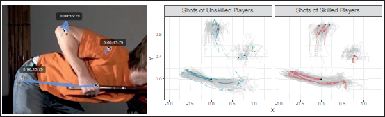
In a study by Enghofer (2014), 25 recreational snooker players split into two groups, one of which had instructions to follow a self-administered training schedule over the next six weeks consisting of exercises aimed at improving snooker specific muscular coordination. The second was a control group. Before and after the training period, both groups were recorded on high-speed digital camera under similar conditions to investigate the effects of the training on their snooker shot of maximal force. In each of the two recording sessions, six successful shots per participant were videotaped. The recordings were then used to manually locate points of interest (a participant's shoulder, elbow, and hand) and track them on a two-dimensional grid over the course of the video. This yields a six-dimensional functional observation per snooker shot ${\mathbf{y}}^{*}=(y^{*(\mathit{elbow}.\mathit{x})},...,y^{*(\mathit{shoulder}.\mathit{y})}):\mathcal{I}=[0,1]\to {\mathbb{ℝ}}^6$ , that is, a two-dimensional movement trajectory for each point of interest (see Figure 1).

Figure 1

Screenshot of software for tracking (lines) the points of interest (circles) (left), two-dimensional trajectories of the snooker training data set (grey curves, right). For both groups of skilled and unskilled participants, three randomly selected observations are highlighted and every line type corresponds to one multivariate observation, that is, one observation consists of three trajectories: elbow (top), shoulder (right) and hand (bottom). The start of the exemplary trajectories are marked with a black asterisk with the hand trajectory centred at the origin

In their starting position (hand centred at the origin), the snooker players are positioned centrally in front of the snooker table aiming at the cue ball. From their starting position, the players draw back the cue, then accelerate it forwards and hit the cue ball shortly after their hands enter the positive range of the horizontal $x$ -axis. After the impulse onto the cue ball, the hand movement continues until it is stopped at a player's chest. Enghofer (2014) identify two underlying techniques that a player can apply: dynamic and fixed elbow. With a dynamic elbow, the cue can be moved in an almost straight line (piston stroke) whereas additionally fixing the elbow results in a pendular motion (pendulum stroke). In both cases, the shoulder serves as a fixed point and should be positioned close to the snooker table.

We adjust the data for differences in body height and relative speed (Steyer et al., 2021) and apply a coarsening method to reduce the number of redundant data points, thereby lowering computational demands of the analysis. Supplementary Material B provides a detailed description of the data preprocessing. As some recordings and evaluations of bivariate trajectories are missing, the final dataset contains 295 functional observations with a total of 56,910 evaluation points. These multivariate functional data are irregular and sparse, with a median of 30 evaluation points per functional observation (minimum 8, maximum 80) for each of the six dimensions.

4.1.2 Model specification

We estimate the following model

$$\begin{array}{cc}{\mathbf{y}}_{\mathit{ijht}}=\mathbf{\mu }({\mathbf{x}}_{\mathit{ij}},t)+{\mathbf{B}}_i(t)+{\mathbf{C}}_{\mathit{ij}}(t)+{\mathbf{E}}_{\mathit{ijh}}(t)+{\mathbf{\epsilon }}_{\mathit{ijht}},\hfill & \hfill \end{array}$$

(4.1)

with $i=1,...,25$ the index for the snooker player, $j=1,2$ the index for the session, $h=1,...,H_{\mathit{ij}}$ the index for the typically six snooker shot repetitions in a session, and $t\in [0,1]$ relative time. Correspondingly, ${\mathbf{B}}_i(t)$ is a subject-specific random intercept, ${\mathbf{C}}_{\mathit{ij}}(t)$ is a nested subject-and-session-specific random intercept, and ${\mathbf{E}}_{\mathit{ijh}}(t)$ is the shot-specific random intercept (smooth residual). The nested random effect ${\mathbf{C}}_{\mathit{ij}}(t)$ is supposed to capture the variation within players between sessions (e.g., differences due to players having a good or bad day). Different positioning of participants with respect to the recording equipment or the snooker table as well as shot to shot variation are captured by the smooth residual ${\mathbf{E}}_{\mathit{ijh}}(t)$ . The white noise measurement error ${\mathbf{\epsilon }}_{\mathit{ijht}}$ is assumed to follow a zero-mean multivariate normal distribution with covariance matrix ${\sigma }^2{\mathbf{I}}_6$ , as all six dimensions are measured with the same set-up. The additive predictor is defined as

$$\begin{array}{cc}\mathbf{\mu }({\mathbf{x}}_{\mathit{ij}},t)\hfill & ={\mathbf{f}}_0(t)+{\mathtt{skill}}_i·{\mathbf{f}}_1(t)+{\mathtt{group}}_i·{\mathbf{f}}_2(t)+{\mathtt{session}}_j·{\mathbf{f}}_3(t)\hfill \\ \hfill & +{\mathtt{group}}_i·{\mathtt{session}}_j·{\mathbf{f}}_4(t).\hfill \end{array}$$

The dummy covariates ${\mathtt{skill}}_i$ and ${\mathtt{group}}_i$ indicate whether player $i$ is an advanced snooker player and belongs to the treatment group (i.e., receives the training programme), respectively. Note that the snooker players self-select into training and control group to improve compliance with the training programme, which is why we include a group effect in the model. The dummy covariate ${\mathtt{session}}_j$ indicates whether the shot $j$ is recorded after the training period. The effect function ${\mathbf{f}}_4(t)$ can thus be interpreted as the treatment effect of the training programme.

Cubic P-splines with first-order difference penalty, penalizing deviations from constant functions over time, with 8 basis functions are used for all effect functions in the preliminary mean estimation as well as in the final multiFAMM. For the estimation of the auto-covariances of the random processes, we use cubic P-splines with first-order difference penalty on five marginal basis functions. We use an unweighted scalar product (3.3) for the MFPCA to give equal weight to all spatial dimensions, as we can assume that the measurement error mechanism is similar across dimensions. Additionally, we find that hand, elbow, and shoulder contribute roughly the same amount of variation to the data, cf. Table 1 in Supplementary Material B.3, where we also discuss potential weighting schemes for the MFPCA. The multivariate truncation order is chosen such that 95% of the (unweighted) sum of variation (3.4) is explained.

4.1.3 Results

The MFPCA gives sets of five (for $\mathbf{C}$ and $\mathbf{E}$ ) and six (for $\mathbf{B}$ ) multivariate FPCs that explain 95% of the total variation. The estimated eigenvalues allow to quantify their relative importance. Approximately 41% of the total variation (conditional on covariates) can be attributed to the nested subject-and-session-specific random intercept ${\mathbf{C}}_{\mathit{ij}}(t)$ , 33% to the subject-specific random intercept ${\mathbf{B}}_i(t)$ , 14% to the shot-specific ${\mathbf{E}}_{\mathit{ijh}}(t)$ , and 7% to white noise. This suggests that day to day variation within a snooker player is larger than the variation between snooker players. Note that these proportions are based on estimation step 1 (see Section 3.1).

Figure 2

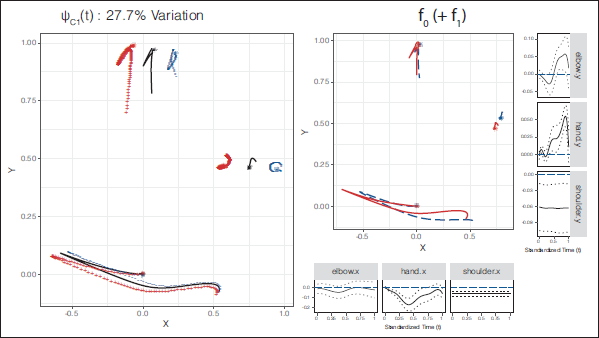
Dominant mode ( ${\mathbf{\psi }}_{C1}$ ) of the subject-and-session-specific random effect, explaining $27.7\%$ of total variation and shown as mean trajectory (black solid) plus ( $+$ ) or minus ( $-$ ) $2\sqrt{{\nu }_{C1}}$ times the first FPCs (left). An asterisk marks the start of a trajectory. Estimated covariate effect functions for skill (right). The central plot shows the effect of the coefficient function (solid) on the two-dimensional trajectories for the reference group (dashed). The marginal plots show the estimated univariate effect functions (solid) with pointwise 95% CBs (dotted) and the baseline (dashed)

The left plot of Figure 2 displays the first FPC for $\mathbf{C}$ , which explains about $28\%$ of total variation. A suitable multiple of the FPCs is added ( $+$ ) to and subtracted ( $-$ ) from the overall mean function (black solid line, all covariate values set to $0.5$ ). We find that the dominant mode of the random subject-and-session-specific effect influences the relative positioning of a player's elbow, shoulder, and hand, thus suggesting a strong dependence between the dimensions. Enghofer (2014) argue from a theoretical viewpoint that the ideal starting position should place elbow and hand in a line perpendicular to the plane of the snooker table (corresponding to the x-axis). The most prominent mode of variation captures deviations from this ideal starting position found in the overall mean. The next most important FPC ${\mathbf{\psi }}_{B1}$ of the subject-specific random effect, which explains about $15\%$ of total variation, represents a subject's tendency towards the piston or pendulum stroke (see Supplementary Material Figure 4). This additional insight into the underlying structure of the variance components might be helpful for, for example, developing personalized training programmes.

The central plot on the right of Figure 2 compares the estimated mean movement trajectory for advanced snooker players (solid line) to that in the reference group (dashed). It suggests that more experienced players tend towards the dynamic elbow technique, generating a hand trajectory resembling a straight line (piston stroke). Uncertainties in the trajectory could be represented by pointwise ellipses, but inference is more straightforward to obtain from the univariate effect functions. The marginal plots display the estimated univariate effects with pointwise 95% confidence intervals. Even though we find only little statistical evidence for increased movement of the elbow (horizontal-left and vertical-top marginal panels), the hand and shoulder movements (horizontal centre and right, vertical centre and bottom) strongly suggest that the skill level indeed influences the mean movement trajectory of a snooker player. Further results indicate that the mean hand trajectories might slightly differ between treatment and control group at baseline as well as between sessions ( ${\mathbf{f}}_2(t)$ and ${\mathbf{f}}_3(t)$ , see Supplementary Material Figure 8). The estimated treatment effect ${\mathbf{f}}_4(t)$ (Supplementary Material Figure 7), however, suggests that the training programme did not change the participants’ mean movement trajectories substantially. Supplementary Material B.3 contains a detailed discussion of all model terms as well as some model diagnostics and sensitivity analyses.

4.2 Consonant assimilation data

4.2.1 Data set and model specification

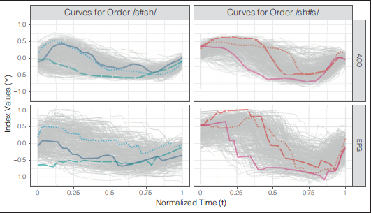
Pouplier and Hoole (2016) study the assimilation of the German /s/ and /sh/ sounds such as the final consonant sounds in ‘Kürbis’ (English example: ‘haggis’) and ‘Gemisch’ (English example: ‘dish’), respectively. The research question is how these sounds assimilate in fluent speech when combined across words such as in ‘Kürbis-Schale’ or ‘Gemisch-Salbe’, denoted as /s#sh/ and /sh#s/ with # the word boundary. The 9 native German speakers in the study repeated a set of 16 selected word combinations five times. Two different types of functional data, that is, (ACO) and electropalatographic (EPG) data, were recorded for each repetition to capture the acoustic (produced sound) and articulatory (tongue movements) aspects of assimilation over (relative) time $t$ within the consonant combination.

Each functional index varies roughly between $+1$ and $-1$ and measures how similar the articulatory or acoustic pattern is to its reference patterns for the first ( $+1$ ) and second ( $-1$ ) consonant at every observed time point (Cederbaum et al., 2016). Without assimilation, the data are thus expected to shift from positive to negative values in a sinus-like form (see Figure 3). The dataset contains 707 bivariate functional observations with differently spaced grids of evaluation points per curve and dimension, with the number of evaluation points ranging from 22 to 59 with a median of 35. Note that the consonant assimilation data are unaligned as registration of the time domain would mask transition speeds between the consonants, which are an interesting part of assimilation.

Figure 3

Index curves of the consonant assimilation dataset for both ACO and EPG data as a function of standardized time $t$ (grey curves). For every consonant order, three randomly selected observations have been highlighted and every line type corresponds to one multivariate observation, that is, one observation consists of two index curves

For comparability, we follow the model specification of Cederbaum et al. (2016), who analyse only the ACO dimension and ignore the second mode EPG. Our specified multivariate model is similar to (4.1) with $i=1,...,9$ the speaker index, $j=1,...,16$ the word combination index, $h=1,...,H_{\mathit{ij}}$ the repetition index and $t\in [0,1]$ relative time. Note that the nested effect ${\mathbf{C}}_{\mathit{ij}}(t)$ is replaced by the crossed random effect ${\mathbf{C}}_j(t)$ specific to the word combinations. The additive predictor $\mathbf{\mu }({\mathbf{x}}_j,t)$ now contains eight partial effects: the functional intercept plus main and interaction effects of scalar covariates describing characteristics of the word combination such as the order of the consonants /s/ and /sh/. The white noise measurement error ${\mathbf{\epsilon }}_{\mathit{ijht}}$ is assumed to follow a zero-mean bivariate normal distribution with diagonal covariance matrix $\mathrm{diag}({\sigma }_{\mathit{ACO}}^2,{\sigma }_{\mathit{EPG}}^2)$ . The basis and penalty specifications follow the univariate analysis in Cederbaum et al. (2016). Given different sampling mechanisms, we also compare the multiFAMM based on weighted and unweighted scalar products for the MFPCA.

4.2.2 Results

The multivariate analysis supports the findings of Cederbaum et al. (2016) that assimilation is asymmetric (different mean patterns for /s#sh/ and /sh#s/). Overall, the estimated fixed effects are similar across dimensions as well as comparable to the univariate analysis. Hence, the multivariate analysis indicates that previous results for the acoustics are consistently found also for the articulation. Compared to univariate analyses, our approach reduces the number of FPC basis functions and thus the number of parameters in the analysis. The multiFAMM can improve the model fit and can provide smaller CBs for the ACO dimension compared to the univariate model in Cederbaum et al. (2016) due to the strong cross-correlation between the dimensions. We find similar modes of variation for the multivariate and the univariate analysis as well as across dimensions. In particular, the word combination-specific random effect ${\mathbf{C}}_j(t)$ is dropped from the model as much of the between-word variation is already explained by the included fixed effects. The definition of the scalar product has little effect on the estimated fixed effects but changes the interpretation of the FPCs. Supplementary Material C contains a more in-depth description of this application.

5 Simulations

5.1 Simulation set-up

We conduct an extensive simulation study to investigate the performance of the multiFAMM depending on different model specifications and data settings (over 20 scenarios total), and to compare it to univariate regression models as proposed by Cederbaum et al. (2016), estimated on each dimension independently. Given the broad scope of analysed model scenarios, we refer the interested reader to Supplementary Material D for a detailed report and restrict the presentation here to the main results.

We mimic our two presented data examples (Section 4) and simulate new data based on the respective multiFAMM-fit. Each scenario consists of model fits to 500 generated datasets, where we randomly draw the number and location of the evaluation points, the random scores, and the measurement errors according to different data settings. The accuracy of the estimated model components is measured by the root relative mean squared error (rrMSE) based on the unweighted multivariate norm but otherwise as defined by Cederbaum et al. (2016), see Supplementary Material D.1. The rrMSE takes on (unbounded) positive values with smaller values indicating a better fit.

5.2 Simulation results

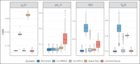
Figure 4 compares the rrMSE values over selected modelling scenarios based on the consonant assimilation data. We generate a benchmark scenario (far left boxplots), which imitates the original data without misspecification of any model component. In particular, the number of FPCs is fixed to avoid truncation effects. Comparing this scenario to the two scenarios left and centre illustrates the importance of the number of FPCs in the accuracy of the estimation. Choosing the truncation order via the proportion of univariate variance explained (Cut-Off Uni) as in (3.5) gives models with roughly the same number of FPCs (mean $\mathbf{B}:2.8,\mathbf{E}:5$ ) as is used for the data generation ( $\mathbf{B}:3,\mathbf{E}:5$ ). The cut-off criterion based on the multivariate variance (Cut-Off Mul) given by (3.4) results in more parsimonious models (mean $\mathbf{B}:2.15,\mathbf{E}:4$ ) and thus considerably higher rrMSE values. The increased variation in the rrMSE values can also be attributed to variability in the truncation orders (cf. Supplementary Material Figure 19), leading to a mixture distribution. Comparing the benchmark scenario to more sparsely observed functional data (ceteris paribus) suggests a lower estimation accuracy for the Sparse Data scenario (right), especially for the curve-specific random effect ${\mathbf{E}}_{\mathit{ijh}}(t)$ and resultingly the fitted curves ${\mathbf{y}}_{\mathit{ijh}}(t)$ , but pooling the information across functions helps the estimation of $\mathbf{\mu }({\mathbf{x}}_{\mathit{ij}},t)$ and ${\mathbf{B}}_i(t)$ . In particular, the estimation of the mean $\mathbf{\mu }({\mathbf{x}}_{\mathit{ij}},t)$ is quite robust against the increased uncertainty of these three scenarios. Only when the random scores are not centred and decorrelated as in the benchmark scenario do we find an increase in rrMSE values for the mean (Uncentred Scores, far right). This corresponds to a departure from the modelling assumptions likely to occur in practice when only few levels of a random effect are available (here for the subject-specific ${\mathbf{B}}_i(t)$ ). The model then has difficulties to correctly separate the intercept in $\mathbf{\mu }({\mathbf{x}}_{\mathit{ij}},t)$ and the random effects ${\mathbf{B}}_i(t)$ . The empirical (non-zero) mean of the ${\mathbf{B}}_i(t)$ is then absorbed by the intercept in $\mathbf{\mu }({\mathbf{x}}_{\mathit{ij}},t)$ , resulting in higher rrMSE values for both of these model terms. However, this shift does not affect the overall fit to the data ${\mathbf{y}}_{\mathit{ijh}}(t)$ nor the estimation of the other fixed effects (cf. Supplementary Material Figure 27). Note that the rrMSE values of the Sparse Data and Uncentred Scores scenarios are based on slightly different normalizing constants (i.e., different true data) and cannot be directly compared except for the mean.

Figure 4

rrMSE values of the fitted curves ${\mathbf{y}}_{\mathit{ijh}}(t)$ , the mean $\mathbf{\mu }({\mathbf{x}}_{\mathit{ij}},t)$ , and the random effects ${\mathbf{B}}_i(t)$ and ${\mathbf{E}}_{\mathit{ijh}}(t)$ for different modelling scenarios. The three leftmost scenarios correspond to different model specifications in the same data setting

Our simulation study thus suggests that basing the truncation orders on the proportion of explained variation on each dimension (3.5) gives parsimonious and well-fitting models. If interest lies mainly in the estimation of fixed effects, the alternative cut-off criterion based on the total variation in the data (3.4) allows even more parsimonious models at the cost of a less accurate estimation of the random effects and overall model fit. Furthermore, the results presented in Supplementary Material D show that the mean estimation is relatively stable over different model scenarios including misspecification of the measurement error variance structure or of the multivariate scalar product, as well as in scenarios with strong heteroscedasticity across dimensions. In our benchmark scenario, the CBs cover the true effect $89-94\%$ of the time but coverage can further decrease with additional uncertainty, for example, about the number of FPCs. Overall, the covariance structure such as the leading FPCs can be recovered well, also for a nested random effect such as in the snooker training application. The comparison to the univariate modelling approach suggests that the multiFAMM can improve the mean estimation but is especially beneficial for the prediction of the random effects while reducing the number of parameters to estimate. In some cases like strong heteroscedasticity, including weights in the multivariate scalar product might further improve the modelling.

6 Discussion

The proposed multivariate functional regression model is an additive mixed model, which allows to model flexible covariate effects for sparse or irregular multivariate functional data. It uses FPC based functional random effects to model complex correlations within and between functions and dimensions. An important contribution of our approach is estimating the parsimonious multivariate FPC basis from the data. This allows us to account not only for auto-covariances, but also for non-trivial cross-covariances over dimensions, which are difficult to adequately model using alternative approaches such as parametric covariance functions like the Matèrn family or penalized splines, which imply a parsimonious covariance only within but not necessarily between functions. As a FAMM-type regression model, a wide range of covariate effect types is available, also providing pointwise CBs. Our applications show that the multiFAMMs can give valuable insight into the multivariate correlation structure of the functions in addition to the mean structure.

An apparent benefit of multivariate modelling is that it allows to answer research questions simultaneously relating to different dimensions. In addition, using multivariate FPCs reduces the number of parameters compared to fitting comparable univariate models while improving the random effects estimation by incorporating the cross-covariance in the multivariate analysis. The added computational costs are small: For our multimodal application, the multivariate approach prolongs the computation time by only 5% (104 vs. 109 minutes on a 64-bit Linux platform).

We find that the average point-wise coverage of the point-wise CBs can in some cases lie considerably below the nominal value. There are two main reasons for this: One, the CBs presented here do not incorporate the uncertainty of the eigenfunction estimation nor of the smoothing parameter selection. Two, coverage issues can arise in (scalar) mixed models, if effect functions are estimated as constant when in truth they are not (e.g., Wood, 2017; Greven and Scheipl, 2016). To resolve these issues, further research on the level of scalar mixed models might be needed. A large body of research covering CB estimation for functional data (e.g., Goldsmith et al., 2013; Choi and Reimherr, 2018; Liebl and Reimherr, 2019) suggests that the construction of CBs is an interesting and complex problem, also outside of the FAMM framework.

It would be interesting to extend the multiFAMM to more general scenarios of multivariate functional data such as observations consisting of functions with different dimensional domains, for example, functions over time and images as in Happ and Greven (2018). This would require adapting the estimation of the univariate auto-covariances for spatial arguments $t,t^{\prime }$ . Exploiting properties of dense functional data, such as the block structure of design matrices for functions observed on a grid, could help to reduce computational cost in this case. Future research could further generalize the covariance structure of the multiFAMM by allowing for additional covariate effects. In our snooker training application, for example, a treatment effect of the snooker training might show itself in the form of reduced intra-player variance (cf. Backenroth et al., 2018). Ideas from distributional regression could be incorporated to jointly model the mean trajectories and covariance structure conditional on covariates.