Assessing intra- and inter-method agreement of functional data

Abstract

Modern medical devices are increasingly producing complex data that could offer deeper insights into physiological mechanisms of underlying diseases. One type of complex data that arises frequently in medical imaging studies is functional data, whose sampling unit is a smooth continuous function. In this work, with the goal of establishing the scientific validity of experiments involving modern medical imaging devices, we focus on the problem of evaluating reliability and reproducibility of multiple functional data that are measured on the same subjects by different methods (i.e. different technologies or raters). Specifically, we develop a series of intraclass correlation coefficient and concordance correlation coefficient indices that can assess intra-method, inter-method, and total (intra + inter) agreement based on multivariate multilevel functional data consisting of replicated functional data measurements produced by each of the different methods. For efficient estimation, the proposed indices are expressed using variance components of a multivariate multilevel functional mixed effect model, which can be smoothly estimated by functional principal component analysis. Extensive simulation studies are performed to assess the finite-sample properties of the estimators. The proposed method is applied to evaluate the reliability and reproducibility of renogram curves produced by a high-tech radionuclide image scan used to non-invasively detect kidney obstruction.

1. Introduction

In biomedical studies, clinical measurements provide an objective means of diagnosing, monitoring, or refuting a patient’s physiological condition, state of health, and disease. The recent advancement in technology has led to introduction of many new clinical measurement scales that could potentially offer deeper insights into disease and pathological mechanisms. To ensure that scientific conclusions derived from a new clinical measurement scale are trustworthy, it is necessary to evaluate its reliability and reproducibility. From a statistical standpoint, this amounts to assessing agreement among target clinical measurements produced by several methods, technologies, or raters on a common subject/unit. ¹

Various statistical methods have been developed to assess agreement among multiple methods when clinical measurements are continuous. Intraclass correlation coefficient (ICC) is one of the popular measures of agreement for continuous measurements.^2,3 Let $X_{ij}$ denote the clinical measurement of the $i$ th subject produced by the $j$ th method ( $i=1,\dots ,n$ ; $j=1,\dots ,J$ ). The ICC is based on the following linear mixed model:

$$X_{ij}=\mu +{\alpha }_i+{ϵ}_{ij}$$

where fixed effect $\mu$ denotes the grand mean of the measurements over all methods, ${\alpha }_i$ is a random subject effect with mean zero and variance ${\sigma }_{\alpha }^2$ , and ${ϵ}_{ij}$ denotes a random interaction effect between rater and subject with mean zero and variance ${\sigma }_{ϵ}^2$ . Then assuming ${\alpha }_i$ and ${ϵ}_{ij}$ are uncorrelated, the ICC is defined as

$$\begin{array}{r}\mathrm{ICC}=\frac{{\sigma }_{\alpha }^2}{{\sigma }_{\alpha }^2+{\sigma }_{ϵ}^2}\end{array}$$

(1)

The index is scaled between 0 and 1, and the closer the index value is to 1, the better the agreement among different methods. One major limitation of ICC is that it assumes measurements produced by different methods share the common mean and variance (the exchangeable assumption), which is often not true in practice.

Concordance correlation coefficient (CCC) is another popular measure of agreement for continuous readings.^4,5 The basic idea is to quantify the degree of concordance among measurements from $J$ methods by the sum of their pairwise expected squared differences $\sum _{j=1}^{J-1}\sum _{j^{\prime }=j+1}^J\text{E}(X_{ij}-X_{i{j}^{\prime }}{)}^2$ . Then the index is constructed by scaling $\sum _{j=1}^{J-1}\sum _{j^{\prime }=j+1}^J\text{E}(X_{ij}-X_{i{j}^{\prime }}{)}^2$ by its counterpart under the assumption that all methods are independent; that is,

$$\begin{array}{rl}\mathrm{CCC}& =1-\frac{\sum _{j=1}^{J-1}\sum _{j^{\prime }=j+1}^J\text{E}(X_{ij}-X_{i{j}^{\prime }}{)}^2}{\sum _{j=1}^{J-1}\sum _{j^{\prime }=j+1}^J{\text{E}}_I(X_{ij}-X_{i{j}^{\prime }}{)}^2}\\ & =\frac{2\sum _{j=1}^{J-1}\sum _{j^{\prime }=j+1}^J{\sigma }_{j{j}^{\prime }}}{\sum _{j=1}^{J-1}\sum _{j^{\prime }=j+1}^J({\mu }_j-{\mu }_{j^{\prime }}{)}^2+(J-1)\sum _{j=1}^J{\sigma }_j^2}\end{array}$$

where ${\text{E}}_I$ denotes the expectation conditional on the assumption that $X_{ij}$ and $X_{i{j}^{\prime }}$ are independent, $\text{E}(X_{ij})={\mu }_j,\text{Var}(X_{ij})={\sigma }_j^2$ and $\text{Cov}(X_{ij},X_{i{j}^{\prime }})={\sigma }_{j{j}^{\prime }}$ . A value of $1(-1)$ denotes perfect concordance (discordance); a value of zero denotes no concordance. Unlike the ICC, no statistical model is assumed, and measurements from different methods can have different means and variances. Several extensions of CCC have been proposed to assess agreement under different contexts: a weighted CCC for a repeated measures design, ⁶ a robust version of the CCC, ⁷ and a series of indices (intra-ICC, inter-CCC, and total-CCC) that can assess intra-method, inter-method, and total (inter $+$ intra) agreement when there are replicated readings taken by each of the multiple methods on a given subject. ⁷

With advancements in technology, modern medical devices are increasingly producing complex data that could offer deeper insights into physiological mechanisms underlying diseases and aid in improving diagnostic capabilities. One such type of data that arises frequently in medical imaging studies is functional data, whose sampling unit is a smooth continuous function defined over a time, space, or other continuum. To date, many functional data analysis methods have been developed to analyze functional data and translate their rich structural information into clinically useful applications. ⁸

However, there is limited work on the development of statistical methods for assessing agreement of functional data measurements. One ad hoc approach to evaluate agreement of functional data is to compute pointwise ICCs or CCCs across the time points. This approach, however, produces highly variable (non-smooth) ICC or CCC curves that are hard to interpret and not applicable to irregular functional data. An alternative naive approach is to project the functions on the space spanned by a set of pre-specified basis functions (e.g. B-splines, Fourier basis, wavelets, etc.) and extract the corresponding basis coefficients as low-dimensional representations of the functions. Then, treating the extracted basis coefficients as continuous readings, one can compute the existing ICC and CCC indices ⁷ to assess intra-method, inter-method, and total agreement. This approach, however, has two major drawbacks: (i) the pre-specified set of basis functions may not capture important aspects of the data, resulting in loss of information; and (ii) a loss of efficiency occurs as smoothing of functions is done for each observational unit independently, without borrowing information from other observations. Another approach utilizing a weighted CCC ⁶ for repeated measures is not appropriate for functional data because observation for each subject is very dense, more like a set of curves over time rather than a multi-dimensional vector of repeated measurements.

More recently, three approaches that are specifically tailored to assess agreement of functional data were introduced. Initially, an extended CCC index that can assess agreement between functional data produced by two different methods was proposed. ⁹ The index is defined based on a modified inner product in some probability functional space and is estimated via a method of moments. Next, an extended ICC index that is appropriate for assessing the agreement of images (two-dimensional functions) was developed. ¹⁰ Here, the index is formulated based on the traces of variance component operators—which are extensions of ${\sigma }_{\alpha }^2$ and ${\sigma }_{ϵ}^2$ in (1) to the functional space—and are estimated based on multilevel functional principal component analysis (FPCA) . ¹¹ More recently, a functional CCC index that can evaluate agreement of functional data produced by two or more different methods was introduced. ¹² To facilitate parsimonious modeling and stable estimation of the index, the method utilizes multivariate FPCA ¹³ to represent the measurements using a small number of method-specific principal components. Unlike the first two extended CCC ⁹ and ICC ¹⁰ indices, this functional CCC itself is a function of time and provides insight into how the degree of agreement changes over time.

The aforementioned agreement studies for functional data, however, assume that only one functional data measurement is produced by each method on a single subject. The problem here is that the index formulated under such a design can only evaluate total agreement that contains both intra- and inter-method agreement, without being able to separate the two. In order to assess intra-method, inter-method, and total agreement separately, a development of a series of ICC and CCC indices formulated under a design with replicated functional data measurements from each of the several methods on each subject (i.e. multivariate multilevel functional data) is required but has not yet been pursued; our article aims to fill this important gap.

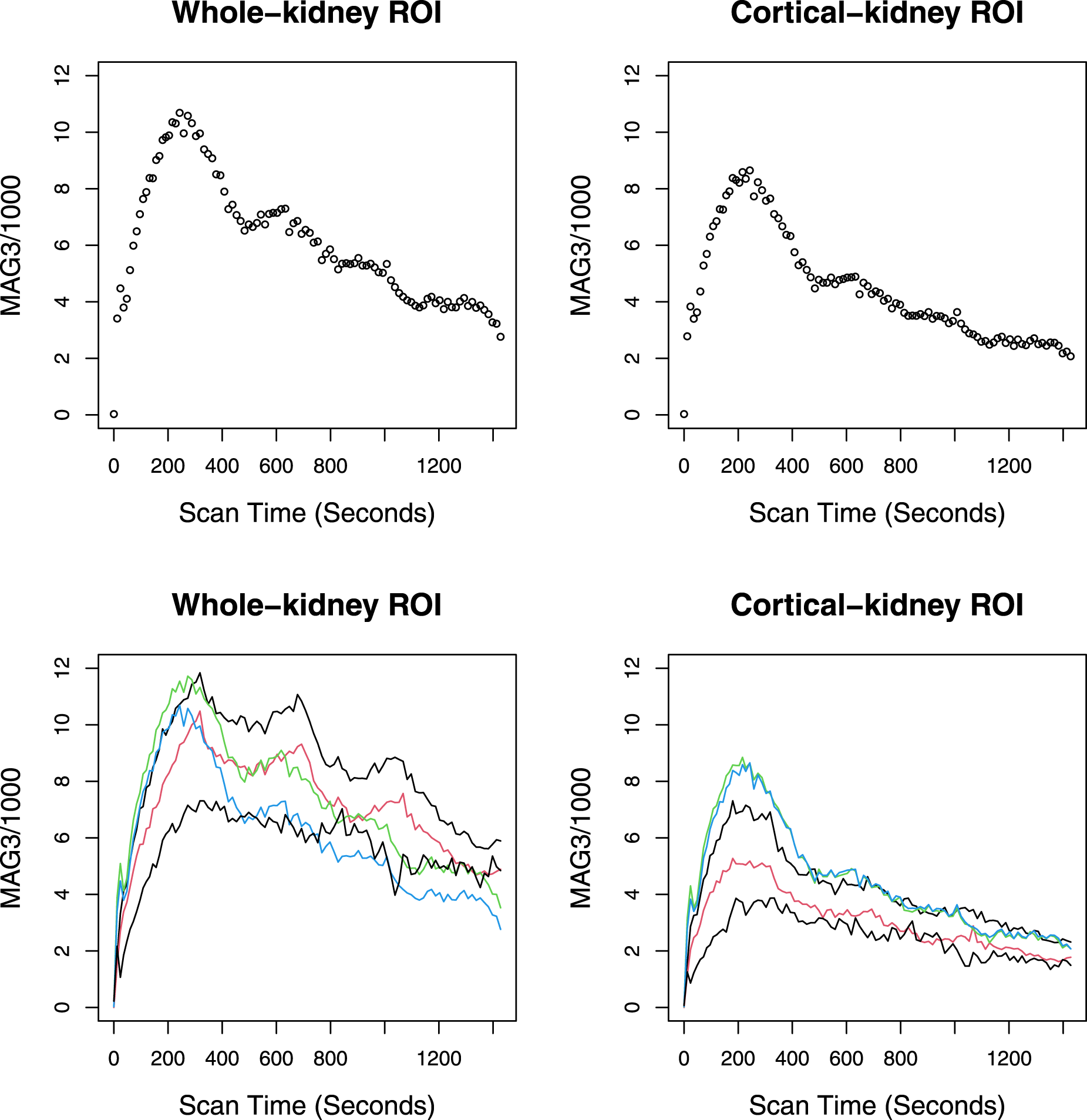
Our work is motivated by the renal study conducted at Emory University. One of the study goals is to evaluate the reliability and reproducibility of a high-tech medical imaging device called Technetium-99m mercaptoacetyltriglycine (MAG3) renography, which is widely used to non-invasively detect kidney obstruction. ¹⁴ The data collection experiment begins with an intravenous injection of MAG3, a gamma-emitting tracer, that is absorbed by the kidneys and then travels down the ureters from the kidney to the bladder. During the process, the MAG3 photons are imaged and quantified on a user-defined region of interest (ROI) in the kidney, and a renogram curve, which represents the MAG3 photon counts detected at 100 time points (every 12–15 s) during a period of 1428 s on the ROI, is produced. There are two methods for specifying the ROI in the kidney. In the first method, a radiologist specifies an ROI within a whole region of the kidney and is called a “whole-kidney ROI method.” In the second method, a radiologist focuses exclusively on the outer layer of the kidney (renal cortex), where the nephrons begin, and specifies an ROI within it; this method is called the “cortical-kidney ROI method.” The top panel of Figure 1 shows renogram curves (with time-varying MAG3 photon counts expressed as dots) produced by the whole-kidney ROI method (left panel) and the cortical-kidney ROI method (right panel) on a representative kidney in the data set. The bottom panel simultaneously presents the renogram curves of five selected kidneys from the data set.

Figure 1.

The top panel presents the renogram curves (dots representing the series of MAG3 photon counts/1000 quantified over 1428 s) produced by the whole-kidney ROI method (left panel) and the cortical-kidney ROI method (right panel) on a representative kidney from the Emory renal study data set. The bottom panel presents the renogram curves of five selected kidneys in the data set. MAG3: mercaptoacetyltriglycine; ROI: region of interest.

The specific research question pertaining to the evaluation of the reliability and reproducibility of MAG3 renography is two-fold. First, are the renogram curves produced by each of the methods on the same kidney reproducible across multiple ROI specification attempts by the practicing radiologist? Investigating this question by assessing intra-method agreement can help establish the reliability of clinical measurements produced by MAG3 renography for detecting and monitoring kidney obstruction. Second, is the renogram curve produced by one method reproducible by another method (inter-method agreement)? If so, the diagnostic procedure can be simplified as a practicing radiologist can focus on interpreting a renogram curve produced by one of the two methods.

To answer these research questions, we develop a set of ICC and CCC indices that can assess intra-method, inter-method, and total agreement of functional data measurements. Two types of indices are proposed. The first type consists of “time-dependent” ICC and CCC indices that can quantify degree of agreement varying smoothly over time. These time-dependent indices are particularly useful for cases where identifying a subset of the domain with high agreement or delineating the trend of agreement is of interest. The second type comprises “global” indices that summarize agreement over the entire time domain using a single measure.

We use a model-based approach for defining and estimating the indices. Specifically, we begin by formulating a multivariate multilevel functional mixed effects model, under which functional data measurements produced by multiple methods are written as a sum of multivariate grand mean function, subject-specific random effect function, and residual subject- and replication-specific random effect function. Such a formulation allows us to write the indices as functions of within- and between-subject variance components, which in turn can be expressed as truncated multivariate Karhunen–Loéve (KL) expansions. This leads to the following three-step procedure for estimating the indices: (i) we estimate the terms (scores, eigenvalues, and eigenfunctions) of the univariate multilevel KL expansion based on the univariate multilevel FPCA ¹¹ and then combine them in a way that produces the consistent estimates for the terms of the multivariate multilevel KL expansion; (ii) use the estimated terms of the multivariate multilevel KL expansion to produce the estimates of within- and between-subject variance components; and (iii) use the estimated variance components to produce the estimates of the indices. For inference, we propose to construct the confidence bands and intervals of the indices based on an non-parametric bootstrap at the subject level.

The remainder of the article is organized as follows. In Section 2, we first introduce a multivariate multilevel functional mixed effects model for functional data measurements produced by multiple methods. We then introduce ICC and CCC indices for assessing intra-method, inter-method, and total agreement of functional data and provide an efficient estimation strategy based on FPCA. In Section 3, we conduct simulation studies to evaluate the performance of the proposed approach. The application of our methods to the Emory renal study is described in Section 4. Concluding remarks are in Section 5.

2. Methods

2.1. Data object

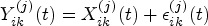
Let $X_{ik}^{(j)}(t)$ denote a $k$ th replication of a square-integrable random function measured over a continuous variable $t\in \mathcal{T}$ by method $j$ on subject $i$ for $k=1,\dots ,K$ , $j=1,\dots J$ and $i=1,\dots ,n$ . In our application, a function $X$ denotes a renogram curve, $t$ is a renal scan time, $\mathcal{T}=[0,1428]$ is a renal scan period (in seconds), $i$ is a kidney, and $j$ stands for either a “whole-kidney ROI method” ( $j=1)$ or “cortical-kidney ROI method” ( $j=2)$ .

Combining the functions across different methods for each replicate and subject, we obtain the multivariate functional object ${\mathbf{X}}_{ik}(t)=(X_{ik}^{(1)}(t),\dots ,X_{ik}^{(J)}(t){)}^{\mathrm{\top }}$ with the multivariate mean function

$$\mathit{\mu }(t)={({\mu }^{(1)}(t),\dots ,{\mu }^{(J)}(t))}^{\mathrm{\top }}={(\text{E}\{X_{ik}^{(1)}(t)\},\dots ,\text{E}\{X_{ik}^{(J)}(t)\})}^{\mathrm{\top }}$$

for all $t\in \mathcal{T}$ . For $s,t\in \mathcal{T}$ , the matrix of total covariance functions is defined as ${\mathbf{C}}_T(s,t):=\text{E}[\{{\mathbf{X}}_{ik}(s)-\mathit{\mu }(s)\}\otimes \{{\mathbf{X}}_{ik}(t)-\mathit{\mu }(t)\}$ , whose $j$ th row and $h$ th column ( $j,h=1,\dots ,J$ ) element is

$$C_T^{(jh)}(s,t)=\text{Cov}\{X_{ik}^{(j)}(s),X_{ik}^{(h)}(t)\}=\text{E}\left[\{X_{ik}^{(j)}(s)-{\mu }^{(j)}(s)\}\{X_{ik}^{(h)}(t)-{\mu }^{(h)}(t)\}\right]$$

For $k,q=1,\dots ,K$ , the matrix of covariance function between the replicates within the same subject is defined as ${\mathbf{C}}_B(s,t):=\text{E}[\{{\mathbf{X}}_{ik}(s)-\mathit{\mu }(s)\}\otimes \{{\mathbf{X}}_{iq}(t)-\mathit{\mu }(t)\}$ , whose $j$ th row and $h$ th column element is

$$C_B^{(jh)}(s,t)=\text{Cov}\{X_{ik}^{(j)}(s),X_{iq}^{(h)}(t)\}=\text{E}\left[\{X_{ik}^{(j)}(s)-{\mu }^{(j)}(s)\}\{X_{iq}^{(h)}(t)-{\mu }^{(h)}(t)\}\right]$$

Note that ${\mathbf{C}}_B(s,t)$ does not depend on $k$ and $q$ , implying that the common covariance structure is imposed between any pair of replicates.

2.2. Modeling of data

We introduce the following multivariate multilevel functional mixed effects model for the agreement analysis:

$$\begin{array}{r}{\mathbf{X}}_{ik}(t)=\mathit{\mu }(t)+{\mathbf{Z}}_i(t)+{\mathbf{W}}_{ik}(t),t\in \mathcal{T}\end{array}$$

(2)

where ${\mathbf{Z}}_i(t)=(Z_i^{(1)}(t),\dots ,Z_i^{(J)}(t){)}^{\mathrm{\top }}$ is the subject-specific random effect function (level 1 function), and ${\mathbf{W}}_{ik}=(W_{ik}^{(1)}(t),\dots ,W_{ik}^{(J)}(t){)}^{\mathrm{\top }}$ is the residual subject- and replication-specific random effect function (level 2 function). This model is a multivariate extension of the two-way functional analysis of variance model ¹¹ and a multilevel extension of the uncentered multivariate KL expansion. ¹⁵ We make the following assumptions for the model: (a) $\mathit{\mu }(t)$ is a fixed function; (b) each $Z_i^{(j)}(t)$ is a mean zero stochastic process with between-subject variance ${\sigma }_{Bj}^2(t)=\text{Var}\{Z_i^{(j)}(t)\}$ ; (c) each $W_{ik}^{(j)}(t)$ is a mean zero stochastic process with within-subject variance ${\sigma }_{Wj}^2(t)=\text{Var}\{W_{ik}^{(j)}(t)\}$ ; (d) $Z_i^{(j)}(t)$ ’s are correlated across the methods with ${\sigma }_{j{j}^{\prime }}(t)=\text{Cov}\{Z_i^{(j)}(t),Z_i^{(j^{\prime })}(t)\}$ ; (e) $W_{ik}^{(j)}(t)$ ’s are independent across the replicates and methods; and (e) ${\mathbf{Z}}_i(t)$ and ${\mathbf{W}}_{ik}(t)$ are mutually uncorrelated.

To facilitate the estimation of the variance components ${\sigma }_{Bj}^2(t)$ , ${\sigma }_{Wj}^2(t)$ , and ${\sigma }_{j{j}^{\prime }}(t)$ , which constitute the agreement measures introduced in the next section, we decompose both level 1 and level 2 functions in (2) based on the following multivariate multilevel KL expansion

$$\begin{array}{r}{\mathbf{Z}}_i(t)=\sum _{m=1}^{\mathrm{\infty }}{\zeta }_{im}^{[1]}{\mathit{\psi }}_m^{[1]}(t)\text{and}{\mathbf{W}}_{ik}(t)=\sum _{l=1}^{\mathrm{\infty }}{\zeta }_{ikl}^{[2]}{\mathit{\psi }}_l^{[2]}(t)\end{array}$$

(3)

Here, for $m\in \mathbb{N}$ , ${\mathit{\psi }}_m^{[1]}(t)=({\psi }_m^{[1](1)}(t),\dots ,{\psi }_m^{[1](J)}(t){)}^{\mathrm{\top }}$ are level 1 multivariate eigenfunctions corresponding to the non-decreasing eigenvalues ${\lambda }_m^{[1]}$ from the spectral decomposition of the “between” covariance function: ${\mathbf{C}}_B(s,t)=\sum _{m=1}^{\mathrm{\infty }}{\lambda }_m^{[1]}{\mathit{\psi }}_m^{[1]}(s){\mathit{\psi }}_m^{[1]}(t)$ . Note that $\{{\mathit{\psi }}_m^{[1]}(t):m=1,2,\dots \}$ forms an orthonormal basis of the space of multivariate functions $\mathcal{F}=\{L^2(\mathcal{T}){\}}^J$ ; that is, $\sum _{j=1}^J{\int }_{\mathcal{T}}{\psi }_{m_1}^{[1](j)}(t){\psi }_{m_2}^{[1](j)}(t)dt=\mathbb{I}(m_1=m_2)$ . The coefficients ${\zeta }_{im}^{[1]}$ are random variables (called level 1 scores) with $\text{E}({\zeta }_{im}^{[1]})=0$ , $\text{Var}({\zeta }_{im}^{[1]})={\lambda }_m^{[1]}$ and $\text{E}({\zeta }_{im}^{[1]}{\zeta }_{i{m}^{\prime }}^{[1]})=0$ for any $m\ne m^{\prime }$ . For $l\in \mathbb{N}$ , ${\mathit{\psi }}_l^{[2]}(t)=({\psi }_l^{[2](1)}(t),\dots {\psi }_l^{[2](J)}(t){)}^{\mathrm{\top }}$ are level 2 multivariate eigenfunctions corresponding to the non-decreasing eigenvalues ${\lambda }_l^{[2]}$ from the spectral decomposition ${\mathbf{C}}_W(s,t)=\sum _{l=1}^{\mathrm{\infty }}{\lambda }_l{\mathit{\psi }}_l^{[2]}(s){\mathit{\psi }}_l^{[2]}(t)$ , where ${\mathbf{C}}_W(s,t):={\mathbf{C}}_T(s,t)-{\mathbf{C}}_B(s,t)$ . The set $\{{\mathit{\psi }}_l^{[2]}(t):l=1,2,\dots \}$ also forms an orthonormal basis of $\mathcal{F}$ , and the coefficients ${\zeta }_{ikl}^{[2]}$ are level 2 scores with $\text{E}({\zeta }_{ikl}^{[2]})=0$ , $\text{Var}({\zeta }_{ikl}^{[2]})={\lambda }_l^{[2]}$ , and $\text{E}({\zeta }_{ikl}^{[2]}{\zeta }_{ik{l}^{\prime }}^{[2]})=0$ for any $l\ne l^{\prime }$ . We further assume that $\{{\zeta }_{im}^{[1]}:m=1,2,\dots \}$ are uncorrelated with $\{{\zeta }_{ikl}^{[2]}:l=1,2,\dots \}$ .

Model (2) with the multivariate multilevel KL expansion (3) becomes

$${\mathbf{X}}_{ik}(t)=\mathit{\mu }(t)+\sum _{m=1}^{\mathrm{\infty }}{\zeta }_{im}^{[1]}{\mathit{\psi }}_m^{[1]}(t)+\sum _{l=1}^{\mathrm{\infty }}{\zeta }_{ikl}^{[2]}{\mathit{\psi }}_l^{[2]}(t),t\in \mathcal{T}$$

which gives the following expressions for the variance components of main interest:

$$\begin{array}{r}\begin{array}{rl}& {\sigma }_{Bj}^2(t)=\sum _{m=1}^{\mathrm{\infty }}{\lambda }_m^{[1]}\{{\psi }_m^{[1](j)}(t){\}}^2,{\sigma }_{Wj}^2(t)=\sum _{l=1}^{\mathrm{\infty }}{\lambda }_l^{[2]}\{{\psi }_l^{[2](j)}(t){\}}^2,\text{and}\\ & {\sigma }_{j{j}^{\prime }}(t)=\sum _{m=1}^{\mathrm{\infty }}{\lambda }_m^{[1]}{\psi }_m^{[1](j)}(t){\psi }_m^{[1](j^{\prime })}(t)\end{array}\end{array}$$

(4)

for $j,j^{\prime }=1,\dots ,J$ , and $t\in \mathcal{T}$ .

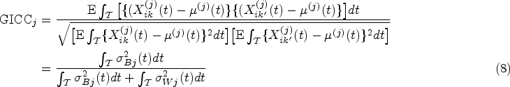
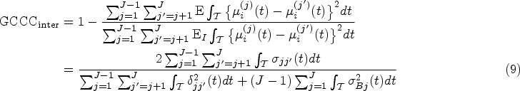
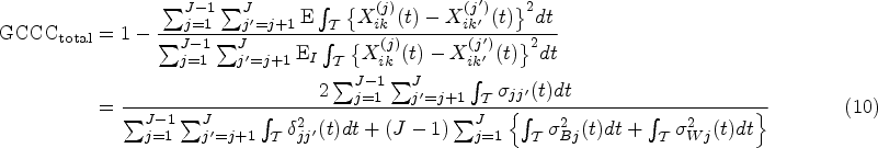
2.3. Agreement measures

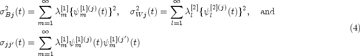
Based on the multivariate multilevel functional mixed effects model (2), we introduce three types of agreement indices for functional data: (i) ICC that measures agreement among repetitions of a single method (intra-method agreement); (ii) inter-CCC that quantifies agreement among different methods based on the true readings of each method without replication error (inter-method agreement); and (iii) total-CCC that measures total (intra $+$ inter) agreement based on any observed individual reading from each method. We first introduce a “time-dependent” version of the indices, which quantifies the degree of agreement varying smoothly over time $t$ . These time-dependent indices are particularly useful for cases where identifying a subset of the domain with high agreement or delineating the trend of agreement is of interest.

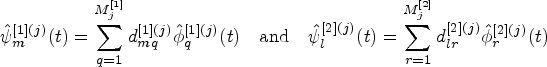
For a given method, say $j$ , we have $\text{E}\{X_{ik}^{(j)}(t)\}={\mu }^{(j)}(t)$ and $\text{Var}\{X_{ik}^{(j)}(t)\}={\sigma }_{Bj}^2(t)+{\sigma }_{Wj}^2(t)$ for any $k$ under model (2); that is, the replicates of a given method are interchangeable. As such, the following ICC index can be used to quantify the degree of concordance between the replicated readings of method $j$ at each time point $t$ (intra-method agreement):

$$\begin{array}{r}{\mathrm{ICC}}_j(t)=\frac{\text{Cov}\{X_{ik}^{(j)}(t),X_{i{k}^{\prime }}^{(j)}(t)\}}{\sqrt{\text{Var}\{X_{ik}^{(j)}(t)\}\text{Var}\{X_{i{k}^{\prime }}^{(j)}(t)\}}}=\frac{{\sigma }_{Bj}^2(t)}{{\sigma }_{Bj}^2(t)+{\sigma }_{Wj}^2(t)}\end{array}$$

(5)

For each method, the ICC measures the proportion of variance that is attributable to the subjects, and it is heavily dependent on the total variability (total data range).

At each $t$ , the inter-CCC quantifies the degree of concordance among different methods (inter-method agreement) based on the true readings of each method, ${\mu }_i^{(j)}(t)={\mu }^{(j)}(t)+Z_i^{(j)}(t)$ , which are not obscured by the within-method replication error:

$$\begin{array}{r}\begin{array}{rl}{\mathrm{CCC}}_{\mathrm{inter}}(t)& =1-\frac{\sum _{j=1}^{J-1}\sum _{j^{\prime }=j+1}^J\text{E}\{{\mu }_i^{(j)}(t)-{\mu }_i^{(j^{\prime })}(t){\}}^2}{\sum _{j=1}^{J-1}\sum _{j^{\prime }=j+1}^J{\text{E}}_I\{{\mu }_i^{(j)}(t)-{\mu }_i^{(j^{\prime })}(t){\}}^2}\\ & =\frac{2\sum _{j=1}^{J-1}\sum _{j^{\prime }=j+1}^J{\sigma }_{j{j}^{\prime }}(t)}{\sum _{j=1}^{J-1}\sum _{j^{\prime }=j+1}^J{\delta }_{j{j}^{\prime }}^2(t)+(J-1)\sum _{j=1}^J{\sigma }_{Bj}^2(t)}\end{array}\end{array}$$

(6)

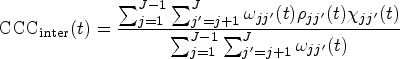
Here, ${\text{E}}_I$ denotes the expectation conditional on the assumption that ${\mu }_i^{(j)}(t)$ and ${\mu }_i^{(j^{\prime })}(t)$ are independent, and ${\delta }_{j{j}^{\prime }}(t)={\mu }^{(j)}(t)-{\mu }^{(j^{\prime })}(t)$ . Note that the inter-CCC depends on the between-subject variability ${\sigma }_{Bj}^2(t)$ but not on the within-subject variance ${\sigma }_{Wj}^2(t)$ , thus capturing the pure agreement among the methods while effectively denoising the intra-method differences. Note that we can rewrite the inter-CCC (6) as

$${\mathrm{CCC}}_{\mathrm{inter}}(t)=\frac{\sum _{j=1}^{J-1}\sum _{j^{\prime }=j+1}^J{\omega }_{j{j}^{\prime }}(t){\rho }_{j{j}^{\prime }}(t){\chi }_{j{j}^{\prime }}(t)}{\sum _{j=1}^{J-1}\sum _{j^{\prime }=j+1}^J{\omega }_{j{j}^{\prime }}(t)}$$

where ${\omega }_{j{j}^{\prime }}(t)={\delta }_{j{j}^{\prime }}^2(t)+{\sigma }_{Bj}^2(t)+{\sigma }_{B{j}^{\prime }}^2(t)$ , ${\rho }_{j{j}^{\prime }}(t)={\sigma }_{j{j}^{\prime }}(t)/\{{\sigma }_{Bj}(t){\sigma }_{B{j}^{\prime }}(t)\}$ , and ${\chi }_{j{j}^{\prime }}(t)=2{\sigma }_{Bj}(t){\sigma }_{B{j}^{\prime }}(t)/{\omega }_{j{j}^{\prime }}=[\{v_{j{j}^{\prime }}(t)+1/v_{j{j}^{\prime }}(t)+u_{j{j}^{\prime }}^2(t)\}/2{]}^{-1}$ , with $v_{j{j}^{\prime }}(t)={\sigma }_{Bj}(t)/{\sigma }_{B{j}^{\prime }}(t)$ and $u_{j{j}^{\prime }}(t)={\delta }_{j{j}^{\prime }}(t)/\{{\sigma }_{Bj}(t){\sigma }_{B{j}^{\prime }}(t){\}}^{1/2}$ . Here, ${\rho }_{j{j}^{\prime }}(t)$ denotes Pearson’s correlation coefficient representing the degree of “precision” between methods $j$ and $j^{\prime }$ . The degree of “accuracy” between the two methods is quantified by ${\chi }_{j{j}^{\prime }}(t)$ , which contains $v_{j{j}^{\prime }}(t)$ representing scale shift and $u_{j{j}^{\prime }}(t)$ representing location shift relative to the scale.^4,16 This formulation allows us to investigate the source of disagreement between a particular pair of methods. That is, a low value of ${\rho }_{j{j}^{\prime }}(t)$ implies that the disagreement is due to lack of precision, while high values of $v_{j{j}^{\prime }}(t)$ and $u_{j{j}^{\prime }}(t)$ suggest that the disagreement is due to scale shift and location shift, respectively.

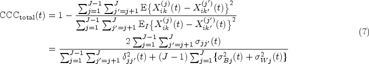
The total CCC quantifies the total agreement containing both intra-method agreement and inter-method agreement. The index is formulated based on any individual reading from each method, given that the replicated readings from the same method are independently and identically distributed (iid). Thus, the total CCC does not depend on the number of replicates and is defined as

$$\begin{array}{r}\begin{array}{rl}{\mathrm{CCC}}_{\mathrm{total}}(t)& =1-\frac{\sum _{j=1}^{J-1}\sum _{j^{\prime }=j+1}^J\text{E}\{X_{ik}^{(j)}(t)-X_{i{k}^{\prime }}^{(j^{\prime })}(t){\}}^2}{\sum _{j=1}^{J-1}\sum _{j^{\prime }=j+1}^J{\text{E}}_I\{X_{ik}^{(j)}(t)-X_{i{k}^{\prime }}^{(j^{\prime })}(t){\}}^2}\\ & =\frac{2\sum _{j=1}^{J-1}\sum _{j^{\prime }=j+1}^J{\sigma }_{j{j}^{\prime }}(t)}{\sum _{j=1}^{J-1}\sum _{j^{\prime }=j+1}^J{\delta }_{j{j}^{\prime }}^2(t)+(J-1)\sum _{j=1}^J\{{\sigma }_{Bj}^2(t)+{\sigma }_{Wj}^2(t)\}}\end{array}\end{array}$$

(7)

where ${\text{E}}_I$ denotes the expectation conditional on the assumption that $X_{ik}^{(j)}(t)$ and $X_{i{k}^{\prime }}^{(j)}(t)$ are independent. Note that the total CCC, which is defined at the level of observed readings, consists of both ${\sigma }_{Bj}^2(t)$ and ${\sigma }_{Wj}^2(t)$ ; that is, the index takes into account both the intra- and inter-method variabilities in the readings for assessing agreement.

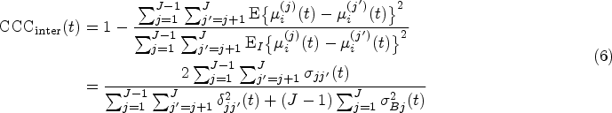
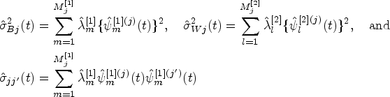
In some cases, we may be interested in the “global” agreement measure that summarizes the agreement of functional data over the entire domain $\mathcal{T}$ . The following agreement indices, global ICC ( ${\mathrm{GICC}}_j$ ), global inter-CCC ( ${\mathrm{GCCC}}_{\mathrm{inter}}$ ) and global total-CCC ( ${\mathrm{GCCC}}_{\mathrm{total}}$ ), respectively, summarize the intra-method, inter-method, and total agreement of functional data over their entire domain $\mathcal{T}$ :

$$\begin{array}{rl}{\mathrm{GICC}}_j& =\frac{\text{E}{\int }_{\mathcal{T}}[\{(X_{ik}^{(j)}(t)-{\mu }^{(j)}(t)\}\{(X_{i{k}^{\prime }}^{(j)}(t)-{\mu }^{(j)}(t)\}]dt}{\sqrt{[\text{E}{\int }_{\mathcal{T}}\{X_{ik}^{(j)}(t)-{\mu }^{(j)}(t){\}}^{2}dt][\text{E}{\int }_{\mathcal{T}}\{X_{i{k}^{\prime }}^{(j)}(t)-{\mu }^{(j)}(t){\}}^{2}dt]}}\\ & =\frac{{\int }_{\mathcal{T}}{\sigma }_{Bj}^2(t)dt}{{\int }_{\mathcal{T}}{\sigma }_{Bj}^2(t)dt+{\int }_{\mathcal{T}}{\sigma }_{Wj}^2(t)dt}\end{array}$$

(8)

$$\begin{array}{rl}{\mathrm{GCCC}}_{\mathrm{inter}}& =1-\frac{\sum _{j=1}^{J-1}\sum _{j^{\prime }=j+1}^J\text{E}{\int }_{\mathcal{T}}\{{\mu }_i^{(j)}(t)-{\mu }_i^{(j^{\prime })}(t){\}}^{2}dt}{\sum _{j=1}^{J-1}\sum _{j^{\prime }=j+1}^J{\text{E}}_I{\int }_{\mathcal{T}}\{{\mu }_i^{(j)}(t)-{\mu }_i^{(j^{\prime })}(t){\}}^{2}dt}\\ & =\frac{2\sum _{j=1}^{J-1}\sum _{j^{\prime }=j+1}^J{\int }_{\mathcal{T}}{\sigma }_{j{j}^{\prime }}(t)dt}{\sum _{j=1}^{J-1}\sum _{j^{\prime }=j+1}^J{\int }_{\mathcal{T}}{\delta }_{j{j}^{\prime }}^2(t)dt+(J-1)\sum _{j=1}^J{\int }_{\mathcal{T}}{\sigma }_{Bj}^2(t)dt}\end{array}$$

(9)

$$\begin{array}{rl}{\mathrm{GCCC}}_{\mathrm{total}}& =1-\frac{\sum _{j=1}^{J-1}\sum _{j^{\prime }=j+1}^J\text{E}{\int }_{\mathcal{T}}\{X_{ik}^{(j)}(t)-X_{i{k}^{\prime }}^{(j^{\prime })}(t){\}}^{2}dt}{\sum _{j=1}^{J-1}\sum _{j^{\prime }=j+1}^J{\text{E}}_I{\int }_{\mathcal{T}}\{X_{ik}^{(j)}(t)-X_{i{k}^{\prime }}^{(j^{\prime })}(t){\}}^{2}dt}\\ & =\frac{2\sum _{j=1}^{J-1}\sum _{j^{\prime }=j+1}^J{\int }_{\mathcal{T}}{\sigma }_{j{j}^{\prime }}(t)dt}{\sum _{j=1}^{J-1}\sum _{j^{\prime }=j+1}^J{\int }_{\mathcal{T}}{\delta }_{j{j}^{\prime }}^2(t)dt+(J-1)\sum _{j=1}^J\{{\int }_{\mathcal{T}}{\sigma }_{Bj}^2(t)dt+{\int }_{\mathcal{T}}{\sigma }_{Wj}^2(t)dt\}}\end{array}$$

(10)

Note that these indices are constructed using the moments based on the inner product $⟨X_1(.),X_2(.)⟩=\text{E}{\int }_{\mathcal{T}}{X}_1(t)X_2(t)dt$ , where $X_1(\cdot )$ and $X_2(\cdot )$ belong to a space of square-integrable random functions.

2.4. Estimation and inference

In this section, we introduce our approach for smoothly estimating the time-dependent indices (5)-(7) and estimating the global indices (8)-(10). Note that all indices are functions of the variance components ${\sigma }_{Bj}^2(t)$ , ${\sigma }_{Wj}^2(t)$ , and ${\sigma }_{j{j}^{\prime }}(t)$ , which, in turn, can be expressed as linear combinations of the KL expansion terms as in (4). Accordingly, the proposed estimation scheme comprises the following three steps.

The first step is to estimate the terms of the multivariate multilevel KL expansion (3), namely, ${\lambda }_m^{[1]}$ , ${\lambda }_l^{[2]}$ , ${\mathit{\psi }}_m^{[1]}(t)$ , and ${\mathit{\psi }}_l^{[2]}(t)$ (i.e. level 1 and 2 eigenvalues and multivariate eigenfunctions). To achieve this, we derive the univariate multilevel KL expansion of the level 1 and 2 functions in (2) separately for each $j$ th element as

$$\begin{array}{r}{Z}_i^{(j)}(t)=\sum _{m=1}^{\mathrm{\infty }}{\xi }_{im}^{[1](j)}{\varphi }_m^{[1](j)}(t)\text{and}{W}_{ik}^{(j)}(t)=\sum _{l=1}^{\mathrm{\infty }}{\xi }_{ikl}^{[2](j)}{\varphi }_l^{[2](j)}(t)\end{array}$$

(11)

Here, for $m\in \mathbb{N}$ , ${\varphi }_m^{[1](j)}(t)$ are level 1 univariate eigenfunctions corresponding to eigenvalues ${\tau }_m^{[1](j)}$ from the spectral decomposition $C_B^{(jj)}(s,t)=\text{Cov}\{X_{ik}^{(j)}(s),X_{iq}^{(j)}(t)\}=\sum _{m=1}^{\mathrm{\infty }}{\tau }_m^{[1](j)}{\varphi }_m^{[1](j)}(s){\varphi }_m^{[1](j)}(t)$ . The coefficients ${\xi }_{im}^{[1](j)}$ are mutually uncorrelated level 1 scores with $\text{E}({\xi }_{im}^{[1](j)})=0$ and $\text{Var}({\xi }_{im}^{[1](j)})={\tau }_m^{[1](j)}$ . For $l\in \mathbb{N}$ , ${\varphi }_l^{[2](j)}(t)$ are level 2 univariate eigenfunctions corresponding to eigenvalues ${\tau }_l^{[2](j)}$ from the spectral decomposition $C_W^{(jj)}(s,t)=\sum _{l=1}^{\mathrm{\infty }}{\tau }_l^{[2](j)}{\varphi }_l^{[2](j)}(s){\varphi }_l^{[2](j)}(t)$ , where $C_W^{(jj)}(s,t):=\text{Cov}\{X_{ik}^{(j)}(s),X_{ik}^{(j)}(t)\}-\text{Cov}\{X_{ik}^{(j)}(s),X_{iq}^{(j)}(t)\}$ . The coefficients ${\xi }_{ikl}^{[2](j)}$ are mutually uncorrelated level 2 scores with $\text{E}({\xi }_{ikl}^{[2](j)})=0$ and $\text{Var}({\xi }_{ikl}^{[2](j)})={\tau }_l^{[2](j)}$ . Note that the univariate multilevel KL expansion (11) uses information from readings of only one method (single $j$ ) at a time, while the multivariate counterpart (3) leverages information within and across different methods (multiple $j$ 's) simultaneously.

We now introduce an estimation framework based on FPCA that first estimates univariate multilevel KL expansion terms—namely, ${\varphi }_m^{[1](j)}(t)$ , ${\varphi }_l^{[2](j)}(t)$ , ${\tau }_m^{[1]}$ , ${\tau }_l^{[2]}$ , ${\xi }_{im}^{[1](j)}$ , and ${\xi }_{ikl}^{[2]}$ —and then combines them in a way that produces the estimates of the multivariate multilevel KL expansion terms ${\lambda }_m^{[1]}$ , ${\lambda }_l^{[2]}$ , ${\mathit{\psi }}_m^{[1]}$ , and ${\mathit{\psi }}_l^{[2]}(t)$ . The framework consists of the following four sub-steps.

In practice, each function $X_{ik}^{(j)}(t)$ is measured at a set of grid points $\{t_h:h=1,\dots ,T\}$ . Let $\{X_{ik}^{(j)}(t_h):i=1,\dots ,n,k=1,\dots ,K,h=1,\dots T\}$ denote the collection of observed readings of functional data produced by method $j$ . Perform univariate multilevel FPCA ¹¹ separately on data from each method to estimate the univariate KL expansion terms. That is, for each $j$ , obtain $\{{\hat{\varphi }}_m^{[1](j)}(t):m=1,\dots ,M_j^{[1]}\}$ , $\{{\hat{\varphi }}_l^{[2](j)}(t):l=1,\dots ,M_j^{[2]}\}$ , $\{{\hat{\tau }}_m^{[1](j)}:m=1,\dots ,M_j^{[1]}\}$ , $\{{\hat{\tau }}_l^{[2](j)}:l=1,\dots ,M_j^{[2]}\}$ , $\{{\hat{\xi }}_{im}^{[1](j)}:i=1,\dots ,n,m=1,\dots ,M_j^{[1]}\}$ , and $\{{\hat{\xi }}_{ikl}^{[2](j)},i=1,\dots ,n,k=1,\dots ,K,l=1,\dots ,M_j^{[2]}\}$ . Here, $M_j^{[v]}$ ( $v=1,2$ ) denote the optimal truncation lags for the univariate multivariate KL expansion (11), which can be chosen based on the percentage of variance explained; that is, $M_j^{[v]}=\underset{m}{min}\{(\sum _{u=1}^m{\hat{\tau }}_u^{[v](j)}/\sum _{u=1}^{T-1}{\hat{\tau }}_u^{[v](j)})>{\delta }_0\}$ such that the leading $M_j^{[v]}$ eigenfunctions explain $100{\delta }_0\mathrm{\%}$ (e.g. 90% or 95%) of total variability. Note that the univariate multilevel KL expansion terms are obtained based on the eigenanalyses of the univariate covariance functions estimated by the method of moments: ${\hat{C}}_T^{(jj)}(t_h,t_r)=(nK{)}^{-1}=\sum _{i,k}\{X_{ik}^{(j)}(t_h)-{\hat{\mu }}^{(j)}(t_h)\}\{X_{ik}^{(j)}(t_r)-{\hat{\mu }}^{(j)}(t_r)\}$ , ${\hat{C}}_B^{(jj)}(t_h,t_r)=2\{nK(K-1){\}}^{-1}\sum _i\sum _{k_1<k_2}\{X_{i{k}_1}^{(j)}(t_h)-{\hat{\mu }}^{(j)}(t_h)\}\{X_{i{k}_2}^{(j)}(t_r)-{\hat{\mu }}^{(j)}(t_r)\}$ , and ${\hat{C}}_W^{(jj)}(t_h,t_r)={\hat{C}}_T^{(jj)}(t_h,t_r)-{\hat{C}}_B^{(jj)}(t_h,t_r)$ , where ${\hat{\mu }}^{(j)}(t)=(nK{)}^{-1}\sum _{i,k}{X}_{ik}^{(j)}(t)$ . In many applications, functional data are observed with error (residual noise), that is

$$Y_{ik}^{(j)}(t)=X_{ik}^{(j)}(t)+{ϵ}_{ik}^{(j)}(t)$$

where ${ϵ}_{ik}^{(j)}(t)$ denotes the independent residual noise process with mean zero and variance ${\sigma }^2$ . There are three ways to handle error-prone functional data. The first approach is to smooth the data prior to applying the FPCA. ¹⁷ The second is to represent the functions using a set of basis functions (e.g. B-splines) and control their smoothness by introducing a penalty term. ¹⁸ The third is to smooth the covariance functions. ¹⁹ The detailed estimation procedure for the univariate multilevel FPCA based on the covariance smoothing approach is described in Section 2.3 of Di et al.’s paper. ¹¹

Let $M_{+}^{[v]}=\sum _{j=1}^J{M}_j^{[v]}$ ( $v=1,2$ ). Firstly, create the matrix ${\hat{\mathrm{\Xi }}}^{[1]}\in {\mathbb{R}}^{n\times M_{+}^{[1]}}$ , where each row $({\hat{\xi }}_{i1}^{[1](1)},\dots ,{\hat{\xi }}_{i,M_1^{[1]}}^{[1](1)},\dots ,{\hat{\xi }}_{i1}^{[1](J)},\dots ,{\hat{\xi }}_{i,M_J^{[1]}}^{[1](J)})$ contains all estimated level 1 scores for a single subject. Define ${\hat{\mathrm{\Sigma }}}^{[1]}=(n-1{)}^{-1}{\hat{\mathrm{\Xi }}}^{[1]\mathrm{\top }}{\hat{\mathrm{\Xi }}}^{[1]}$ . Secondly, create the matrix ${\hat{\mathrm{\Xi }}}^{[2]}\in {\mathbb{R}}^{nK\times M_{+}^{[2]}}$ , where each row $({\hat{\xi }}_{ik1}^{[2](1)},\dots ,{\hat{\xi }}_{ik,M_1^{[2]}}^{[2](1)},\dots ,{\hat{\xi }}_{ik1}^{[2](J)},\dots ,{\hat{\xi }}_{ik,M_J^{[2]}}^{[2](J)})$ contains all estimated level 2 scores for each replicate. Define ${\hat{\mathrm{\Sigma }}}^{[2]}=(nK-1{)}^{-1}{\hat{\mathrm{\Xi }}}^{[2]\mathrm{\top }}{\hat{\mathrm{\Xi }}}^{[2]}$ .

Firstly, perform an eigenanalysis of ${\hat{\mathrm{\Sigma }}}^{[1]}$ to obtain the eigenvalues ${\hat{\lambda }}_m^{[1]}$ of interest and the corresponding orthonormal eigenvectors ${\tilde{\mathbf{d}}}_m^{[1]}=({\mathbf{d}}_m^{[1](1)\mathrm{\top }},\dots ,{\mathbf{d}}_m^{[1](J)\mathrm{\top }}{)}^{\mathrm{\top }}\in {\mathbb{R}}^{M_{+}^{[1]}}$ , with ${\mathbf{d}}_m^{[1](j)}=(d_{m1}^{[1](j)},\dots ,d_{m,M_j^{[1]}}^{[1](j)}{)}^{\mathrm{\top }}$ for $m=1,\dots ,M_{*}^{[1]}$ ( $M_{*}^{[1]}<M_{+}^{[1]}$ ). Secondly, perform an eigenanalysis of ${\hat{\mathrm{\Sigma }}}^{[2]}$ to obtain the eigenvalues ${\hat{\lambda }}_l^{[2]}$ of interest and the corresponding orthonormal eigenvectors ${\tilde{\mathbf{d}}}_l^{[2]}=({\mathbf{d}}_l^{[2](1)\mathrm{\top }},\dots ,{\mathbf{d}}_l^{[2](J)\mathrm{\top }}{)}^{\mathrm{\top }}\in {\mathbb{R}}^{M_{+}^{[2]}}$ , with ${\mathbf{d}}_l^{[2](j)}=(d_{l1}^{[2](j)},\dots ,d_{l,M_j^{[2]}}^{[2](j)}{)}^{\mathrm{\top }}$ for $l=1,\dots ,M_{*}^{[2]}$ ( $M_{*}^{[2]}<M_{+}^{[2]}$ ). Here, $M_{*}^{[1]}$ and $M_{*}^{[2]}$ are truncation lags that can be chosen to explain a certain amount of variance; that is, $M_{*}^{[v]}=\underset{m}{min}\{(\sum _{u=1}^m{\hat{\lambda }}_u^{[v]}/\sum _{u=1}^{T-1}{\hat{\lambda }}_u^{[v]})>{\delta }_0\}$ .

Estimate the multivariate level 1 and 2 eigenfunctions, respectively, as

$${\hat{\psi }}_m^{[1](j)}(t)=\sum _{q=1}^{M_j^{[1]}}{d}_{mq}^{[1](j)}{\hat{\varphi }}_q^{[1](j)}(t)\text{and}{\hat{\psi }}_l^{[2](j)}(t)=\sum _{r=1}^{M_j^{[2]}}{d}_{lr}^{[2](j)}{\hat{\varphi }}_r^{[2](j)}(t)$$

for $m=1,\dots ,M_{*}^{[1]}$ , $l=1,\dots ,M_{*}^{[2]}$ and $j=1,\dots ,J$ .

The sub-steps 3 and 4 above, which combine the univariate multilevel functional principal components to produce the estimates of the multivariate multilevel counterparts, extend and enrich the recent estimation framework for multivariate FPCA ¹³ to the multilevel setting with additional complexity induced by functional clustering. Note that here we assume level 1 and 2 functions are mutually independent.

In the second step, we plug the estimates ${\hat{\lambda }}_m^{[1]}$ , ${\hat{\lambda }}_l^{[2]}$ , ${\hat{\psi }}_m^{[1](j)}(t)$ , and ${\hat{\psi }}_l^{[2](j)}(t)$ obtained in the previous step into (4) to obtain the estimates of the variance components. That is,

$$\begin{array}{rl}& {\hat{\sigma }}_{Bj}^2(t)=\sum _{m=1}^{M_j^{[1]}}{\hat{\lambda }}_m^{[1]}\{{\hat{\psi }}_m^{[1](j)}(t){\}}^2,{\hat{\sigma }}_{Wj}^2(t)=\sum _{l=1}^{M_j^{[2]}}{\hat{\lambda }}_l^{[2]}\{{\hat{\psi }}_l^{[2](j)}(t){\}}^2,\text{and}\\ & {\hat{\sigma }}_{j{j}^{\prime }}(t)=\sum _{m=1}^{M_j^{[1]}}{\hat{\lambda }}_m^{[1]}{\hat{\psi }}_m^{[1](j)}(t){\hat{\psi }}_m^{[1](j^{\prime })}(t)\end{array}$$

for $j,j^{\prime }=1,\dots ,J$ and $t\in \mathcal{T}$ .

In the third step, we plug the estimates of the variance components ${\hat{\sigma }}_{Bj}^2(t)$ , ${\hat{\sigma }}_{Wj}^2(t)$ , and ${\hat{\sigma }}_{j{j}^{\prime }}(t)$ into formulas (5) to (10) to obtain the corresponding ICC and CCC estimates. For estimation of ${\mu }^{(j)}(t)$ , the method of moments can be used: ${\hat{\mu }}^{(j)}(t)=(nK{)}^{-1}\sum _{i=1}^n\sum _{k=1}^K{X}_{ik}^{(j)}(t)$ . Given measurement error-prone functional data, ${\mu }^{(j)}(t)$ can be estimated using the method of moments after smoothing the curves or by applying penalized spline smoothing. ²⁰ Note that the integrals in the global measures can be approximated by Riemann sums.

Next, we describe the procedure for constructing confidence intervals (CIs) or bands for the proposed ICC and CCC indices. Let $\theta$ represent one of the proposed indices, and let $\hat{\theta }$ denote its estimate obtained from the aforementioned steps. Since the indices range between $-1$ and 1, we may apply the Fisher $Z$ -transformation for their estimates, $g(\hat{\theta })=0.5\log \{(1+\hat{\theta })/(1-\hat{\theta })\}$ , to obtain a better normal approximation. To construct a CI, a non-parametric bootstrap ²¹ can be performed. Specifically, one can draw $B$ (e.g. $B=200\text{--}1000$ ) bootstrap cluster samples with replacement from ${\mathbf{X}}_i(t)$ ’s ( $i=1,\dots ,n)$ , where ${\mathbf{X}}_i(t)=(X_{i1}^{(1)}(t),\dots ,X_{i1}^{(J)}(t),\dots ,X_{iK}^{(1)}(t),\dots ,X_{iK}^{(J)}(t){)}^{\mathrm{\top }}$ contains all functional data on the $i$ th subject, and the unit of cluster is subject. Note that such a cluster sampling allows adjustment for correlation among multiple readings made on the same subject. Then, we compute $g({\hat{\theta }}_b)$ for each bootstrap sample $b=1,\dots ,B$ , and obtain the bootstrap estimate of the standard error, that is, ${\widehat{\mathrm{SE}}}_B\{g(\hat{\theta })\}=[B^{-1}\sum _{b=1}^B\{g({\hat{\theta }}_b)-\overline{g}({\hat{\theta }}_B){\}}^2{]}^{0.5}$ , where $\overline{g}({\hat{\theta }}_B)=B^{-1}\sum _{b=1}^{B}g({\hat{\theta }}_b)$ . This allows us to construct $100(1-\alpha )\mathrm{\%}$ pointwise confidence bands for time-dependent indices (5) to (7) and $100(1-\alpha )\mathrm{\%}$ CIs for global indices (8) to (10) as

$$[g^{-1}[g(\hat{\theta })-t_{n-2}(1-\alpha /2){\widehat{\mathrm{SE}}}_B\{g(\hat{\theta })\}],g^{-1}[g(\hat{\theta })+t_{n-2}(1-\alpha /2){\widehat{\mathrm{SE}}}_B\{g(\hat{\theta })\}]]$$

where $t_{n-2}(1-\alpha /2)$ denotes the $100(1-\alpha /2{)}^{\text{th}}$ percentile of the $t_{n-2}$ distribution.

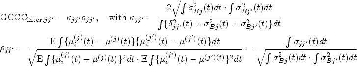
Given a notable overall agreement among the methods, possibly based on the CI of ${\mathrm{GCCC}}_{\mathrm{inter}}$ not containing zero, one may be interested in further investigating which specific pair of methods exhibits significant agreement. This amounts to testing the hypothesis: $H_0:{\mathrm{GCCC}}_{\mathrm{inter},j{j}^{\prime }}=0$ versus $H_a:{\mathrm{GCCC}}_{\mathrm{inter},j{j}^{\prime }}\ne 0$ , where ${\mathrm{GCCC}}_{\mathrm{inter},j{j}^{\prime }}$ denotes the pairwise global inter-CCC between methods $j$ and $j^{\prime }$ . Noting that the pairwise global inter-CCC can be written as

$$\begin{array}{rl}& {\mathrm{GCCC}}_{\mathrm{inter},j{j}^{\prime }}={\kappa }_{j{j}^{\prime }}{\rho }_{j{j}^{\prime }},\text{with}{\kappa }_{j{j}^{\prime }}=\frac{2\sqrt{\int {\sigma }_{Bj}^2(t)dt\cdot \int {\sigma }_{B{j}^{\prime }}^2(t)dt}}{\int \{{\delta }_{j{j}^{\prime }}^2(t)+{\sigma }_{Bj}^2(t)+{\sigma }_{B{j}^{\prime }}^2(t)\}dt}\\ & {\rho }_{j{j}^{\prime }}=\frac{\text{E}\int \{{\mu }_i^{(j)}(t)-{\mu }^{(j)}(t)\}\{{\mu }_i^{(j^{\prime })}(t)-{\mu }^{(j^{\prime })}(t)\}dt}{\sqrt{\text{E}\int \{{\mu }_i^{(j)}(t)-{\mu }^{(j)}(t){\}}^{2}dt\cdot \text{E}\int \{{\mu }_i^{(j^{\prime })}(t)-{\mu }^{(j^{\prime })(t)}{\}}^{2}dt}}=\frac{\int {\sigma }_{j{j}^{\prime }}(t)dt}{\sqrt{\int {\sigma }_{Bj}^2(t)dt\cdot \int {\sigma }_{B{j}^{\prime }}^2(t)dt}}\end{array}$$

that is, the functional correlation coefficient ⁹ ${\rho }_{j{j}^{\prime }}$ scaled by ${\kappa }_{j{j}^{\prime }}$ , one can conduct a permutation test, similar in spirit to that for the correlation, to test this hypothesis. ²² However, performing a permutation test using ${\widehat{\mathrm{GCCC}}}_{\mathrm{inter},j{j}^{\prime }}$ may result in an inflated Type I error rate as permutation and sampling distributions converge to different distributions. ²³ One remedy is to perform the test on the studentized statistic ²² ${\hat{S}}_{j{j}^{\prime }}=\sqrt{n}{\widehat{\mathrm{GCCC}}}_{\mathrm{inter},j{j}^{\prime }}/{\hat{\tau }}_{j{j}^{\prime }}$ , where ${\hat{\tau }}_{j{j}^{\prime }}=\int \{{\hat{\sigma }}_{Bj}^2(t)+{\hat{\sigma }}_{B{j}^{\prime }}^2(t)+2{\hat{\sigma }}_{j{j}^{\prime }}^2(t)\}dt/\{\int {\hat{\sigma }}_{Bj}^2(t)dt\cdot \int {\hat{\sigma }}_{B{j}^{\prime }}^2(t)dt\}$ is the estimator of ${\tau }_{j{j}^{\prime }}={\mu }_{22}^{(j{j}^{\prime })}/({\mu }_{20}^{(j{j}^{\prime })}{\mu }_{02}^{(j{j}^{\prime })})$ with ${\mu }_{rs}^{(j{j}^{\prime })}=\text{E}\int \{{\mu }_i^{(j)}(t)-{\mu }^{(j)}(t){\}}^r\{{\mu }_i^{(j^{\prime })}(t)-{\mu }^{(j^{\prime })}(t){\}}^{s}dt$ , assuming $Z_i^{(j)}(t)\sim N(0,{\sigma }_{Bj}^2(t))$ and $Z_i^{(j^{\prime })}(t)\sim N(0,{\sigma }_{B{j}^{\prime }}^2(t))$ . To summarize, permute the data from method $j^{\prime }$ at the subject level, compute the studentized statistic, repeat the permutation multiple times (e.g. 10,000), and obtain the $p$ -value as the proportion of permutations with an absolute value of the statistic at least as large as the observed one. One can compare the $p$ -value to the significance level adjusted for multiple pairwise comparisons.

3. Simulations

In this section, we conduct simulation studies to examine the finite-sample performance of the proposed procedure for estimating the ICC and CCC indices for functional data.

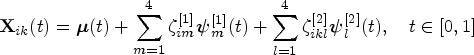
We generate functional data ${\mathbf{X}}_{ik}(t)=(X_{ik}^{(1)}(t),\dots ,X_{ik}^{(J)}(t){)}^{\mathrm{\top }}$ according to the following multivariate multilevel model whose level 1 and 2 functions are expressed using respective multivariate multilevel KL expansion with four components for each level:

$${\mathbf{X}}_{ik}(t)=\mathit{\mu }(t)+\sum _{m=1}^4{\zeta }_{im}^{[1]}{\mathit{\psi }}_m^{[1]}(t)+\sum _{l=1}^4{\zeta }_{ikl}^{[2]}{\mathit{\psi }}_l^{[2]}(t),t\in [0,1]$$

for $i=1,\dots ,n$ and $k=1,\dots ,K$ , where the domain of functional data is a unit interval $\mathcal{T}=[0,1]$ , $\mathit{\mu }(t)=({\mu }^{(1)}(t),\dots ,{\mu }^{(J)}(t){)}^{\mathrm{\top }}$ , ${\mathit{\psi }}_m^{[1]}(t)=({\psi }_m^{[1](1)}(t),\dots ,{\psi }_m^{[1](J)}(t){)}^{\mathrm{\top }}$ , and ${\mathit{\psi }}_l^{[2]}(t)=({\psi }_l^{[2](1)}(t),\dots ,{\psi }_l^{[2](J)}(t){)}^{\mathrm{\top }}$ .

In the first setting, we consider functional data produced by two methods ( $J=2$ ). The level 1 multivariate eigenfunctions are set as ${\psi }_{2v-1}^{[1](j)}(t)=(1.6-0.4j{)}^{0.5}\sin \{2(jv-j+1)\pi t\}$ , ${\psi }_{2v}^{[1](j)}(t)=(1.6-0.4j{)}^{0.5}\cos \{2(jv-j+1)\pi t\}$ for $j=1,2$ and $v=1,2$ . The level 2 multivariate eigenfunctions are set to ${\psi }_{2u-1}^{[2](j)}(t)=(0.4+0.4j{)}^{0.5}\sin \{2(u+2j)\pi t\}$ and ${\psi }_{2u}^{[2](j)}(t)=(0.4+0.4j{)}^{0.5}\cos \{2(u+2j)\pi t\}$ for $u=1,2$ and $j=1,2$ . Two different specifications of the multivariate mean functions are considered: $\mathit{\mu }(t)=(0.5,1{)}^{\mathrm{\top }}$ and $\mathit{\mu }(t)=(0.5t,-0.5t+0.5{)}^{\mathrm{\top }}$ . Here the former mean function is constant over $t$ , while the latter is a linear function of $t$ . In the second setting, functional data are produced by three methods ( $J=3$ ). The level 1 multivariate eigenfunctions are set as ${\psi }_{2v-1}^{[1](j)}(t)=(0.33j{)}^{0.5}\sin \{2(jv-j+1)\pi t\}$ , ${\psi }_{2v}^{[1](j)}(t)=(0.33j{)}^{0.5}\cos \{2(jv-j+1)\pi t\}$ for $j=1,2,3$ and $v=1,2$ . The level 2 multivariate eigenfunctions are set to ${\psi }_{2u-1}^{[2](j)}(t)=(1.33-0.33j{)}^{0.5}\sin \{2(u+2j)\pi t\}$ and ${\psi }_{2u}^{[2](j)}(t)=(1.33-0.33j{)}^{0.5}\cos \{2(u+2j)\pi t\}$ for $u=1,2$ and $j=1,2,3$ . Two different specifications of the multivariate mean functions that we consider are $\mathit{\mu }(t)=(0.5,0.8,1.1{)}^{\mathrm{\top }}$ and $\mathit{\mu }(t)=(0.5t,0.8t,-0.8t+0.8{)}^{\mathrm{\top }}$ .

In both settings, the scores ${\zeta }_{im}^{[1]}$ and ${\zeta }_{ikl}^{[2]}$ are independently generated from $N(0,{\lambda }_m^{[1]})$ and $N(0,{\lambda }_l^{[2]})$ , respectively, where ${\lambda }_m^{[1]}={0.5}^{m-1}$ $(m=1,\dots ,4)$ , and ${\lambda }_l^{[2]}={0.5}^{l-1}$ $(l=1,\dots ,4)$ . Sample sizes are set as $n=100$ and $n=300$ , and the number of replicates produced by each method on each subject is set to $K=3$ . All functional data are generated on a grid of $T$ equidistant time points $\{(t-1)/(T-1);t=1,\dots ,T\}$ , with $T=50$ and $100$ . In sum, we consider 16 scenarios $=2(J=2\text{or}J=3)\times 2$ (two different specifications of $\mu )\times 2(n=100\text{or}300)\times 2(T=50\text{or}100)$ .

The accuracy of the CCC and ICC estimates computed using the procedure described in Section 2.4 is measured by “average bias” $T^{-1}\sum _{h=1}^{\mathrm{T}}\{\widehat{\text{CCC}}(t_h)-\text{CCC}(t_h)\}$ for the time-dependent indices and “bias” $\widehat{\text{GCCC}}-\text{GCCC}$ for the global indices. The biases are calculated and averaged across 500 simulated data sets. We also report the coverage rates of pointwise 95% bootstrap confidence bands (averaged across time points) and 95% bootstrap CIs on 500 simulated data sets. Here, the intervals are constructed using $B=200$ bootstrap resamples at the subject level. Note that during estimation and inference, the numbers of level 1 and 2 components to retain ( $M_{*}^{[1]}$ and $M_{*}^{[2]}$ ) are chosen to preserve 95% of the total variability in each simulated data set.

Tables 1 and 2 present the simulation results for the two settings with $J=2$ and $J=3$ methods, respectively. We immediately see that, in all configurations, the biases of all estimated indices are small and approach 0 as the sample size ( $n$ ) and number of time points ( $T$ ) increase, demonstrating the adequate accuracy and consistency of our estimation procedure. Note that both time-dependent and global inter-CCC indices ( ${\mathrm{CCC}}_{\mathrm{inter}}(t)$ and ${\mathrm{GCCC}}_{\mathrm{inter}}$ ) exhibit slightly higher bias (but still reasonably low) compared to other indices. This is mainly because the inter-CCC indices are based on the squared expected difference between the true readings that are not directly observed, further complicating their estimation task. However, we do see that their biases quickly approach 0 as the sample size and number of time points increase. The coverage rates of the pointwise 95% bootstrap confidence bands for time-dependent indices and the 95% bootstrap CIs for global indices are all close to 0.95. Again, the coverage rate of ${\mathrm{GCCC}}_{\mathrm{inter}}$ is slightly lower (but still over 0.92) than those of other indices when $n=100$ and $T=50$ , but it quickly approaches the nominal level as $n$ and $T$ increase. In summary, our simulation studies demonstrate the satisfactory finite-sample performance of the proposed estimation and inference schemes.

Table 1.

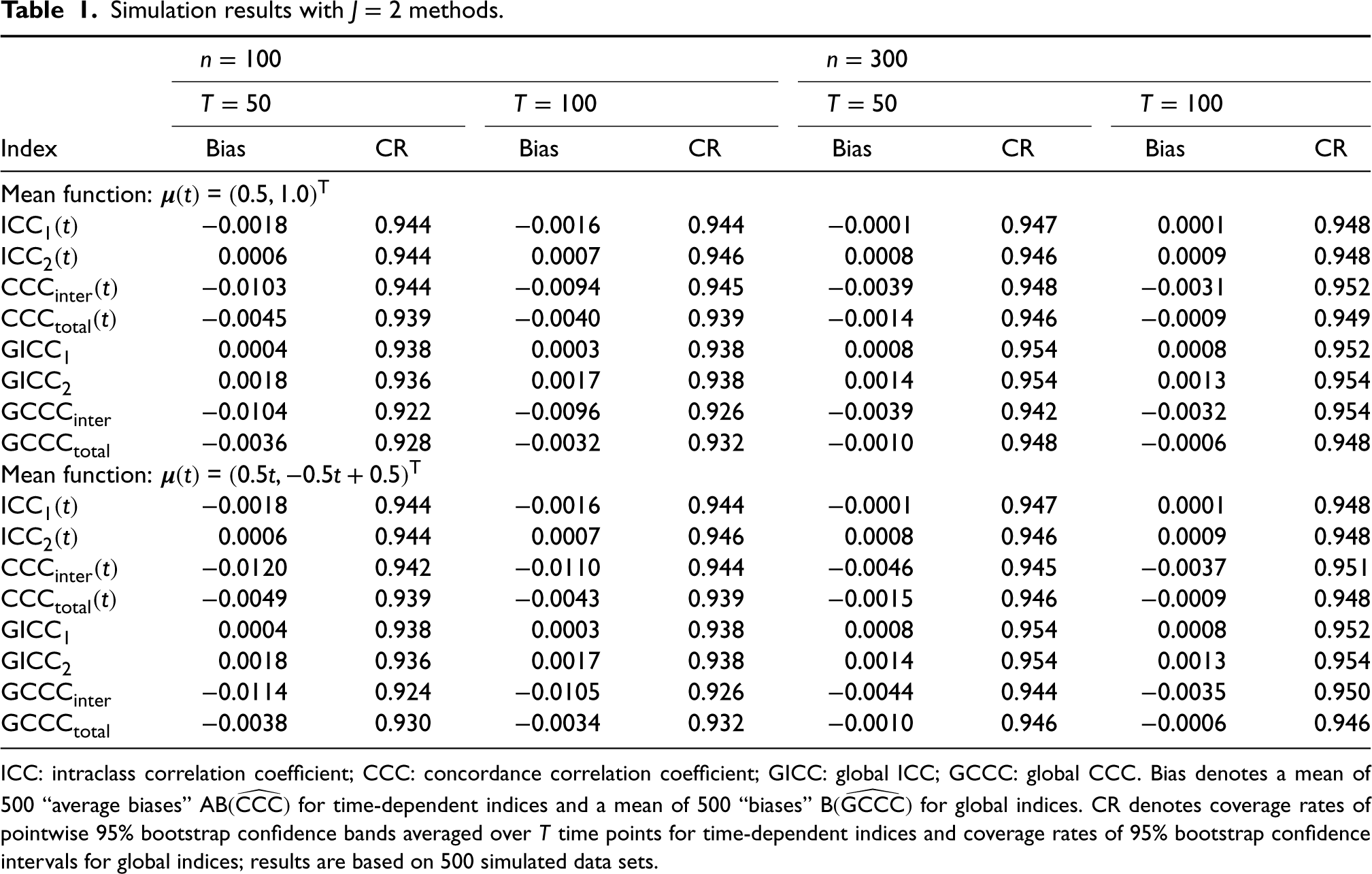
Simulation results with $J=2$ methods.

	$n=100$				$n=300$
	$T=50$		$T=100$		$T=50$		$T=100$
Index	Bias	CR	Bias	CR	Bias	CR	Bias	CR
Mean function: $\mathit{\mu }(t)$ = $(0.5,1.0{)}^{\mathrm{T}}$
${\mathrm{ICC}}_1(t)$	−0.0018	0.944	−0.0016	0.944	−0.0001	0.947	0.0001	0.948
${\mathrm{ICC}}_2(t)$	0.0006	0.944	0.0007	0.946	0.0008	0.946	0.0009	0.948
${\mathrm{CCC}}_{\mathrm{inter}}(t)$	−0.0103	0.944	−0.0094	0.945	−0.0039	0.948	−0.0031	0.952
${\mathrm{CCC}}_{\mathrm{total}}(t)$	−0.0045	0.939	−0.0040	0.939	−0.0014	0.946	−0.0009	0.949
${\mathrm{GICC}}_1$	0.0004	0.938	0.0003	0.938	0.0008	0.954	0.0008	0.952
${\mathrm{GICC}}_2$	0.0018	0.936	0.0017	0.938	0.0014	0.954	0.0013	0.954
${\mathrm{GCCC}}_{\mathrm{inter}}$	−0.0104	0.922	−0.0096	0.926	−0.0039	0.942	−0.0032	0.954
${\mathrm{GCCC}}_{\mathrm{total}}$	−0.0036	0.928	−0.0032	0.932	−0.0010	0.948	−0.0006	0.948
Mean function: $\mathit{\mu }(t)$ = $(0.5t,-0.5t+0.5{)}^{\mathrm{T}}$
${\mathrm{ICC}}_1(t)$	−0.0018	0.944	−0.0016	0.944	−0.0001	0.947	0.0001	0.948
${\mathrm{ICC}}_2(t)$	0.0006	0.944	0.0007	0.946	0.0008	0.946	0.0009	0.948
${\mathrm{CCC}}_{\mathrm{inter}}(t)$	−0.0120	0.942	−0.0110	0.944	−0.0046	0.945	−0.0037	0.951
${\mathrm{CCC}}_{\mathrm{total}}(t)$	−0.0049	0.939	−0.0043	0.939	−0.0015	0.946	−0.0009	0.948
${\mathrm{GICC}}_1$	0.0004	0.938	0.0003	0.938	0.0008	0.954	0.0008	0.952
${\mathrm{GICC}}_2$	0.0018	0.936	0.0017	0.938	0.0014	0.954	0.0013	0.954
${\mathrm{GCCC}}_{\mathrm{inter}}$	−0.0114	0.924	−0.0105	0.926	−0.0044	0.944	−0.0035	0.950
${\mathrm{GCCC}}_{\mathrm{total}}$	−0.0038	0.930	−0.0034	0.932	−0.0010	0.946	−0.0006	0.946

ICC: intraclass correlation coefficient; CCC: concordance correlation coefficient; GICC: global ICC; GCCC: global CCC. Bias denotes a mean of 500 “average biases” $\text{AB}(\widehat{\text{CCC}})$ for time-dependent indices and a mean of 500 “biases” $\text{B}(\widehat{\text{GCCC}})$ for global indices. CR denotes coverage rates of pointwise 95% bootstrap confidence bands averaged over $T$ time points for time-dependent indices and coverage rates of 95% bootstrap confidence intervals for global indices; results are based on 500 simulated data sets.

Table 2.

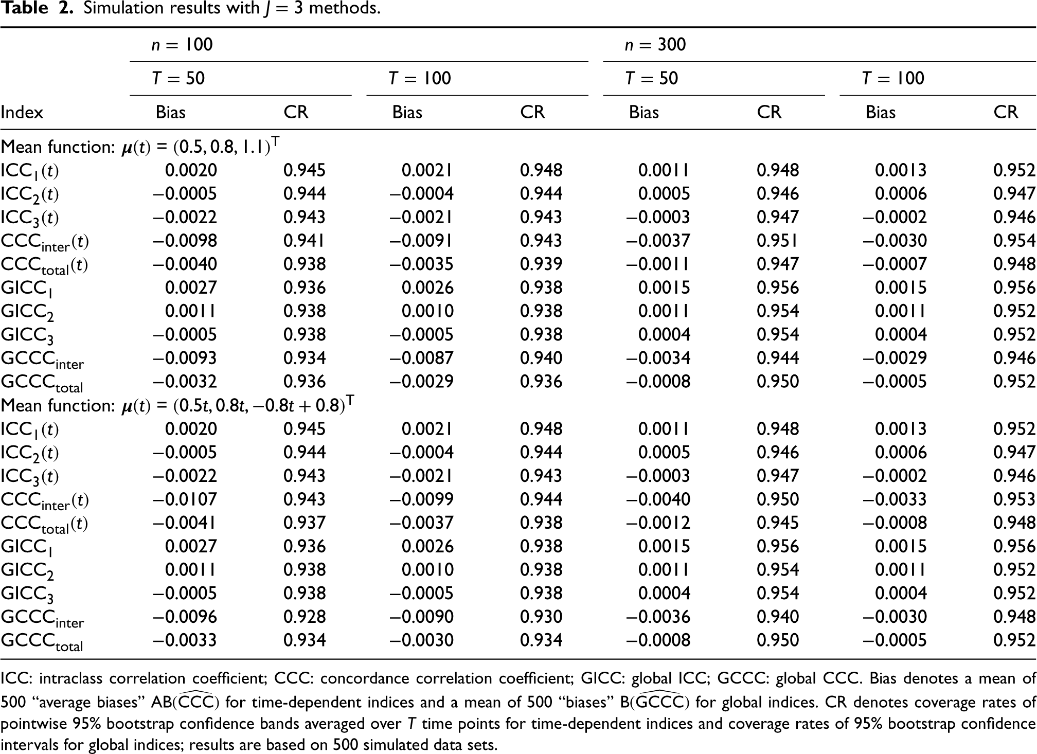
Simulation results with $J=3$ methods.

	$n=100$				$n=300$
	$T=50$		$T=100$		$T=50$		$T=100$
Index	Bias	CR	Bias	CR	Bias	CR	Bias	CR
Mean function: $\mathit{\mu }(t)$ = $(0.5,0.8,1.1{)}^{\mathrm{T}}$
${\mathrm{ICC}}_1(t)$	0.0020	0.945	0.0021	0.948	0.0011	0.948	0.0013	0.952
${\mathrm{ICC}}_2(t)$	−0.0005	0.944	−0.0004	0.944	0.0005	0.946	0.0006	0.947
${\mathrm{ICC}}_3(t)$	−0.0022	0.943	−0.0021	0.943	−0.0003	0.947	−0.0002	0.946
${\mathrm{CCC}}_{\mathrm{inter}}(t)$	−0.0098	0.941	−0.0091	0.943	−0.0037	0.951	−0.0030	0.954
${\mathrm{CCC}}_{\mathrm{total}}(t)$	−0.0040	0.938	−0.0035	0.939	−0.0011	0.947	−0.0007	0.948
${\mathrm{GICC}}_1$	0.0027	0.936	0.0026	0.938	0.0015	0.956	0.0015	0.956
${\mathrm{GICC}}_2$	0.0011	0.938	0.0010	0.938	0.0011	0.954	0.0011	0.952
${\mathrm{GICC}}_3$	−0.0005	0.938	−0.0005	0.938	0.0004	0.954	0.0004	0.952
${\mathrm{GCCC}}_{\mathrm{inter}}$	−0.0093	0.934	−0.0087	0.940	−0.0034	0.944	−0.0029	0.946
${\mathrm{GCCC}}_{\mathrm{total}}$	−0.0032	0.936	−0.0029	0.936	−0.0008	0.950	−0.0005	0.952
Mean function: $\mathit{\mu }(t)$ = $(0.5t,0.8t,-0.8t+0.8{)}^{\mathrm{T}}$
${\mathrm{ICC}}_1(t)$	0.0020	0.945	0.0021	0.948	0.0011	0.948	0.0013	0.952
${\mathrm{ICC}}_2(t)$	−0.0005	0.944	−0.0004	0.944	0.0005	0.946	0.0006	0.947
${\mathrm{ICC}}_3(t)$	−0.0022	0.943	−0.0021	0.943	−0.0003	0.947	−0.0002	0.946
${\mathrm{CCC}}_{\mathrm{inter}}(t)$	−0.0107	0.943	−0.0099	0.944	−0.0040	0.950	−0.0033	0.953
${\mathrm{CCC}}_{\mathrm{total}}(t)$	−0.0041	0.937	−0.0037	0.938	−0.0012	0.945	−0.0008	0.948
${\mathrm{GICC}}_1$	0.0027	0.936	0.0026	0.938	0.0015	0.956	0.0015	0.956
${\mathrm{GICC}}_2$	0.0011	0.938	0.0010	0.938	0.0011	0.954	0.0011	0.952
${\mathrm{GICC}}_3$	−0.0005	0.938	−0.0005	0.938	0.0004	0.954	0.0004	0.952
${\mathrm{GCCC}}_{\mathrm{inter}}$	−0.0096	0.928	−0.0090	0.930	−0.0036	0.940	−0.0030	0.948
${\mathrm{GCCC}}_{\mathrm{total}}$	−0.0033	0.934	−0.0030	0.934	−0.0008	0.950	−0.0005	0.952

ICC: intraclass correlation coefficient; CCC: concordance correlation coefficient; GICC: global ICC; GCCC: global CCC. Bias denotes a mean of 500 “average biases” $\text{AB}(\widehat{\text{CCC}})$ for time-dependent indices and a mean of 500 “biases” $\text{B}(\widehat{\text{GCCC}})$ for global indices. CR denotes coverage rates of pointwise 95% bootstrap confidence bands averaged over $T$ time points for time-dependent indices and coverage rates of 95% bootstrap confidence intervals for global indices; results are based on 500 simulated data sets.

Furthermore, we perform additional simulation studies with error-prone functional data; that is, $Y_{ik}^{(j)}(t)=X_{ik}^{(j)}(t)+{ϵ}_{ik}^{(j)}(t)$ , where true signals $X_{ik}^{(j)}$ are generated under the aforementioned data generation scenarios, and ${ϵ}_{ik}^{(j)}(t)$ is an independent residual noise iid $N(0,{0.1}^2)$ . The errors are handled by representing the functions using B-splines with 25 basis functions and controlling their smoothness by introducing a roughness penalty term (integral of the square of the second derivative). The same evaluation scheme as above is applied. The simulation results are presented in Tables S1 and S2 of the Supplemental Materials, and they demonstrate the satisfactory finite-sample performance of the proposed estimation and inference schemes with error-prone functional data.

4. Application to Emory renal study

In this section, we apply the proposed methodology to the Emory renal study described in Section 1. The study collected renogram data from $n=100$ kidneys of patients who were referred to the Emory University Hospital with suspected kidney obstruction from 1 May 1994 to 4 July 2015. For each kidney, renogram curves, which consist of MAG3 photon counts detected at 100 time points (every 12–15 s) over a period of 1428 s on the ROI, were produced by $J=2$ different methods: the “whole-kidney ROI method” ( $j=1$ ) and “cortical-kidney ROI method” ( $j=2$ ). Each method was repeated two times $(K=2)$ by the attending radiologist, who manually specified the ROI on the kidney on each occasion. In sum, four renogram curves (two curves produced by the whole-kidney ROI method plus two curves produced by the cortical-kidney ROI method) were available for each kidney, and accordingly the collection of observed renogram curve data can be expressed using mathematical notation as $\{X_{ik}^{(j)}(t_h):i=1,\dots ,100;j=1,2;k=1,2;h=1,\dots ,100\}$ with each $t_h\in \mathcal{T}=[0,1428]$ .

One of the main goals of the study is to evaluate the reproducibility and reliability of MAG3 renography, which is a state-of-the-art medical device widely used to non-invasively detect kidney obstruction. Specifically, the researchers aim to achieve this goal by answering the following two scientific questions: (i) do twice-repeated renogram curves produced on the same kidney by each method agree (intra-method agreement); and (ii) do renogram curves produced by the two methods agree (inter-method agreement). To address these two questions, the proposed indices are estimated based on the procedure introduced in Section 2.4. Note that the eigenanalyses of the smoothed covariance function estimates are performed to account for residual noise in the renogram curves. We also note that the numbers of level 1 and 2 components to retain ( $M_{*}^{[1]}$ and $M_{*}^{[2]}$ ) are chosen to preserve 95% of the total variability in the data, and the pointwise 95% bootstrap confidence bands and 95% bootstrap CIs are constructed based on $B=200$ bootstrap resamples at the kidney level. Web Figures S1 and S2 of the Supplemental Materials, respectively, present the estimated mean functions, ${\hat{\mu }}^{(1)}(t)$ and ${\hat{\mu }}^{(2)}(t)$ , and the estimated variance components, ${\hat{\sigma }}_{B1}^2(t)$ , ${\hat{\sigma }}_{B2}^2(t)$ , ${\hat{\sigma }}_{W1}^2(t)$ , ${\hat{\sigma }}_{W2}^2(t)$ , and ${\hat{\sigma }}_{12}(t)$ .

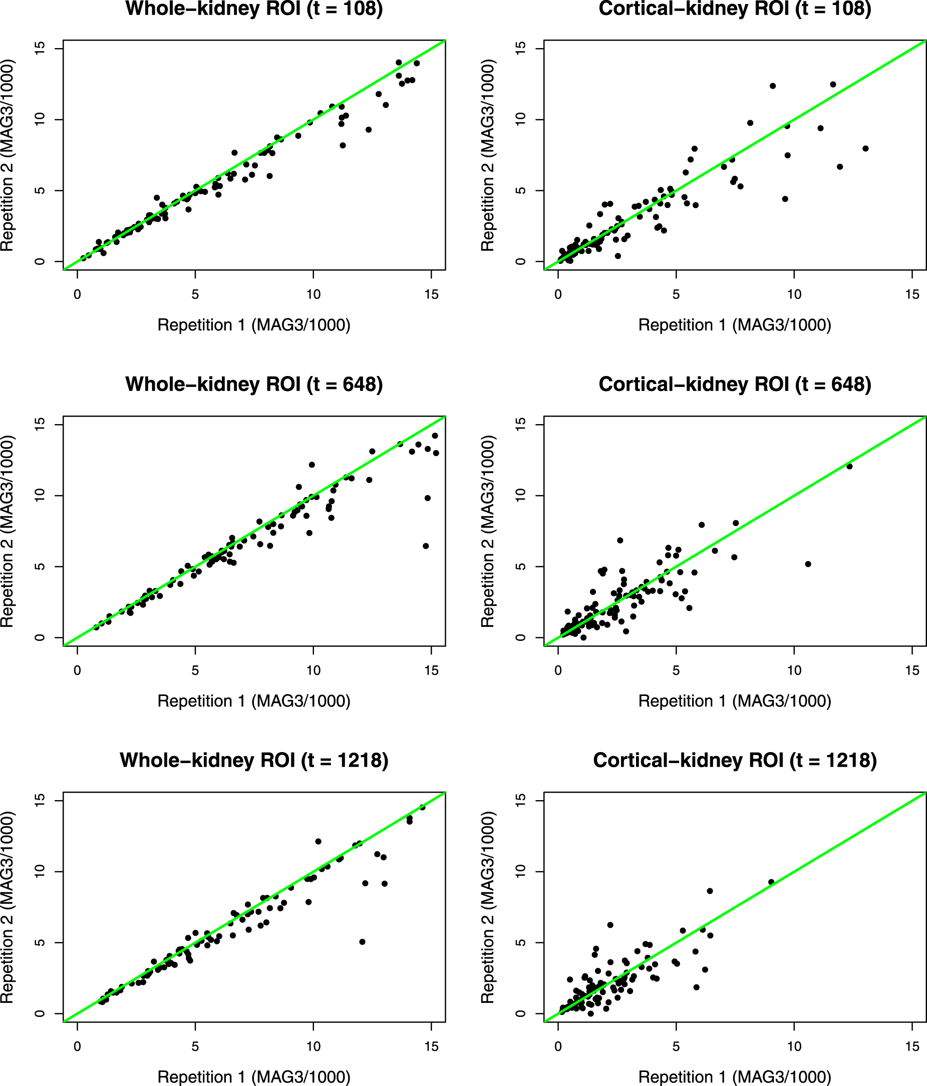
Regarding the first question, we first examine the scatterplots whose horizontal and vertical axes are MAG3 photon counts of the first and second repetitions, respectively, produced by each method at scan times $t=108$ , $648$ , and 1218; see Figure 2. At all time points, we see that the points are more tightly clustered around the 45-degree line for the whole-kidney ROI method, suggesting its superior intra-method agreement compared to the cortical-kidney ROI method.

Figure 2.

Scatterplots whose horizontal and vertical axes respectively represent the MAG3 photon counts (divided by 1000) of the first and second repetitions, respectively, produced by each of the methods (left panel: whole-kidney ROI method; right panel: cortical-kidney ROI method at scan times $t=108$ (top panel), $t=648$ (middle panel), and $t=1218$ (bottom panel). MAG3: mercaptoacetyltriglycine; ROI: region of interest.

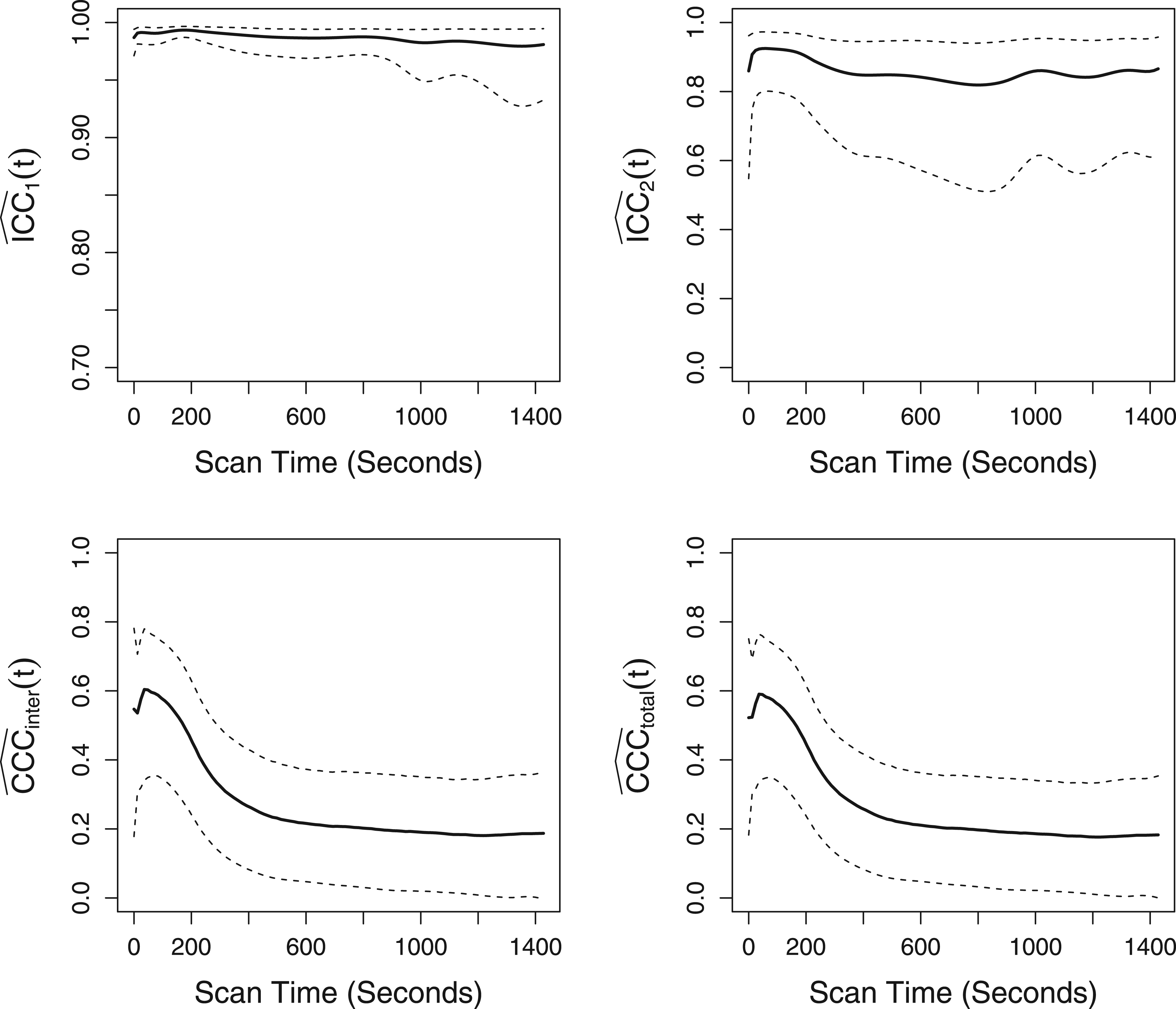
To formally assess intra-method agreement, the proposed ICC indices, ${\mathrm{ICC}}_1(t)$ and ${\mathrm{ICC}}_2(t)$ , are estimated and displayed in the top panel of Figure 3. The estimated time-dependent ICC for the whole-kidney ROI method, ${\widehat{\mathrm{ICC}}}_1(t)$ , hovers above 0.95 over the entire scan period. Accordingly, a high global ICC ( ${\widehat{\mathrm{GICC}}}_1$ ) value of 0.986 (95% CI: $[0.967,0.994]$ ) is obtained. This high intra-method agreement suggests that the whole-kidney ROI method is robust to and reproducible across multiple ROI specification tasks performed by a practicing radiologist. For the cortical-kidney ROI method, ${\widehat{\mathrm{ICC}}}_2(t)$ hovers over 0.8 over the entire scan period, and the corresponding global ICC value ${\widehat{\mathrm{GICC}}}_2=0.859$ (95% CI: $[0.635,0.950]$ ). This suggests that the cortical-kidney ROI method has moderate intra-method agreement and is not as reproducible as the whole-kidney ROI method over repeated ROI specification tasks by a practicing radiologist.

Figure 3.

The top panel presents the estimated time-dependent ICC indices (bold line) for the whole-kidney ROI method (left) and the cortical-kidney ROI method (right), along with their pointwise 95% bootstrap confidence bands (dashed line). The bottom panel presents the estimated time-dependent inter-CCC index (left; bold line) and total-CCC index (right; bold line) between the whole-kidney ROI and cortical kidney ROI methods, along with their pointwise 95% bootstrap confidence bands (dashed line). Note the differing scale on the vertical axes for the top left panel. ICC: intraclass correlation coefficient; ROI: region of interest.

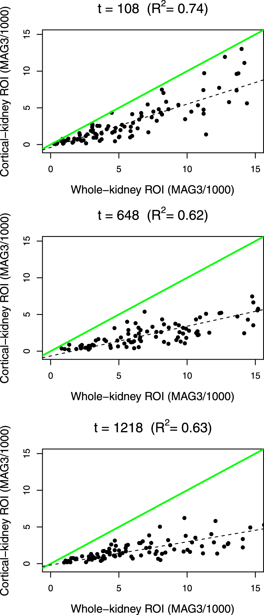
Regarding the second question, we first examine the scatterplot of MAG3 counts between the first replications of the whole-kidney ROI (horizontal axis) and cortical-kidney ROI (vertical axis) methods at scan times $t=108$ , $648$ , and $1218$ ; see Figure 4. At each of the time points, we see that the paired measurements are positively correlated with an R-squared value >0.6, but the deviation of the least-squares line (dashed line) from the 45-degree line (solid line) increases as the photon count increases, suggesting a location and scale shift of one method from the other.

Figure 4.

Scatterplots of MAG3 photon counts (divided by 1000) between the first replications of the whole-kidney ROI method (horizontal axis) and the cortical-kidney ROI method (vertical axis) at time points $t=108$ (top panel), $t=648$ (middle panel), and $t=1218$ (bottom panel). The green (gray in print) solid line denotes the 45-degree line. The black dashed line represents the least-squares line. $R^2$ denotes the R-squared value between the measurements from the two methods at each time point. MAG3: mercaptoacetyltriglycine; ROI: region of interest.

To formally assess inter-method agreement between the whole-kidney ROI and cortical-kidney ROI methods, we estimate ${\widehat{\mathrm{CCC}}}_{\mathrm{inter}}(t)$ and obtain its pointwise 95% bootstrap confidence band. In the bottom right panel of Figure 3, we see that the degree of inter-method agreement between the two methods hovers below 0.3 during most of the scan period except the initial phase of 0–250 s. Accordingly, the global CCC is low ( ${\widehat{\mathrm{GCCC}}}_{\mathrm{inter}}=0.247$ ; 95% CI: $[0.085,0.395]$ ). To investigate the source of disagreement between the two methods, we estimate ${\rho }_{12}(t)$ , $v_{12}(t)$ and $u_{12}(t)$ , which, respectively, measure the degrees of precision, scale shift, and location shift; see Figure S3 of the Supplemental Materials. The ${\hat{\rho }}_{12}(t)$ trajectory (top panel) starts around 0.8, gradually decreases to approximately 0.5 until $t=400$ , and then stabilizes afterward, indicating a moderate precision (correlation) between the true readings of the two methods. The major source of disagreement is the shift in scale and location. Specifically, the ${\hat{v}}_{12}(t)$ trajectory (middle panel) starts around 2 and then gradually increases up to 2.8, indicating that the scale of the whole-kidney ROI method is larger than that of the cortical-kidney ROI method. The ${\hat{u}}_{12}(t)$ trajectory (bottom panel) hovers between 1 and 1.5 during most of the scan period after the initial phase of 0–250 s and shows that the measurements of the whole-kidney ROI method are shifted right relative to those of the cortical-kidney ROI method. These results suggest that the agreement between the two methods is not acceptable, and one method cannot completely replace the other. The estimated total agreement indices, ${\widehat{\mathrm{CCC}}}_{\mathrm{total}}(t)$ (see bottom right panel of Figure 3) and ${\widehat{\mathrm{GCCC}}}_{\mathrm{total}}=0.241$ (95% CI: $[0.086,0.384]$ ), which contain both intra- and inter-method agreement, show similar trends, though they are slightly lower than the inter-agreement counterparts.

In conclusion, the moderate to high intra-method agreement suggests that both whole-kidney ROI and cortical-kidney ROI methods generate renogram curves that are quite reproducible across multiple ROI specification tasks manually performed by a practicing radiologist. These results lend support to establishing both methods as a robust basis for diagnostic evaluation of kidney obstruction. Between the two methods, we found that the whole-kidney ROI method produces more consistent and thus more reliable renogram curves across multiple ROI specifications compared to the cortical-kidney ROI method. This is possibly because the renogram curves produced by the cortical-kidney ROI method can be relatively more noisy on the region overlying the liver (a very vascular organ), where the MAG3 in the blood may be superimposed on the cortical curve. ²⁴ Thus, given the high/moderate but imperfect intra-method agreement, a practicing radiologist may produce and study multiple renogram curves from each method (especially for the cortical-kidney ROI method with relatively low intra-method agreement) to safeguard against possible inconsistency in its readings across multiple attempts. Furthermore, the low inter-method agreement between the two methods (i.e. one method cannot completely replace the other) indicates that both renogram curves should be studied and interpreted by a practicing radiologist to diagnose kidney obstruction. In fact, this conclusion aligns with that of previous research,^14,24 which states that each method captures unique physiological mechanisms linked to kidney obstruction, and the best practice to capture all relevant physiological mechanisms and maximize diagnostic accuracy is to simultaneously examine pharmacokinetic features of renogram curves from both methods (e.g. whole-kidney ROI postvoid/max count ratio and cortical-kidney ROI time-to-maximum).

5. Discussion

In this paper, we introduced a set of time-dependent ICC and CCC indices that quantify the degrees of intra-method, inter-method, and total agreement varying smoothly over time and global counterparts that summarize such agreement over time using a single measure. We take a model-based approach for defining and estimating the proposed indices. Specifically, the functional data measurements are modeled using a multivariate multilevel functional mixed effects model, which enables us to express the indices as variance components and smoothly estimate them by FPCA. An extensive simulation study was performed to demonstrate that our estimation and inference procedures produce consistent estimators and CIs with adequate coverage, respectively. In application to renal study data, the proposed unscaled indices were computed to obtain new and interesting insights into the reliability and reproducibility of modern diuresis renography for kidney obstruction diagnosis. We note that the proposed methodology is generally applicable and transferable to quantify the reliability and reproducibility of any modern medical device producing various functional data measurements including images and tensors (two- or three-dimensional functional data).

In our work, we expressed the random effect functions and variance components of the multivariate multilevel functional mixed model (2) in finite-dimensional forms using principal components (eigenfunctions). Using principal components as data-driven basis functions has several advantages compared to using pre-specified basis functions (e.g. B-splines, Fourier basis, etc.). Firstly, principal components represent the directions of the data that capture most of the between- and within-subject variabilities, enabling us to derive the indices that can assess the agreement of functional data while focusing on their most important features. Secondly, the principal component scores which are used as lower-dimensional representations of the random effect functions—see (3)—are estimated simultaneously using all data, facilitating borrowing of information across different observation units and coherent characterization of uncertainty.

One limitation of the FPCA approach is that if measurements generated by different methods differ considerably in domain, range, or variation, there is a possibility that FPCA components are dominated by data from one or few methods with larger variances. However, the main goal of our study (as in other agreement studies) is to quantify the degree of reproducibility among methods/raters that generate clinical measurements of the same unit representing a certain common biological or disease mechanism, in which case clinical measurements from different methods do not usually differ in domain, range, or variation to a degree that one or few methods completely dominate the FPCA components. In the past FPCA literature, multivariate FPCA has been successfully applied to identify any major co-varying patterns of multivariate functional data without scaling when their measurements are in the same unit and do not grossly differ in range, domain, or variation.^15,13

In some rare cases, researchers might have to assess agreement among methods that generate functional clinical measurements that grossly differ in domain, range, or variation. One simple remedy is to scale the data so that each of the multivariate functions has integrated variance equal to 1. ¹³ This approach, however, prevents our indices from identifying and incorporating disagreement due to scale shift; they can only identify disagreement due to lack of precision and location shift. Another possible approach is to model the clinical measurements based on recently introduced “structured FPCA” ²⁵ as following

$$Y_{ijk}(t)=\mu (t)+{\eta }_j(t)+U_i(t)+V_{ij}(t)+W_{ijk}(t)+{ϵ}_{ijkt}$$

where $Y_{ijk}(t)$ is denotes the $k$ th repeated functional clinical measurement from method $j$ for subject $i$ , $\mu (t)$ is a deterministic overall mean function, ${\eta }_j(t)$ is a deterministic method-specific mean function, $U_i(t)$ is a subject-specific random function with covariance operator $K_U(s,t)=\text{Cov}\{U_i(s),U_i(t)\}$ , $V_{ij}(t)$ is a subject-method-specific random function with covariance $K_V(s,t)=\text{Cov}\{V_{ij}(s),V_{ij}(t)\}$ , $W_{ijk}(t)$ is a random function representing the remaining variation in $X_{ijk}(t)$ not explained by the first two random functions and has covariance $K_W(s,t)=\text{Cov}\{W_{ijk}(s),W_{ijk}(t)\}$ , and ${ϵ}_{ijkt}\stackrel{\text{iid}}{\sim }(0,{\sigma }^2)$ is a white noise. To ensure identifiability, the random processes $U_i(t)$ , $V_{ij}(t)$ and $W_{ijk}(t)$ are assumed to have mean-zero and be uncorrelated. This approach is free from the problem of one or a few methods with larger variances dominating the FPCA components. However, a major limitation of this approach is that it requires the between-subject variance ${\sigma }_{Bj}^2(t)=\text{Var}\{U_i(t)+V_{ij}(t)\}=K_U(t,t)+K_V(t,t)$ , within-subject variance ${\sigma }_{Wj}^2(t)=\text{Var}\{W_{ijk}(t)\}=K_W(t,t)$ and between-subject covariance ${\sigma }_{j{j}^{\prime }}(t)=\text{Cov}\{U_i(t)+V_{ij}(t),U_i(t)+V_{i{j}^{\prime }}(t)\}=K_U(t,t)$ are shared across all methods and thus severely restricts the applicability of the ICCs and CCCs formulated based upon them. Specifically, under this formulation, the ICC (5) takes on common values across all methods, and the inter-CCC (6) and total-CCC (7) can only capture discrepancies in the means (location shifts). Given these limitations of the current approaches, our future research direction is to develop a model framework under which agreement indices can not only capture discrepancies due to various disagreement types (lack of precision, scale shift, and location shift), but also admit an estimation scheme that is unaffected by extreme differences of multivariate functional measurements in domain, range, or variation.

Supplemental Material

sj-pdf-1-smm-10.1177_09622802231219862 - Supplemental material for Assessing intra- and inter-method agreement of functional data

Supplemental material, sj-pdf-1-smm-10.1177_09622802231219862 for Assessing intra- and inter-method agreement of functional data by Ye Yue, Jeong Hoon Jang and Amita K. Manatunga in Statistical Methods in Medical Research

Supplemental Material

sj-r-2-smm-10.1177_09622802231219862 - Supplemental material for Assessing intra- and inter-method agreement of functional data

Supplemental material, sj-r-2-smm-10.1177_09622802231219862 for Assessing intra- and inter-method agreement of functional data by Ye Yue, Jeong Hoon Jang and Amita K. Manatunga in Statistical Methods in Medical Research

Supplemental Material

sj-r-3-smm-10.1177_09622802231219862 - Supplemental material for Assessing intra- and inter-method agreement of functional data

Supplemental material, sj-r-3-smm-10.1177_09622802231219862 for Assessing intra- and inter-method agreement of functional data by Ye Yue, Jeong Hoon Jang and Amita K. Manatunga in Statistical Methods in Medical Research