
Abstract
Assessing associations between a response of interest and a set of covariates in spatial areal models is the leitmotiv of ecological regression. However, the presence of spatially correlated random effects can mask or even bias estimates of such associations due to confounding effects if they are not carefully handled. Though potentially harmful, confounding issues have often been ignored in practice leading to wrong conclusions about the underlying associations between the response and the covariates. In spatio-temporal areal models, the temporal dimension may emerge as a new source of confounding, and the problem may be even worse. In this work, we propose two approaches to deal with confounding of fixed effects by spatial and temporal random effects, while obtaining good model predictions. In particular, restricted regression and an apparently—though in fact not—equivalent procedure using constraints are proposed within both fully Bayes and empirical Bayes approaches. The methods are compared in terms of fixed-effect estimates and model selection criteria. The techniques are used to assess the association between dowry deaths and certain socio-demographic covariates in the districts of Uttar Pradesh, India.
Introduction
Spatial and spatio-temporal disease mapping techniques have been widely used in epidemiology and public health. Though these analyses are somewhat descriptive, they have undoubted value as they provide information about the geographical pattern of the disease, how this pattern evolves in time, and where regions with extreme risk (high or low) are located. An overall spatio-temporal view of the phenomenon under study is extremely useful for generating hypotheses about factors that may be associated with the disease. Throughout this article and to avoid any misleading conclusion, a risk factor is simply a predictor of one outcome (i.e., cancer, or crimes against women in this article), which can be useful for identifying those areas with high risk requiring special actions or intervention programmes.
When covariates related to the study question are unknown, spatio-temporal areal models are a first step in developing an understanding of the disease or crime under study. Incorporating potential risk factors in a model is usually known as ecological regression, and it confers an inferential perspective on spatio-temporal areal models as it quantifies the relationship between a response and covariates (see, e.g., Martínez-Beneito and Botella-Rocamora (2019)).
Spatio-temporal areal models are practical and valuable tools, but they are not free from inconveniences. Goicoa et al.(2018)Goicoa, Adin, Ugarte, and Hodges highlight some identifiability problems involving the intercept and the spatial and temporal main effects, and involving the main effects and the interaction. To overcome these problems, these authors propose to reparameterize the models or to use constraints, though other approaches exist (see, e.g., Fahrmeir and Lang (2000); Kneib et al.(2019)Kneib, Klein, Lang, and Umlauf for identifiability issues in a class of generalized additive models). Another key issue in spatial and spatio-temporal areal models is potential confounding between the fixed effects and random effects. Spatial confounding occurs when the covariates have a spatial pattern and are collinear with the spatial random effects. Although some authors warn about its effects (see, e.g., Clayton et al.(1993)Clayton, Bernardinelli, and Montomoli; Zadnik and Reich (2006)), it has been and still is often ignored in practice. Though we restrict our attention to models for areal data, the effects of spatial confounding have been studied in other areas such as causal inference (see for example Papadogeorgou et al.(2019)Papadogeorgou, Choirat, and Zigler), or interpolation/prediction (Page et al.(2017)Page, Liu, He, and Sun). Reich et al.(2006)Reich, Hodges, and Zadnik show that adding a conditional autoregressive spatial random effect (CAR) to a fixed effects model can lead to a great change in the posterior mean or a great increase in the posterior variance of the fixed effects, compared to the non-spatial regression model. More precisely, these authors reconsider the Slovenia stomach cancer data, and observe that when the CAR random effect is included in the model, the relationship between stomach cancer and the covariate is diluted. To overcome this problem, they proposed to specify the random effects as orthogonal to the fixed effects. Later, Hodges and Reich (2010) explain why such spatial confounding occurs, and show that adding spatially correlated random effects does not adjust fixed effects for spatially structured missing covariates, as has been generally understood, though they do smooth fitted values.
Following the approach of reparameterizing random effects, Schnell and Bose (2019) also examine the mechanisms of confounding of fixed effects by random effects but they focus on diagnostics to evaluate the effects of confounding rather than on methods to overcome it. Additional work includes Hughes and Haran (2013), Hanks et al.(2015)Hanks, Schliep, Hooten, and Hoeting and Prates et al.(2019)Prates, Assunção, Rodrigues, et al.. Recently, Khan and Calder (2020) observe that restricted regression offers inference similar to models without random effects. Khan and Calder, however, did not discuss model fit or prediction.
The present article deals with spatio-temporal models with covariates and spatial, temporal, and spatio-temporal random effects, pursuing two main goals, namely, correct estimation of linear association between socio-demographic covariates and dowry death (a crime against women very specific to India), and good model predictions. Because we have data and covariates in space and time, confounding may be spatial, temporal or both, and it may mask the association of the outcome with the covariates.
This article proposes different methods to deal with confounding but also with identifiability, as identifying spatial, temporal and spatio-temporal random effects is important for interpretation. On one hand we consider restricted spatial regression (Reich et al.(2006)Reich, Hodges, and Zadnik) and study its application to a spatio-temporal setting. On the other hand, we examine use of constraints to deal with both identifiability and confounding issues. While both methods seem to solve the confounding issue, they lead to notably different results in terms of model fit. Here, we try to disentangle why this happens.
The rest of the article is organized as follows. Section 2 poses the spatial and the spatio-temporal models and briefly revisits identifiability and confounding issues. Section 3 proposes two procedures to alleviate confounding and identify the model: a model reparameterization followed by restricted regression, and the use of orthogonality constraints. In Section 4, both techniques are used to assess the association between dowry death and socio-demographic covariates, and to predict spatio-temporal patterns of risk in Uttar Pradesh, the most populated state in India.
Pitfalls in spatial and spatio-temporal areal models
Spatial and spatio-temporal models for areal data have been and still are valuable tools to give a complete picture of the status of a disease, crime or other variable of interest measured using areal counts. Although the benefit and soundness of these models are beyond any doubt, they are not free from inconveniences that should be conveniently addressed. In this article, we revisit spatial and spatio-temporal models with intrinsic conditional autoregressive (ICAR) priors for space and random walks priors for time, and focus on two issues: model identifiability and confounding of fixed effects by random effects. The first usually arises because the spatial and temporal random effects implicitly include an intercept, and the interaction term and the main effects overlap. The second arises from collinearity between fixed and random effects, which may lead to bias and variance inflation of the fixed effects and hence erroneous inference.
Identifiability and confounding in spatial models
This section focuses on a spatial model for areal count data that includes an intrinsic conditional autoregressive (ICAR) prior for space and highlights the identifiability and confounding issues.
Suppose the area under study (a country, a state) is divided into small areas (counties, districts) denoted by

where

Here
where

where

resolving the identifiability issue. Alternatively, a sum-to-zero constraint
This reparameterization does not preclude the other potential pitfall of spatial models: spatial confounding. Spatial confounding can be briefly defined as the impossibility of dissociating covariate effects from spatial random effects. As far as we know, Reich et al.(2006)Reich, Hodges, and Zadnik is the first article describing how a CAR random effect can produce changes in the estimates of the fixed effects and inflate the variance compared to a non-spatial model. Later, Hodges and Reich (2010) study the effect of spatial confounding more deeply and show that the usual belief that random effects adjust fixed-effects estimates for missing confounders cannot be sustained. They show that the variance inflation is large if the correlation is large between the covariate
To identify situations where confounding may be a serious issue, these authors hypothesize that the random effects will mask the association between the response and the covariate if the latter exhibits a trend in the long axis of the map. To overcome this confounding, they propose to retain in the model only the part of the random effects lying in the space orthogonal to the fixed effects; for a CAR model with normal response
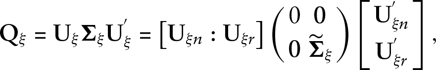
or its reparameterized version

where the columns of

where

Note that in practice,
Now suppose that for each small area or district

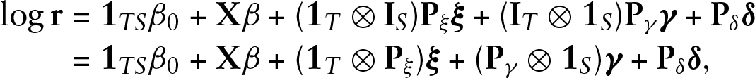
where the log relative risk is now modelled as

Here,

where

where
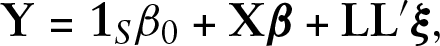
Similar to the spatial case, the spatio-temporal Model (2.4) can be expressed in matrix form as

where

which overcomes identifiability issues. For more details about this reparameterization, a generalization to RW2 priors for time, and the other interaction types described by Knorr-Held (2000), the reader is referred to Goicoa et al.(2018)Goicoa, Adin, Ugarte, and Hodges, where sum-to-zero constraints are alternatively derived to achieve model identifiability.
Confounding issues are more challenging in spatio-temporal settings than in spatial settings. In a spatio-temporal model, the covariates can exhibit spatial patterns each year, or temporal patterns in each area. As the model includes both spatial and temporal random effects along with interaction terms, the source of confounding can be spatial, temporal, or both. Note that the reparameterized Model (2.6) may present confounding problems as the covariates may be collinear with the design matrix of the spatial, temporal, or spatio-temporal random effects. The following section proposes two methods to alleviate confounding in spatio-temporal models, restricted spatial regression and constraints that make the estimated random effects orthogonal to the fixed effects.
Constraints can be used to make the random effects orthogonal to the fixed effects and, thus, alleviate confounding. The idea of inducing orthogonality between the fixed and random effects is similar to restricted regression, but they have some differences that can lead to notably distinct results. This section shows that constraining the random effects to be orthogonal to the fixed effects is not equivalent to removing from the linear predictor the component of the random effects in the span of the fixed effects, as might reasonably be assumed. In some cases, these differences are hardly noticeable in the spatial case but they become important in spatio-temporal settings.
Model reparameterization and restricted regression
Consider Model (2.6). This reparameterized spatio-temporal model is convenient as it solves the identifiability problems by removing repeated terms in the spatial and temporal main effects and the interaction random effects. The confounding issues are more challenging now because covariates are spatio-temporal, so we can have collinearity between the covariates and the spatial term, the covariates and the temporal term, or the covariates and the spatio-temporal interaction. Another concern is how to assess these correlations as the covariates have
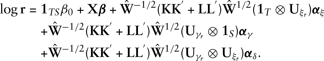
As the terms involving the matrix

Model (3.1) deserves comment. First, by using the matrix
Placing constraints is a way to achieve identifiability in spatio-temporal disease mapping models (Goicoa et al.(2018)Goicoa, Adin, Ugarte, and Hodges). Constraints can be used not just to identify models but also to alleviate spatial confounding, by constraining the random effects to be orthogonal to the fixed effects. This section considers such constraints. Specifically, consider Model (2.4) and consider the linear predictor

To make the random effects orthogonal to the fixed effects, these constraints are required:
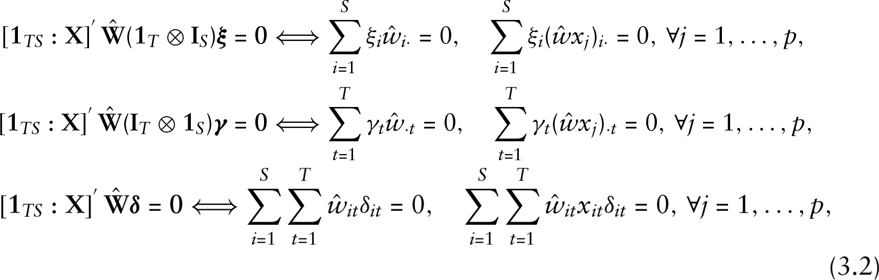
where
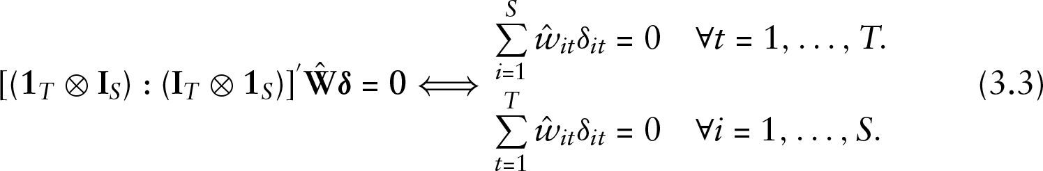
making the constraint
Though the restricted regression and the constraints approaches would seem to be equivalent, they are in fact different. The restricted regression approach focuses on the reduced Model (3.1), where the part of the random effects in the span of the fixed effects has been removed, and orthogonality is achieved through the matrix
One may think the methods are equivalent because removing the part of the random effects in the span of the fixed effects means
where

are made to be, respectively, oblique projections onto the orthogonal complements of the row spaces of the matrices

by setting Lξ to be the matrix whose columns are the eigenvectors with non-zero eigenvalues of the projection matrix
Two main methods have been used to fit spatial and spatio-temporal disease mapping models: a fully Bayesian approach and an empirical Bayes approach. The latter provides point estimates of quantities of interest, traditionally using penalized quasi-likelihood (PQL; Breslow and Clayton (1993)). It has proven to be interesting because it is relatively simple and has few convergence problems, and it has been used to fit different models such as the ICAR or P-splines (Dean et al.(2001)Dean, Ugarte, and Militino; Dean et al.(2004)Dean, Ugarte, and Militino; Ugarte et al.(2010)Ugarte, Goicoa, and Militino; Ugarte et al.(2012)Ugarte, Goicoa, Etxeberria, and Militino). However, PQL automatically places sum-to-zero constraints due to the rank deficiency of the random effects covariance matrices, and placing additional constraints is not so straightforward (see the Appendix for full details).
The fully Bayesian approach is probably the most-used technique for model fitting and inference because it provides a full posterior distribution for quantities of interest. Though it has traditionally relied on Markov chain Monte Carlo (MCMC), the computational burden of MCMC prompted development of other attractive procedures, including INLA (integrated nested Laplace approximations; Rue et al.(2009)Rue, Martino, and Chopin). INLA's main advantage is that it provides approximate Bayesian inference without using MCMC, leading to substantial reduction in computational cost. INLA is ready to use in the free software
Data analysis: The association between dowry deaths and socio-demographic covariates in Uttar Pradesh, India
In this section, the two approaches to alleviate confounding are used to assess the potential association between dowry deaths and some socio-demographic covariates in Uttar Pradesh, the most populated state in India. Dowry deaths is a cruel form of violence against women deep-rooted in India. It is strongly related to dowry, which can be defined as the amount of money, property, or goods that the bride's family gives to the groom or his relatives for the marriage. Although dowry was originally designed to protect women from unfair traditions, such as the impossibility of women owning immovable property (see Banerjee (2014)), it has become a means by which the husband or husband's relatives extort higher dowries under the threat of physical violence against the wife. This form of violence can be extended over time, ending in what is known as a dowry death. If a woman commits suicide because she has experienced mental or physical violence related to the dowry, this is also considered a dowry death.
We have data on dowry deaths in 70 districts of Uttar Pradesh, the Indian state with the highest rate of dowry deaths, during the period 2001–2014. In 2014, the last year of the study period, 8 455 dowry deaths were registered representing 29.2% of all dowry deaths in India. One of the difficulties of combatting this crime against women is the lack of knowledge about potential risk factors that might be associated with dowry deaths, and thus help to predict this crime. One hypothesized risk factor is the sex ratio, that is, the number of females per 1 000 males. The literature has contradictory results about the sex ratio: some authors find a negative association between dowry deaths and sex ratio (Mukherjee et al.(2001)Mukherjee, Rustagi, and Krishnaji), while others find a positive association (Dang et al.(2018)Dang, Kulkarni, and Gaiha). In a more in-depth study of dowry deaths in Uttar Pradesh, Vicente et al.(2020)Vicente, Goicoa, Fernandez-Rasines, and Ugarte consider spatio-temporal models and include some potential risk factors as covariates to assess their association with dowry deaths. However, these authors do not address confounding issues. We now focus on some of those covariates, namely sex ratio (
Data analysis
For purely spatial models, Reich et al.(2006)Reich, Hodges, and Zadnik and Hodges and Reich (2010) argued that spatial confounding is created by a high correlation between a covariate and the eigenvector of the spatial precision matrix having the smallest non-null eigenvalue. In the spatio-temporal setting, this suggests examining analogous correlations for the spatial, temporal, and spatio-temporal random effects. Therefore, before fitting any models, we examine the data and compute some correlations. Specifically, we split the covariates into spatial vectors for each year of the period, and computed Pearson's correlation between those spatial vectors and
Now we consider four spatio-temporal models.
Model ST1: Simple spatio-temporal Poisson model (Equation (2.4) without random effects) Model ST2: Spatio-temporal model without accounting for confounding (Equations (2.4) and (2.6) for INLA and PQL respectively). Model ST3: Spatio-temporal model with restricted regression (Equation (3.1)). Model ST4: Spatio-temporal model with orthogonality constraints (Equations (3.2) and (3.3))
Within the full Bayesian approach, we have used Normal prior distributions with mean 0 and variance equal to 1 000 for fixed effects. Regarding random effects, we have used uniform prior distributions on the positive real line for the standard deviations. We have also considered logGamma(1,0.00005) priors for the log-precisions and PC priors for the standard deviations (see, e.g., Simpson et al.(2017)Simpson, Rue, Riebler, Martins, and Sørbye), but these gave similar results and hence they are not shown here to save space.
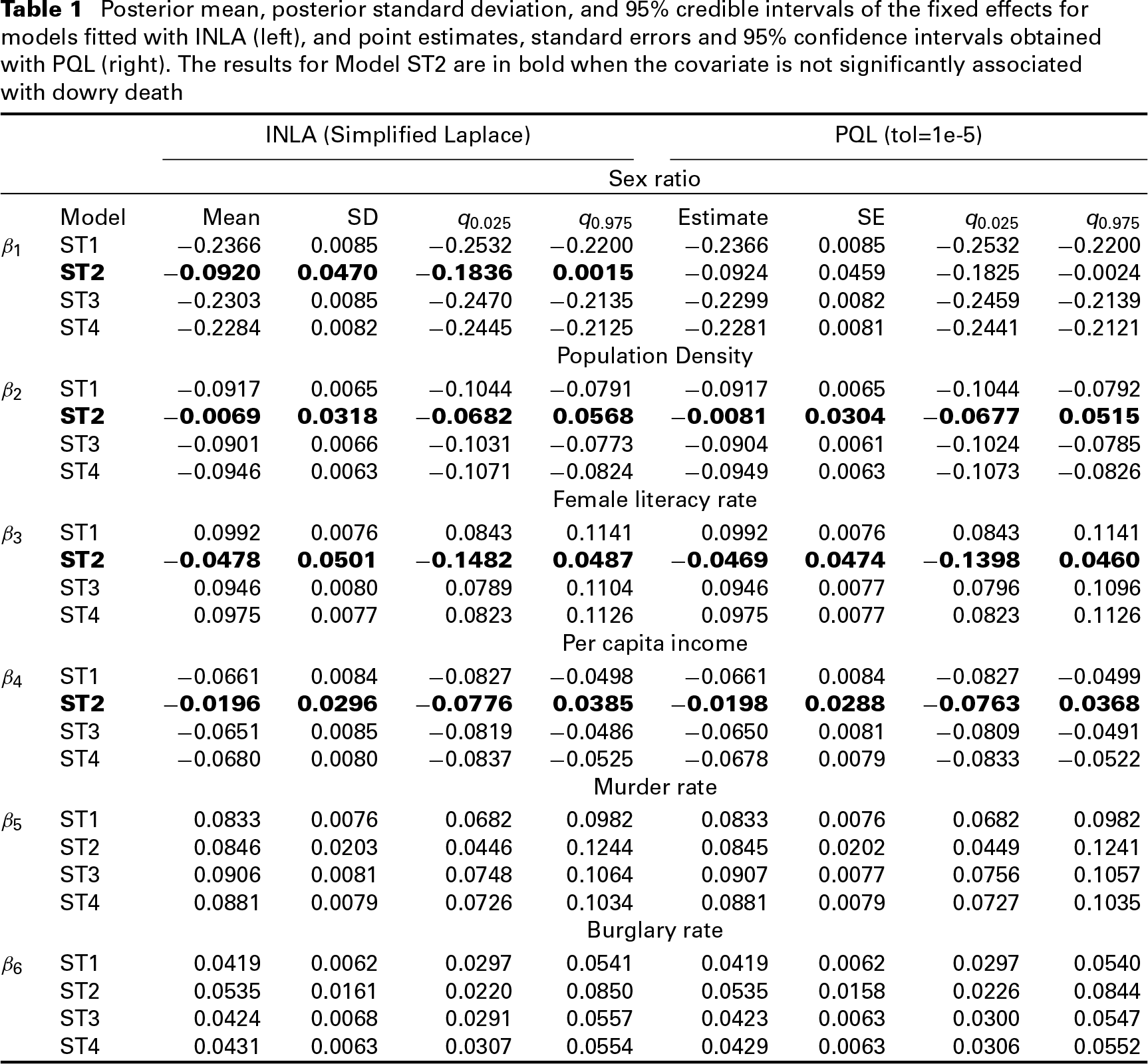
Posterior mean, posterior standard deviation, and 95% credible intervals of the fixed effects for models fitted with INLA (left), and point estimates, standard errors and 95% confidence intervals obtained with PQL (right). The results for Model ST2 are in bold when the covariate is not significantly associated with dowry death
Posterior mean, posterior standard deviation, and 95% credible intervals of the fixed effects for models fitted with INLA (left), and point estimates, standard errors and 95% confidence intervals obtained with PQL (right). The results for Model ST2 are in bold when the covariate is not significantly associated with dowry death
Table 1 shows the posterior mean and standard deviation of the fixed effects with a 95% credible interval, computed using INLA (simplified Laplace strategy). Point estimates obtained with PQL are also displayed with their standard error and 95% confidence interval. For sex ratio, the estimate with Model ST2 and INLA is about 40% (in absolute value) of the estimates obtained with Models ST1, ST3, and ST4, and the posterior SD is 5.5 times higher. For Model ST2, the 95% credible interval includes 0, while the intervals from the other models are far from zero. The results with PQL are similar although Model ST2’s confidence interval for sex ratio barely excludes 0. For population density, the estimate from Model ST2 is less than 10% of the estimates obtained with Models ST1, ST3, and ST4, with INLA or PQL, and again the posterior SD with Model ST2 is about 5 times higher than with the other models. The consequence is that using Model ST2, the association between population density and dowry deaths is not significant. Per capita income has similar results. The effect of confounding on the estimated association with female literacy rate is also noteworthy: with Model ST2, the estimated effect is negative (though not significant) whereas with the rest of models is positive and significant. The estimated associations with murder rate and burglary rate are similar for the four models, though the posterior SD is clearly larger for Model ST2. These results are revealing and illustrate the potential harmful consequences of ignoring the effects of confounding: the estimated association between the response and the covariate may be diluted or dramatically changed. Posterior estimates of the hyperparameters (standard deviations) are displayed in Table B.1 in Supplementary Material B. Similar estimates for the standard deviations are obtained with Models ST2, ST3, and ST4.
Model selection criteria and computing time (seconds) for spatio-temporal models fit with INLA and PQL. Computations were made on a twin superserver with four processors, Intel Xeon 6C and 96GB RAM, using the R-INLA (stable) version 19.09.03.
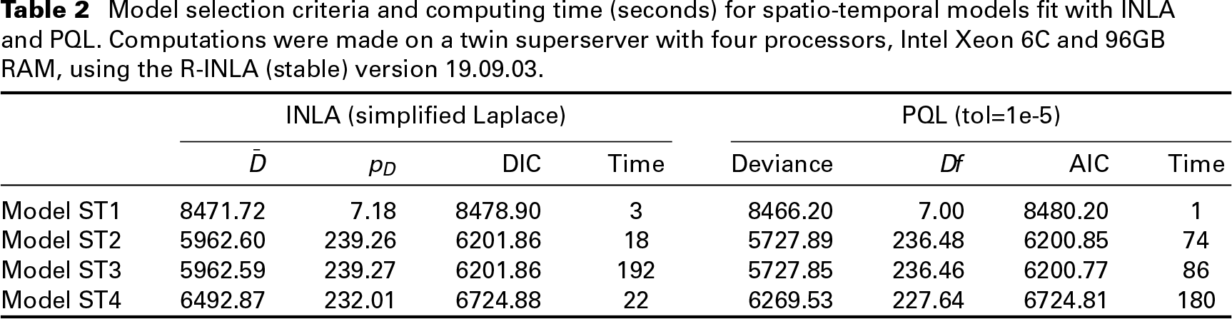
Spatio-temporal models accounting for confounding (Models ST3 and ST4) lead to similar estimates of the fixed effects and their posterior standard deviations but they differ in terms of model selection criteria. Table 2 displays the mean deviance (
Why do Models ST3 and ST4 fit so differently? First, the spatial and temporal terms in Models ST4 are
Finally, note that we also fit Model ST3 without premultiplying the temporal and spatio-temporal effects by
Including spatially correlated random effects in a model can seriously affect inference about fixed effects due to confounding. This is particularly dramatic in ecological spatial regression where the main objective is to estimate associations between the response variable and certain covariates. These relationships can be masked due to bias and variance inflation of the fixed effects caused by confounding. Though documented in the literature, spatial confounding has generally been ignored in applications and this practice has carried over to spatio-temporal settings. Here we study confounding in spatio-temporal ecological models in which including temporally correlated random effects and space-time interaction random effects (spatially and temporally correlated) can exacerbate confounding problems. We have considered two procedures to remedy the potentially harmful effects of confounding, restricted regression and constraints.
In light of this article's results, we would like to emphasize some points and provide some guidelines to practitioners. First, the relative risk estimates are not affected by confounding, so if the relative risks are of primary interest, ignoring confounding is not a problem. Second, both restricted regression and orthogonal constraints alleviate confounding and provide rather similar estimates of the fixed effects and their standard errors. However, the two approaches differ importantly in terms of model selection criteria and computing time. Although the constraints approach is computationally more efficient than restricted regression (in INLA), the latter gives clearly better fits. Consequently, if the target of the analysis is to establish associations between risk factors and the phenomenon under study, along with studying spatio-temporal patterns of risk, we recommend using restricted regression. We have also observed that differences between the approaches become more evident as the number of covariates increases. The difference in fits may arise because the deviance, and hence DIC (and AIC), are directly related to the orthogonal projection, the projection used in restricted regression. Because the orthogonal projection minimizes least squares, and
A desirable property of the constrained approach is that it keeps the (random) spatial and temporal main effects constant in time and space respectively while restricting all random effects to be orthogonal to the fixed effects. However, at least in the dataset analysed here, this behaviour comes at an important price in terms of model fit, unlike other proposals such as, for example, Hughes and Haran (2013). It is not easy to guess when the constrained and restricted regression approaches will lead to similar fits. We suspect that if the covariates do not have a substantial spatio-temporal interaction the constrained approached could work well. This is consistent with the observation that in a spatial analysis of our data for the year 2011 (not shown), both procedures are nearly equivalent. Moreover, fitting spatio-temporal models including only female literacy rate (a covariate with scarcely any spatio-temporal interaction), the difference in fit between both approaches is reduced considerably.
Both procedures have been fitted using a fully Bayesian and a classical approach. Though INLA provides the posterior distributions of all quantities and hence the maximum information, PQL is still a valuable tool that allows model fitting in a reasonable time providing essential information to understand the phenomenon under study. Computing times for restricted regression can be reduced in INLA by plugging in as initial values the posterior modes of the hyperparameters obtained from the spatio-temporal model with confounding. Similarly, restricted regression can be sped up in PQL by using as initial values the variance parameter estimates obtained from the spatio-temporal model with confounding.
To sum up, models with spatial, temporal, and spatio-temporal random effects lead to a good fit of the spatio-temporal patterns of risk, but they fail to account for the correct linear association between the response and the covariates. Models including only covariates provide unbiased estimates of the fixed effects coefficients but they give a poor fit as they do not capture the variability unexplained by the covariates. The restricted regression considered in this article offers in one single model the best of the two approaches: similar to the model without random effects, it provides correct estimates of the fixed effects but substantially improves model fit and prediction of spatio-temporal patterns of risk in line with the model with random effects. This is an advantage of the restricted regression approach over the models without random effects and classical spatio-temporal models. Recent research (Khan and Calder (2020)) concludes that for Gaussian models credible intervals for fixed effects obtained with restricted regression are nested within credible intervals obtained with models without spatial random effects. These authors acknowledge that restricted regression inference on the coefficients is very similar to the one from non-spatial models. In the Poisson spatio-temporal case study analysed here, credible intervals for some of the coefficients in the restricted regression approach are not nested within those of the model without random effects, but differences are small. Further research is needed to investigate this issue more in depth. The use of constraints also provides correct estimates of the fixed effects and improves model fit, but to a lesser extent than the restricted regression approach, at least in the dataset analysed here. We would like to highlight that in this work, associations between the covariates and the response should be understood as correlations, with the final objective of identifying good predictors of the response, and not as causal relationships within a causal-inference framework. This latter approach is beyond the scope of this article.
Finally, we want to emphasize the consequences of ignoring confounding for the data analysed here. Dowry death in India, particularly in Uttar Pradesh, is a complex problem for which risk factors (socio-demographic, economic, cultural or religious) are not yet clearly identified. Ignoring confounding may lead researchers to discard some potential risk factors and wrongly estimate their associations with dowry death. In this article, sex ratio, population density, female literacy rate, per capita income, murder rate, and burglary rate were found to be associated with dowry deaths when confounding was taken into account. Ignoring such effects masks the association between dowry deaths and some of those risk factors, which obscures understanding of this atrocious practice that takes the lives of thousands of women in India.
Appendix
This subsection is about adding orthogonality constraints in the PQL approach, in particular about modifying the algorithm to replace the sum-to-zero identifiability constraints with new constraints that identify the model and also achieve the desired orthogonality. Here we use ‘conditioning by kriging’ (pp. 37, 93 Rue and Held (2005)) where the covariance matrix of the random effects conditional on the constraints is used. Consider the covariance matrices
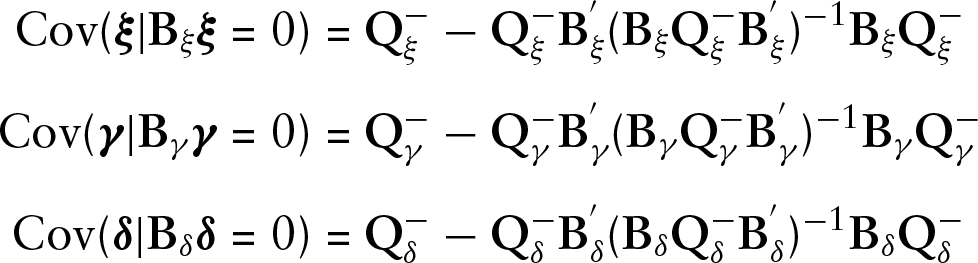
where ‘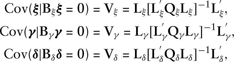
where 
where 
Clearly,
Footnotes
Supplementary materials
Supplementary materials for this article are available from
Declaration of Conflicting Interests
The authors declared no potential conflicts of interest with respect to the research, authorship and/or publication of this article.
Funding
The authors disclosed receipt of the following financial support for the research, authorship and/or publication of this article:
Acknowledgements
This work has been supported by Project MTM2017-82553-R (AEI/FEDER, UE). It has also been partially funded by ‘la Caixa’ Foundation (ID 1000010434), Caja Navarra Foundation, and UNED Pamplona, under agreement LCF/PR/PR15/51100007.
Software
Software in the form of R code, together with a sample input dataset and complete documentation will be available at