Does the single-walled carbon nanotube affect the rate constant of binding of biotin to streptavidin? Molecular dynamics simulation perspective

Abstract

The interaction of biotin and streptavidin in the presence and absence of a carbon nanotube was studied by molecular dynamics simulation. With respect to the Arrhenius dependence of the rate constants with temperature, those of streptavidin–biotin complex formation ( $k_1$ ) and streptavidin–biotin complex dissociation ( $k_{-1}$ ) were calculated from molecular dynamics simulation trajectories. Nanotube has reduced the amount of and k₁ and k₁. However, the biotin position in streptavidin does not change much. The results obtained from MMPBSA calculations show that the contribution of the van der Waals forces to both systems (in the absence and presence of the nanotube) was greater than that of electrostatic forces. The presence of the nanotube also led to the reduction of van der Waals and electrostatic forces in the interaction of biotin with streptavidin. However, this reduction was greater for electrostatic forces. In the absence of a nanotube, there are four hydrogen bonds between streptavidin and biotin, which are related to the residues Ser27, Tyr43, Ser45 and Ser88. In the presence of the nanotube, the hydrogen bonding of biotin with Ser45 is removed.

Introduction

In the biotin structure, there are amine, carboxylic, carbonyl and sulfur functional groups. Also in this molecule there are two five-membered heterocyclic rings. ¹ Thus, biotin is susceptible to interacting with proteins through hydrogen bonds and electrostatic interactions. One of the proteins that have a strong interaction with biotin is streptavidin. The interaction between biotin and streptavidin is one of the strongest physical bonds. ² For several reasons, the interaction of biotin with streptavidin is stronger than that of biotin with other proteins. First of all, there is the complementary structure of the biotin binding site in streptavidin with the shape of biotin. Also, at the binding site of biotin in streptavidin, a hydrogen bonding network is created between the biotin and the protein residues. This network of hydrogen bonds is composed of two layers. In the first layer, eight residues involving Asn23, Tyr43, Ser27, Ser45, Asn49, Ser88, Thr90 and Asp128 have a hydrogen bond with biotin. The second layer residues interact with the first shell residues. The presence of tryptophan in streptavidin leads to an increase in hydrophobic interactions and van der Waals interactions with biotin. Finally, the existence of a loop-shaped structure at the mouth of the biotin binding site acts as a lid and makes separation of biotin difficult. ³ This feature has made biotin widely used in biotechnology for biochemical identification.^4,5 Sélo et al. used a biotin–streptavidin identifier to identify synthetic peptides at different pH. ⁶ They showed that, when biotinylation occurred at the N-terminal extremity of immobilized peptides, the highest levels of binding were measured. Forrester et al. used the biotin–streptavidin interaction for S-nitrosylated proteins in biological samples. ⁷ Rehák et al. used streptavidin–biotin technology to prepare a mini biosensor to detect xanthine. The biosensor detection limit is 0.02 mmol L^–1 and its shelf life is five days.

Immobilization of proteins on different surfaces is common in order to increase their efficacy. ⁹ This technique has provided numerous examples of successful preparations with use in immunodiagnostics, ¹⁰ sensor preparation ¹¹ and enzyme reactors. ¹² It is important to maintain protein activity in protein fixation on the surface. Protein selectivity should also be maintained during the immobilization process. On the other hand, protein immobilization on a solid surface facilitates protein recovery. Due to their high surface area, the unique mechanical properties and specific electrical properties, carbon nanotubes can be functionalized with various functional groups. Functional groups such as amine, ¹³ carboxylic acid, ¹⁴ hydroxyl, ¹⁵ and epoxide ¹⁶ are among the well-known substituents. The diversity of functional groups and the variety of sites for the creation of substituents on carbon nanotubes has contributed to the process of targeted immobilization of proteins on their surface. Thus, carbon nanotubes are widely used candidates for protein immobilization. Streptavidin immobilized on functionalized carbon nanotubes has been used to detect various materials. Lai et al. used the streptavidin–carbon nanotube complex to identify tumor markers. They used $\alpha$ -fetoprotein and carcinoembryonic antigen as model analytes, and showed that this method offers suitable precision and wide linear ranges over four orders of magnitude with detection limits down to 0.061 and 0.093 pg mL⁻¹, respectively. ¹⁷ Keren et al. have used the combination of streptavidin–carbon nanotube–DNA to design a transistor. They report the substantiation of a self-assembled carbon nanotube field-effect transistor operating at room temperature. ¹⁸

In this article, molecular dynamics (MD) simulation was used to investigate the effect of a single-walled carbon nanotube (SWNT) on the rate constant of binding of biotin to streptavidin.

Computational details

The crystal structure of streptavidin (PDB: 1STP) was retrieved from the Protein Data Bank. ³ Two simulation boxes with dimensions of $7\times 7\times 7\mathrm{n}{\mathrm{m}}^3$ were defined. Streptavidin was located in the center of the boxes. Then, a nanotube molecule was randomly placed in one of the boxes. The simulation boxes were then filled with TIP3P water. ¹⁹ In order to neutralize the systems, an appropriate number of Na⁺ ions were added to each box. The OPLSAA force field was assigned for the SWNT, biotin and protein. Since the parameters of the OPLSAA for the SWNT and biotin have not been incorporated with in GROMACS ²⁰ by default, these parameters were inserted manually. To do this, the geometry of the SWNT was optimized using the Beck–Lee–Young–Parr exchange correlation functional (B3LYP) ²¹ as implemented in the Gaussian 03 program. ²² The 6-311+G(d,p) basis set was employed. The optimized geometry was confirmed to have no imaginary frequency of the Hessian. The optimized structure was visualized using the Chemcraft 1.5 program. ²³ To minimize the energy of the whole system and to relax the solvent molecules, the steepest descent algorithm was used and periodic boundary conditions were used. Further, to maintain equilibrium in the designed systems, simulations were performed for 1000 ps using NVT and NPT ensembles, respectively. Finally, each system was simulated with a time step of 2 fs for 30000 ps.

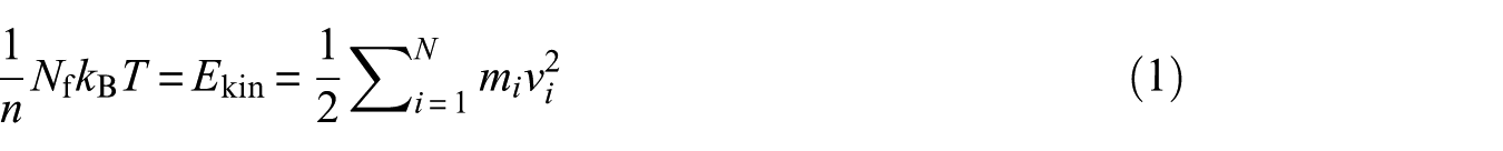
In MD simulation the temperature is given by the total kinetic energy of the N-particle system:

$$\frac{1}{n}{N}_{\mathrm{f}}{k}_{\mathrm{B}}T=E_{\mathrm{kin}}=\frac{1}{2}\sum _{i=1}^N{m}_i{v}_i^2$$

(1)

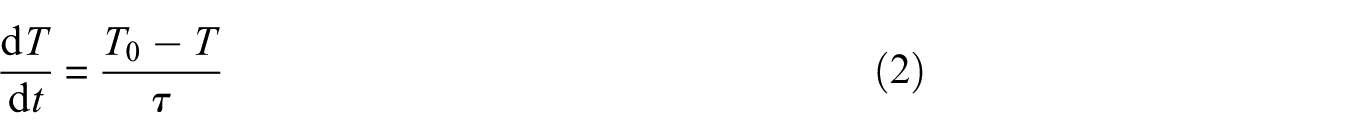
Where $k_{\mathrm{B}}$ is Boltzmann’s constant and $N_{\mathrm{f}}$ is the number of degrees of freedom. On the other hand, MD simulation is solving Newton’s second law for a multi-particle system. E_kin, m_i, v_i and n is total kinetics energy, atomic mass, mass velocity and number of molecular dynamics simulation trajectories, respectively. In a system with particles of different masses, the same force is applied to the particles causing different kinetic energies. Lighter particles tend to have more kinetic energy and larger particles have less kinetic energy. This phenomenon is referred to as "hot solvent–cold solute". ²⁴ There are several other reasons why it might be necessary to control the temperature of the system such as drift during equilibration, drift as a result of force truncation, integration errors and heating due to external or frictional forces. However, from a thermodynamic point of view, it may only lead to an increase in temperature, but retains its physical meaning. ²⁵ To control the temperature (T) and correct its deviation from temperature $T_0$ , the following equation is used

$$\frac{\mathrm{d}T}{\mathrm{d}t}=\frac{T_0-T}{\tau }$$

(2)

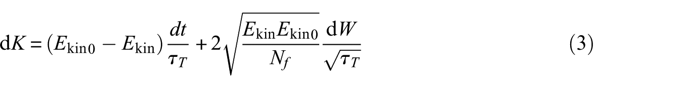
which means that a temperature deviation decays exponentially with a time constant $\tau$ . T₀ is reference temperature of system. This method of coupling has the advantage that the strength of the coupling can be varied and adapted to the user requirement: for equilibration purposes, the coupling time can be quite short, but for reliable equilibrium runs it can be much longer, in which case it hardly influences the conservative dynamics. Because this method suppresses the fluctuations of the kinetic energy, it does not generate a proper canonical ensemble so, rigorously, the sampling will be incorrect. To solve this problem, the algorithm V-rescale is used. The V-rescale method is essentially the above method with an additional stochastic term that ensures a correct kinetic energy distribution by modifying it according to

$$\mathrm{d}K=({E_{\mathrm{kin}}}_0-E_{\mathrm{kin}})\frac{\mathrm{dt}}{{\tau }_T}+2\sqrt{\frac{E_{\mathrm{kin}}{E_{\mathrm{kin}}}_0}{N_f}}\frac{\mathrm{d}W}{\sqrt{{\tau }_T}}$$

(3)

where $\mathrm{d}W$ is a Wiener process. dK is change in kinetic energy distribution. There are no additional parameters, except for a random seed.

The V-rescale coupling algorithm was employed to maintain various components at a constant temperature and pressure during simulations. ²⁶ The PME algorithm ²⁷ was used to determine the electrostatic interactions of each component of the systems. Covalent bonds present in the molecules were constrained using the LINCS algorithm ²⁸ and the chemical bonds in solvent molecules were held constant using the SETTLE algorithm. All MD calculations were performed using GROMACS 5.2.1.

Results and discussion

The following schematic was used to determine the rate constants of biotin binding to streptavidin.

$$\mathrm{streptavidin}+\mathrm{biotin}\begin{array}{c}\stackrel{k_1}{\to }\hfill \\ \multicolumn{1}{c}{\underset{k_{-1}}{\leftarrow }}\end{array}\mathrm{streptavidin}-\mathrm{biotin}$$

This schematic was considered once in the absence of the nanotube and once in the presence of the nanotube which were called systems A and B, respectively. Let $F_{\mathrm{bind}}\left(t\right)$ be a binary indicator of binding process, i.e. $F_{\mathrm{bind}}\left(t\right)=1$ corresponds to the trajectory being bound at time t, and $F_{\mathrm{bind}}\left(t\right)=0$ corresponds to a non-binding state. Also, assume one can determine $F_{\mathrm{bind}}\left(t\right)$ from each conformation in MD simulation trajectories. The $F_{\mathrm{bind}}\left(t\right)$ function can be the root-mean-square-deviation (RMSD) or radius of gyration (Rg). Here the RMSD quantity was used as an indicator. The amount of RMSD was assigned a cutoff that before and after this amount the streptavidin was considered as bonded and non-bonded with biotin, respectively. Using these definitions

$$\frac{\mathrm{d}{F}_{\mathrm{bind}}\left(t\right)}{\mathrm{d}t}=k_{-1}{F}_{\mathrm{non}-\mathrm{bind}}\left(t\right)-k_1{F}_{\mathrm{bind}}\left(t\right)$$

(4)

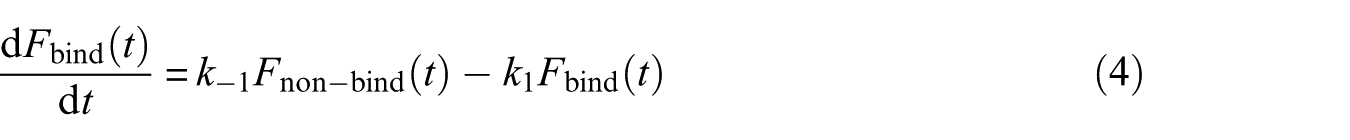
where $k_1$ and $k_{-1}$ are the rate constants of streptavidin–biotin complex formation and streptavidin–biotin complex dissociation, respectively. Then, with respect to the Arrhenius dependences of the rate constants with temperature

$$k_1=A_1{e}^{\frac{-E_{\mathrm{a},1}}{k_{\mathrm{B}}T}}{k}_{-1}=A_{-1}{e}^{\frac{-E_{\mathrm{a},-1}}{k_{\mathrm{B}}T}}$$

(5)

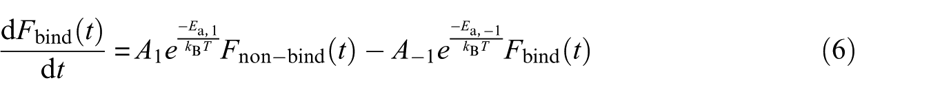
where $k_{\mathrm{B}}$ and T are Boltzmann’s constant and temperature, respectively. If we rewrite equation (4) with the explicit time dependences of temperature, we have for each trajectory

$$\frac{\mathrm{d}{F}_{\mathrm{bind}}\left(t\right)}{\mathrm{d}t}=A_1{e}^{\frac{-E_{\mathrm{a},1}}{k_{\mathrm{B}}T}}{F}_{\mathrm{non}-\mathrm{bind}}\left(t\right)-A_{-1}{e}^{\frac{-E_{\mathrm{a},-1}}{k_{\mathrm{B}}T}}{F}_{\mathrm{bind}}\left(t\right)$$

(6)

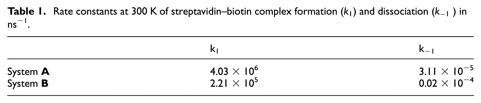
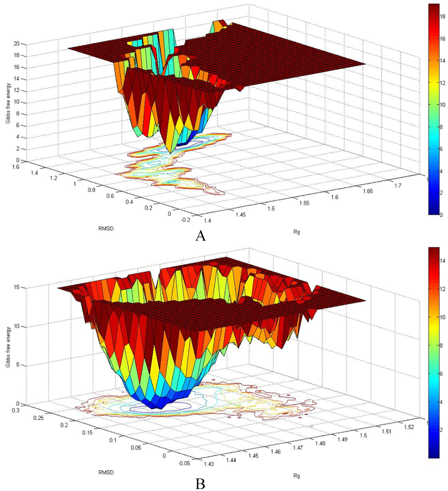
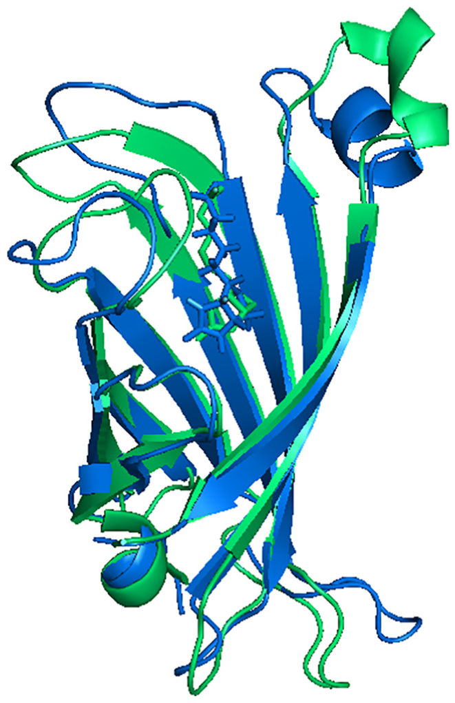
In equation (6), The k_BT expression is called beta; hence, the beta quantity $\left(\frac{1}{k_{\mathrm{B}}T}\right)$ changes stochastically with time. Thus, this equationcannot be integrated analytically. Thus, it was necessary to integrate it numerically. Given equations (4)–(6) and the RMSD-dependence of the time taken from the MD simulation trajectories, the rate constants were calculated and the results are listed in Table 1. Given the values reported in Table 1, the presence of the nanotube caused $k_1$ and $k_{-1}$ to decrease. On the other hand, the ratio of $k_1$ to $k_{-1}$ , which is equivalent to the formation constant of the streptavidin–biotin complex, is for the systems A and B of the order of ${10}^{11}$ and ${10}^9$ , respectively. These values are in agreement with the experimental dissociation constant of the streptavidin–biotin complex which is of the order of 10⁻¹¹–10⁻¹⁴ mol L⁻¹. ²⁹ For a closer look at the observed difference in the rate constant values in the presence of the nanotube, the structure of the streptavidin was sampled from the systems A and B. For the sampling of the structure, the free energy landscape (FEL) analysis method was used. ³⁰ Calculations of the RMSD and the Rg of streptavidin, obtaining the possible presence of the streptavidin configuration at every corresponding value of RMSD and Rg, and calculation of the free energy of configurations based on the probability values of the possible presence, are the three main stages of FEL analysis. The results of FEL analysis are shown in 3D diagrams in Figure 1. In these diagrams, the minimum areas of free energy are shown in blue. The diagrams show that there is a local minimum in the two systems A and B. That means streptavidin in the presence of biotin has a stable configuration in the presence and absence of the carbon nanotube. Samples were taken from the simulation time corresponding to the lowest free energy. The superimposed structures of streptavidin obtained by free energy analysis are shown in Figure 2. In this figure, the green and blue colors are related to the structure of streptavidin in the presence and absence of the nanotube, respectively. It is seen from the figure that the nanotube has a greater effect on the loop parts than the sheets. On the other hand, the nanotube has made the upper crater of the protein more closed. Also, in the presence of the nanotube, the biotin conformation has changed. However, its position in the streptavidin has not changed much. ³¹ The Kollman et al method was used ³² to evaluate the contribution of different forces to the interaction of biotin with streptavidin. In this method, the free energy is obtained by

$$G=E_{\mathrm{bnd}}+E_{\mathrm{el}}+E_{\mathrm{vdW}}+G_{\mathrm{pol}}+G_{\mathrm{np}}-\mathrm{TS}$$

(7)

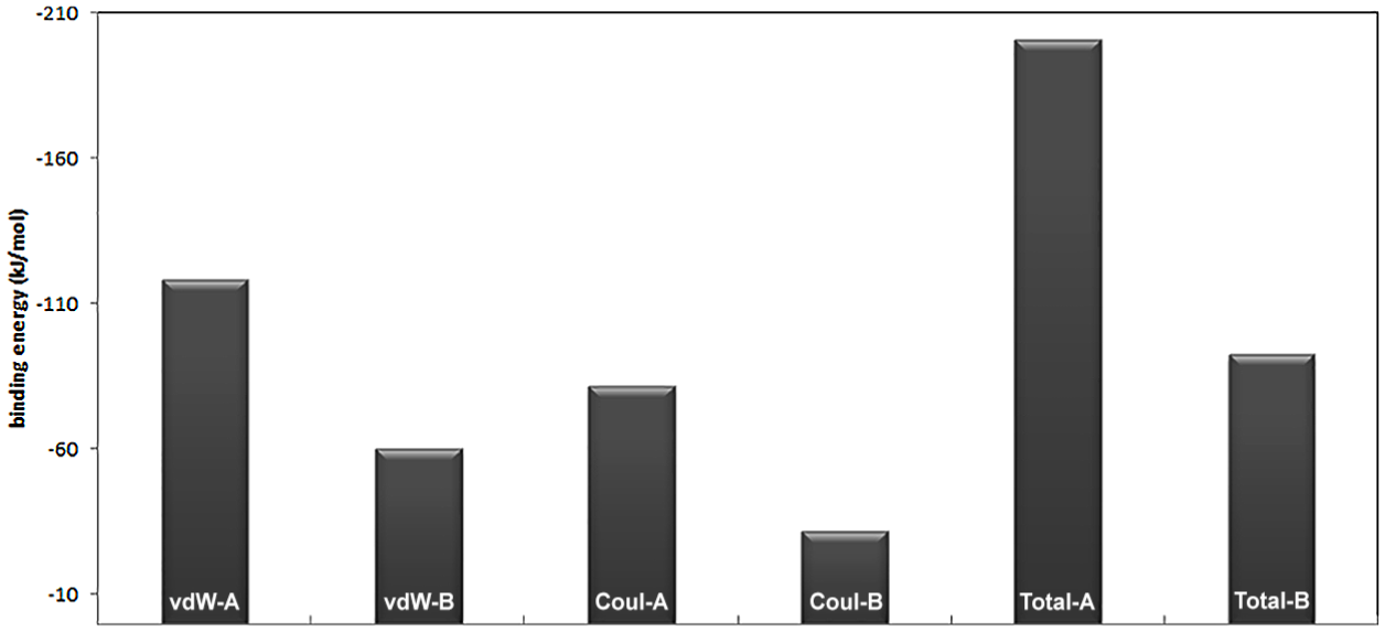
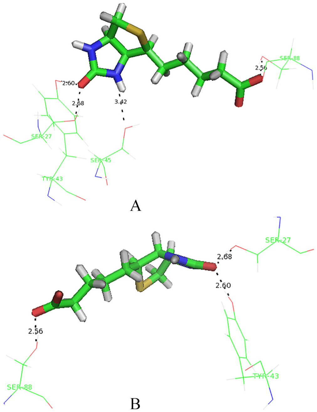
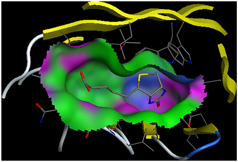
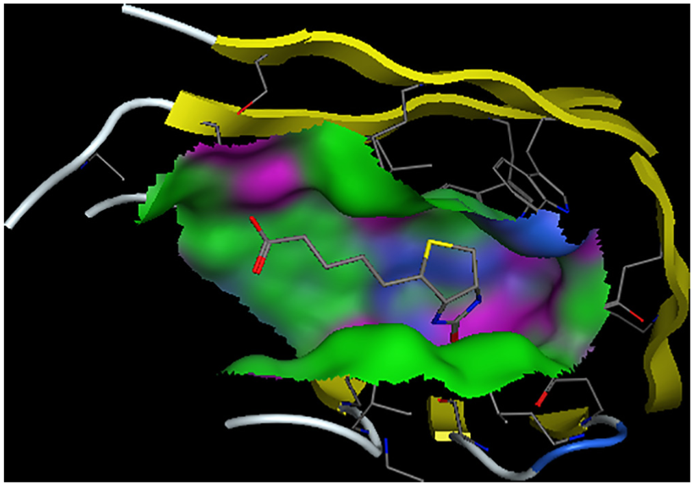
where $E_{\mathrm{bnd}},E_{\mathrm{el}}\mathrm{and}{E}_{\mathrm{vdW}}$ are the molecular mechanics energies (bonding, bending, and dihedral), electrostatic energy and van der Waals interactions, respectively; $G_{\mathrm{pol}}$ and $G_{\mathrm{np}}$ are polar and nonpolar solvation free energies, which were obtained from the generalized Born and solvent accessible surface methods, respectively. The last term in equation 7, in which T is temperature and S is entropy, was obtained from the normal mode analysis. The results of the Kollman method for the interaction of biotin and streptavidin in the presence of a nanotube (system B) and its absence (system A) are shown in Figure 3. According to the figure, the contribution of the van der Waals forces to both systems is greater than that of electrostatic forces. The presence of the nanotube has also led to the reduction of both van der Waals and electrostatic forces in the interaction of biotin with streptavidin. However, this reduction is greater for electrostatic forces. Streptavidin residues in the absence of the nanotube, which have hydrogen bonding with biotin, are shown in Figure 4. These residues are: Ser27, Tyr43, Ser45 and Ser88. In this figure, hydrogen bonds are shown as black dashed lines. Hydrogen bond lengths are also shown. Streptavidin residues in the presence of the nanotube, which have hydrogen bonding with biotin, are also shown in Figure 4. These residues are: Ser27, Tyr43 and Ser88. It is observed that in the presence of the nanotube, Ser45 is removed from the list of hydrogen bonded residues with biotin. In Figures 5 and 6, the binding site of biotin to streptavidin, in the absence of the nanotube and in the presence of the nanotubes, is shown, respectively. In these figures, hydrogen bond interactions, hydrophobic interactions and electrostatic interactions are shown in purple, green and blue, respectively. As one can see, the contribution of electrostatic interactions is lower than the rest. On the other hand, the shape of the β sheets has not been altered in the protein in the presence or absence of the nanotube.

Table 1.

Rate constants at 300 K of streptavidin–biotin complex formation ( $k_1$ ) and dissociation ( $k_{-1}$ ) in ns⁻¹.

	k1	k−1
System A	4.03 × 106	3.11 × 10−5
System B	2.21 × 105	0.02 × 10−4

Figure 1.

Free energy landscape of simulated system. A for absence of carbon nanotube and B for presence of carbon nanotube.

Figure 2.

Superimposed structures of streptavidin obtained from free energy landscape analysis. The green and blue colors are related to the structure of the streptavidin in the presence of the nanotube and the absence of the nanotube.

Figure 3.

Results of the MMPBSA method for the interaction of biotin and streptavidin in the presence of a nanotube (system B) and its absence (system A).

Figure 4.

Streptavidin residues which have a hydrogen bond with biotin. A for absence of carbon nanotube and B for presence of carbon nanotube.

Figure 5.

Biotin binding site in absence of carbon nanotube.

Figure 6.

Biotin binding site in presence of carbon nanotube.

Conclusion

In this work, MD simulation was used to calculate the rate constant of the biotin binding process to streptavidin. The effect of the carbon nanotube on the rate constant of binding of biotin to streptavidin was also investigated. For this purpose, the RMSD parameter was considered as a marker of the binding of biotin to streptavidin. The results showed that the nanotube reduced the magnitude of the rate constants. The secondary structure analysis also showed that the looped parts of the streptavidin were more affected by the nanotube than the sheet parts.