
Abstract
Aircraft contrails contribute to climate change through global radiative forcing. As part of the general effort aimed at developing reliable decision-making tools, this paper demonstrates the feasibility of implementing a Lagrangian ice microphysical module in a commercial CFD code to characterize the early development of near-field contrails. While engine jets are highly parameterized in most existing models in a way that neglects the nozzle exit-related aspects, our model accounts for the geometric complexity of modern turbofan exhausts. The modeling strategy is based on three-dimensional URANS simulations of an aircraft nozzle exit involving a bypass and a core jet (Eulerian gas phase). Solid soot and ice particles (dispersed phase) are individually tracked using a Lagrangian approach. The implemented microphysical module accounts for the main process of water-vapor condensation on pre-activated soot particles known as heterogeneous condensation. The predictive capabilities of the proposed model are demonstrated through a comprehensive validation set based on the jet-flow dynamics and turbulence statistics in the case of compressible, turbulent coaxial jets. Simulations of contrail formation from a realistic nozzle-exit geometry of the CFM56-3 engine (short-cowl nozzle delivering a dual stream jet with a bypass rate of 5.3) were also carried out in typical cruise flight conditions ensuring contrail formation. The model provides reliable predictions in terms of the plume dilution and ice-particle properties as compared to available in-flight and numerical data. Such a model can then be used to characterize the impact of nozzle-exit parameters on the optical and microphysical properties of near-field contrails.
Keywords
Introduction
The continuous growth in air passengers by about 5% per year has increased scientific concerns about the climate impact of commercial aviation. 1 Cruise flights contribute to global warming through soot and water-vapor emissions from aircraft engines that are responsible for visible white condensation trails (contrails) behind aircraft.2,3 Persistent contrails composed mainly of supersaturated ice crystals survive in the atmosphere for several hours and even evolve to form large cirrus formations referred to as aircraft-induced clouds (AIC). 4 The spreading and persistence of this artificial cloudiness in the atmosphere determine their impact on the earth’s radiative balance. 5 Global assessments 6 show that the impact of linear contrails is about 3–9·10−3 W·m−2, while the impact of AIC is 10 times higher, 6 which corresponds to three times the impact of aviation CO2 alone. 7 For this reason, the contrail formation process has been a topic of increasing interest in the literature. Owing to both complexity and onerous costs of in-flight measurements, the development of innovative mitigation strategies has to be based on reliable decision-making tools. As such, several modeling approaches with different levels of microphysics/dynamics representations have been used in literature to investigate contrails. The following is a short review of main approaches and findings.
Modeling contrail life cycle involves several scales ranging from local scales in the engine jet phase (t ~ 0–10 s after the exhaust emission) to the global scale in the dispersion phase (few minutes to hours after the exhaust emission; see Figure 1). From the thermodynamic point of view, the revised Schmidt–Appleman criterion 8 helps to determine atmospheric regions of contrail occurrence based on water liquid saturation conditions. This criterion was used to initiate contrail formation in global models, such as in the Contrail Cirrus Prediction Tool (CoCiP), 9 and made it possible to assess the global environmental impact of contrails. To allow coverage of the full evolution cycle of a large population of contrails, the physics modeling was relatively simplified, such as for initialization of the species concentration with a Gaussian profile. Even though the results of regional air-traffic simulations9,10 were quite consistent with in-flight measurements and satellite observations, the microphysical processes of ice production remain misunderstood. A more precise characterization of ice particles was achieved using 0-D microphysical trajectory box models.11,12 This class of models allows detailed chemical kinetics and microphysics in the engine jet phase. For instance, simulations of young contrails11,13 highlighted the domination of soot-induced heterogeneous freezing due to the large amount of emitted soot condensation nuclei from kerosene-fueled engines. In this respect, the reduction of soot emissions with the use of alternative jet fuels can help alter the optical properties of contrails. 14 The box model results for plume dilution, however, showed some discrepancies compared to in-flight measurements due to (1) the absence of a detailed turbulence modeling11,14 and (2) the simplified level of dynamics using averaged bulk exhaust (provided by semiempirical models).11,14 Some authors remedied the shortcomings through offline-coupling strategies with an external fluid-flow solver.15,16
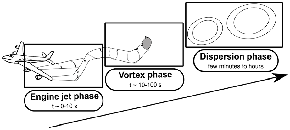
Evolution of a contrail in the wake of an aircraft.
In the last two decades, computational cost-effectiveness has increased interest in 3D CFD-based models to refine the early plume dynamics and associated mixing process. Early plume properties are known to influence later contrail stages (optical depth, radiative forcing) as shown by the studies on the engine jet and vortex phase.7,17 As such, they are usually used as inputs in mesoscale models.18,19 Solid particles motion can be tracked in CFD using either an Eulerian 20 or a Lagrangian.21–23 The former can capture the motion of higher particle concentrations 24 with either bulk parametrization25,26 or bins 20 for microphysics modeling. The simplest representation of particle-size distribution considers a single bin (monodisperse distribution) as used by Khou et al.27,28 who investigated the near-field contrails (engine jet phase) behind realistic commercial aircraft geometries using Reynolds-averaged Navier–Stokes (RANS) equations for turbulence modeling. Results revealed that wingtip vortices drained and cooled jets and highlighted the role of ambient relative humidity on ice-crystal properties. Using a single bin could, however, prevent accurate estimates of ice-crystal concentration. 28 The most physically accurate treatment of ice particles in Eulerian terms considers size-resolved (binned) microphysics, 20 which avoids the problems of numerical diffusion inherent in bulk models29,30 that could lead to slight discrepancies in the dispersion of ice and water-vapor fields. The computational cost, however, is excessive (see the detailed review 31 ).
In contrast, Lagrangian tracking allows for an explicit process-oriented modeling of ice microphysics, 30 which accounts for its popularity in contrail research for a while.15,22,30 Most if not all Lagrangian studies are highly parameterized in a way that neglects nozzle exit-related aspects. For example, Paoli et al. 32 modeled free turbulent jets with classical expansion laws to investigate contrail formation for two- and four-engine configurations. Unterstrasser and Görsch 33 also used Gaussian-like plume profiles to study the vortex phase and to characterize the impact of aircraft type on contrail evolution. These simplified representations of the nozzle exhaust jet do not allow for accurately taking into consideration the features of modern turbofan nozzles. As the flow structure and mixing in the early plume depend on engine exhaust parameters, the impact of high bypass rates and complex geometries (e.g. short and long cowls and chevrons) on the near-field microphysics remain unclear. This particularly motivated the development of a CFD-microphysical model that integrates the nozzle-exit geometry and avoids using parameterizations to describe the exhaust plume.
Therefore, the main objective of this study was to implement a Lagrangian microphysical module in a CFD code to simulate ice-particle growth in near-field contrails starting from a realistic turbofan nozzle exit. To the authors’ knowledge, no contrail study has integrated the actual nozzle-exit geometry in a Lagrangian approach. A high-resolution spatial unsteady RANS method was therefore used to demonstrate the feasibility of the present approach. The paper is organized as follows. Section 2 begins with a description of the modeling approach, followed by the mathematical equations of fluid dynamics, particle motion, and ice microphysics. Section 3 describes the model and presents how the microphysical module was coupled to Simcenter Star-CCM+ CFD software. Section 4 discusses the validation test results for jet dynamics, plume dilution, and ice-particle properties.
Model description
Approach for modeling the formation of near-field contrails
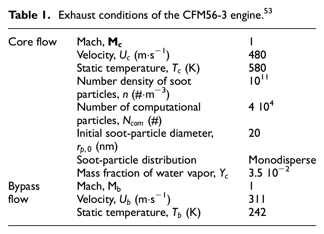
Figure 2 shows that the nozzle exit flow from a turbofan engine at cruise flight consists of two jets: a hot core flow and a surrounding cold bypass flow. Both jets are mixed with the freestream moist air. The bypass flow simply contains ambient moist air that has been slightly accelerated by the engine fan, while the core jet drives the fuel-combustion products composed of gaseous emissions laden with soot particles (dispersed or solid phase). Water vapor in the dilution plume condenses onto soot particles, which serve as condensation nuclei when activated with sulfuric acid (heterogeneous nucleation 11 ). Under saturation conditions, ice particles form and grow by taking up more condensable matter – that is, water vapor – from the plume and ambient air, leading to contrail formation.
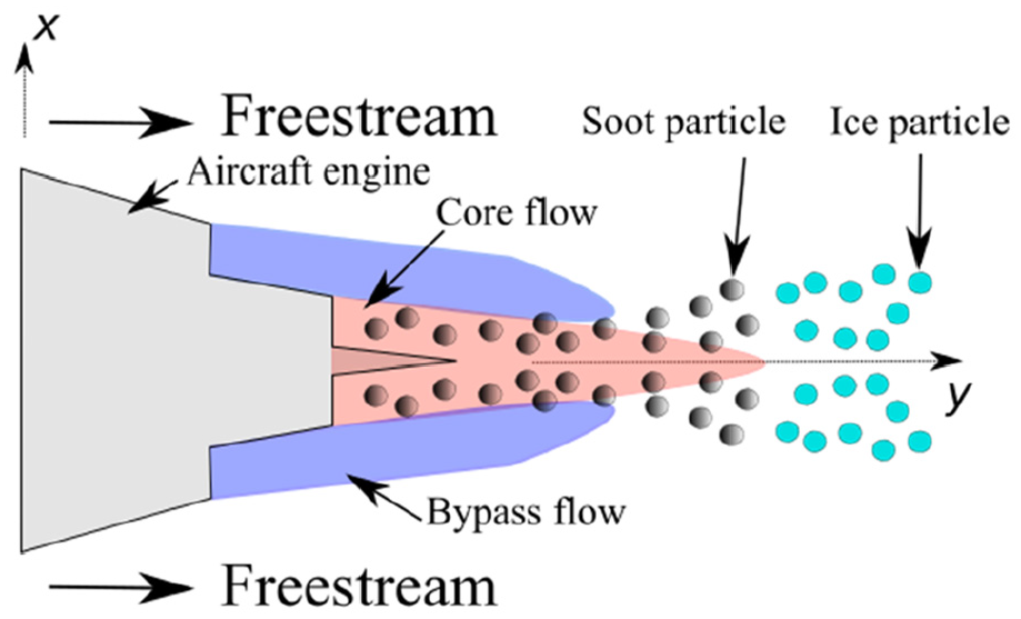
2D Scheme of exhaust flow from a turbofan engine with ice-particle formation.
In this study, the Eulerian–Lagrangian approach was used to model the formation of contrail ice particles in the near field of an aircraft engine. The continuous gas phase was modeled with the Eulerian approach, while the dispersed-phase of solid particles (soot and ice particles) were tracked with the Lagrangian approach. Lastly, a one-way microphysical coupling was considered to account for ice-particle growth due to water-vapor condensation.
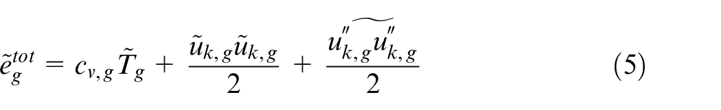
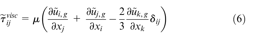
Gas-phase equations
The compressible flow of the gas phase (“g” index) is considered to be a mixture of two miscible species: air (“a” index) and water vapor (“w” index). Assuming an ideal gas, the mixture density

where
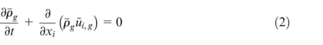
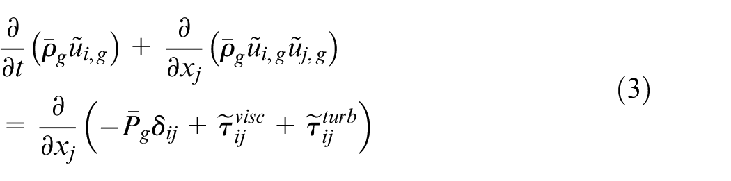
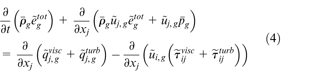
Solving equations (2)–(4) provides the primary variables of the mean flow
To compute the mixture composition in the gas phase (
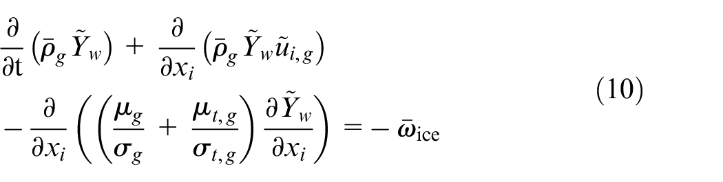

Equation (10) translates the mass conservation of water vapor where the source term
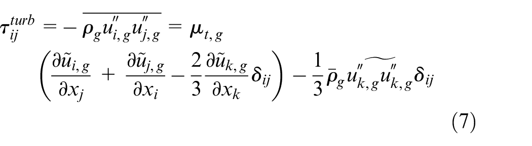
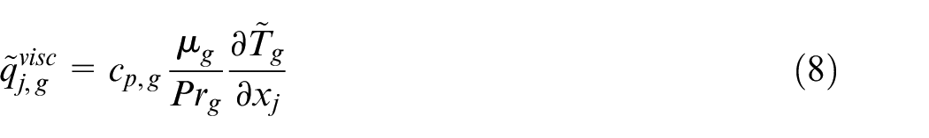
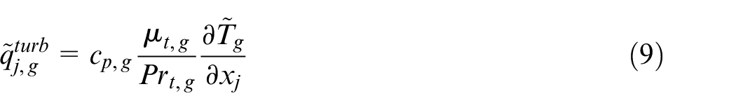
Lastly, the eddy viscosity
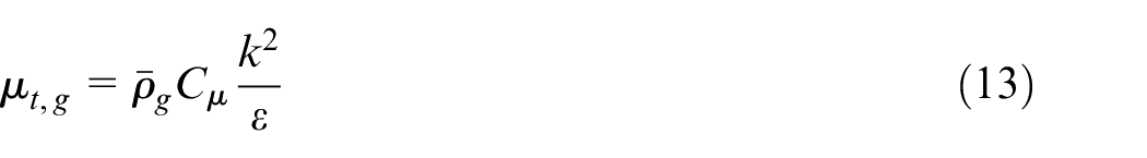
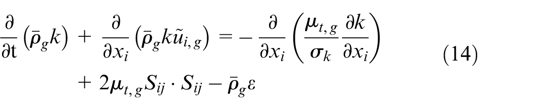
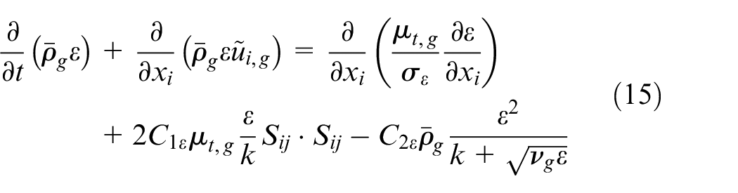
where
Dispersed-phase equations and microphysics model
Particles motion
At cruise conditions, the number density of physical particles is so high that a modeling simplification is required to save simulation time. For example, a typical value for emitted soot particles from an engine nozzle is about 1011 #· m−3.
39
Therefore, computational particles are considered as spheres of radius
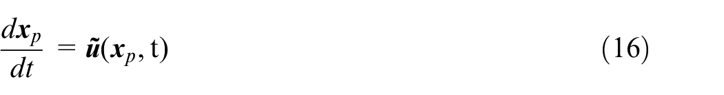
where
Ice-particle growth
In contrails, ice-particle growth is due to condensation of water vapor onto suitable nucleation sites on pre-activate particles (mostly soot particles).
8
The ratio between the local water vapor partial pressure (
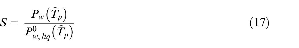
such as the local pressure

where
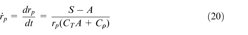
The mass change of a single-particle (computational) growth due to condensation/evaporation effects can be expressed by a diffusion law as described by the Fukuta and Walter 44 model, which describes the change of both particle mass and size as follows:
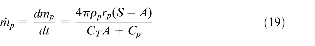
where
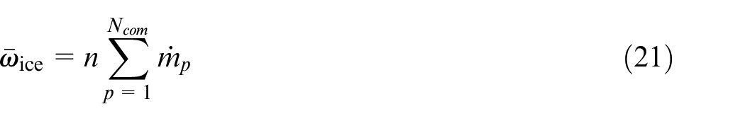
where n is the number density of particles contained in a volume cell V, such that
Numerical methodology
The CFD solver is based on a cell-centered finite-volume approach for unstructured grids.
20
The SIMPLE algorithm
45
was used to solve the flow governing equations. A second-order upwind scheme was used for space discretization, while time integration was achieved with a second-order Euler scheme. For the model of ice-particle growth, a fourth-order Runge-Kutta scheme was used to discretize the equation (20) of particle size change. The discretization of the equation (20) is presented in Appendix B. The microphysical module was implemented as a user-defined function in the commercial CFD code in Simcenter STAR-CCM+ v13.04. The script of the microphysical module (coded in C) can be downloaded from Ref.
46
The methodology for coupling with the CFD solver is detailed in Figure 3. At each time step, the primary flow variables of both gas- and dispersed-phase are derived from the CFD solver. The pressure and temperature at each grid point help to compute the thermodynamic variables (
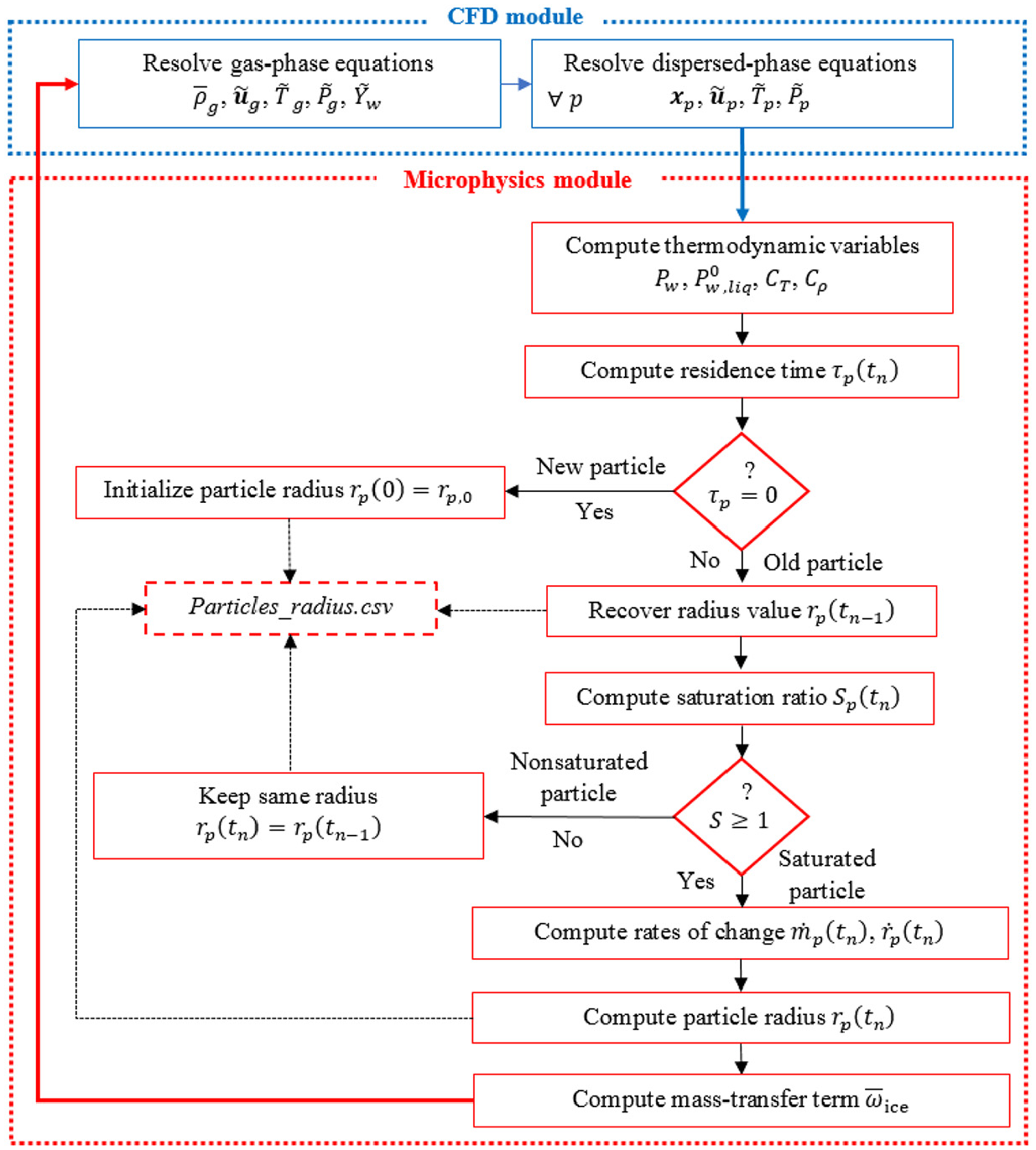
Schematic of the CFD-microphysics coupling for modeling ice-particle growth.
Validation tests and results
Two validation tests were performed to assess the reliability of the CFD-microphysics model presented above for studying ice-particle growth in the exhaust jet of an aircraft engine. In the first test, the model’s gas-phase resolution (i.e. jet dynamics and turbulence) was assessed with experimental results from the canonical case of compressible coaxial jets. This validation test made it possible to choose the most suitable turbulence model. In the second test, the model’s microphysical resolution in terms of dilution and ice-particle properties (size, distribution, optical depth) were assessed in the exhaust jet of a CFM56-3 engine at realistic cruise flight conditions.
Compressible coaxial turbulent jets
Computational domain and grid
Guitton et al.
47
experimentally characterized the flow dynamics and turbulence in the case of isothermal compressible coaxial jets of air. This experiment was used as a validation test case for our computational model. As shown in Figure 4, the nozzle had a length
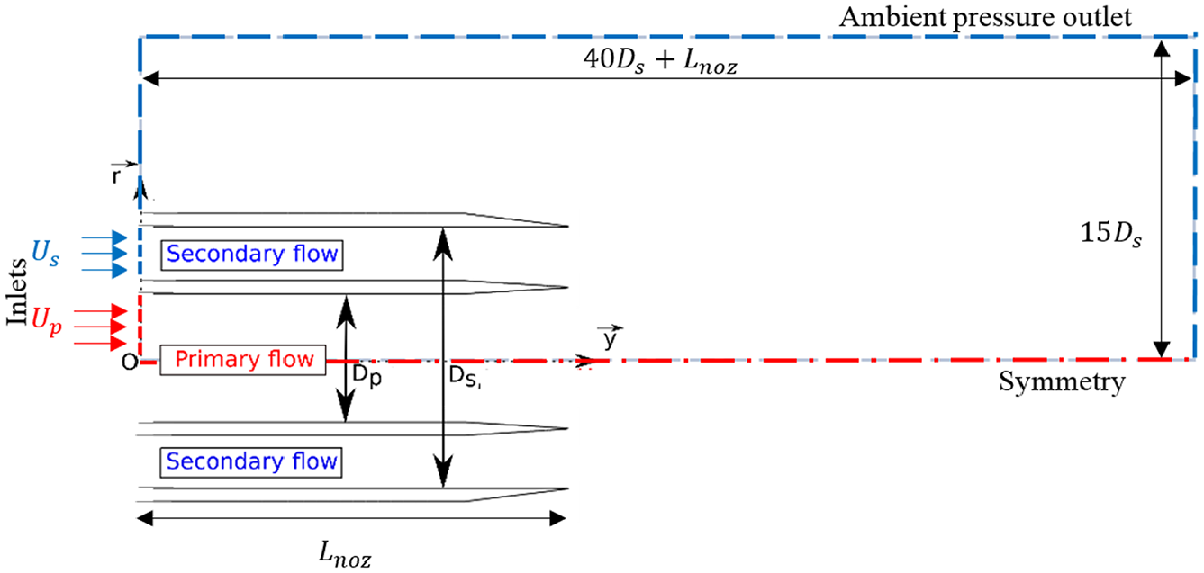
Scheme of the computational domain with nozzle geometry and boundary conditions.
A grid convergence study was carried out using three grids: coarse (290,110 cells), medium (618,651 cells), and fine (1,227,567 cells), respectively labeled grid 1, 2, and 3. The GCI method
49
was used to compute the discretization errors. Results of grid errors based on the axial velocity at a point probe located in the mixing layer between the two exhaust jets (
Jet dynamics and turbulence statistics
The mixing process and associated turbulence effects have a significant impact on the dilution and ice-particle microphysics in an exhaust jet.
32
As such, the model’s gas-phase resolution was first validated by studying the performance of three eddy viscosity turbulence models:
Figure 5 presents the cross-sectional profiles of the exhaust flow against experimental data.
31
Results of axial velocity profiles (Figure 5(a)) confirm that the predictions of the three tested turbulence models are satisfactory overall. The Standard and SST versions slightly overestimated the axial velocity on the external part of the jet (i.e.
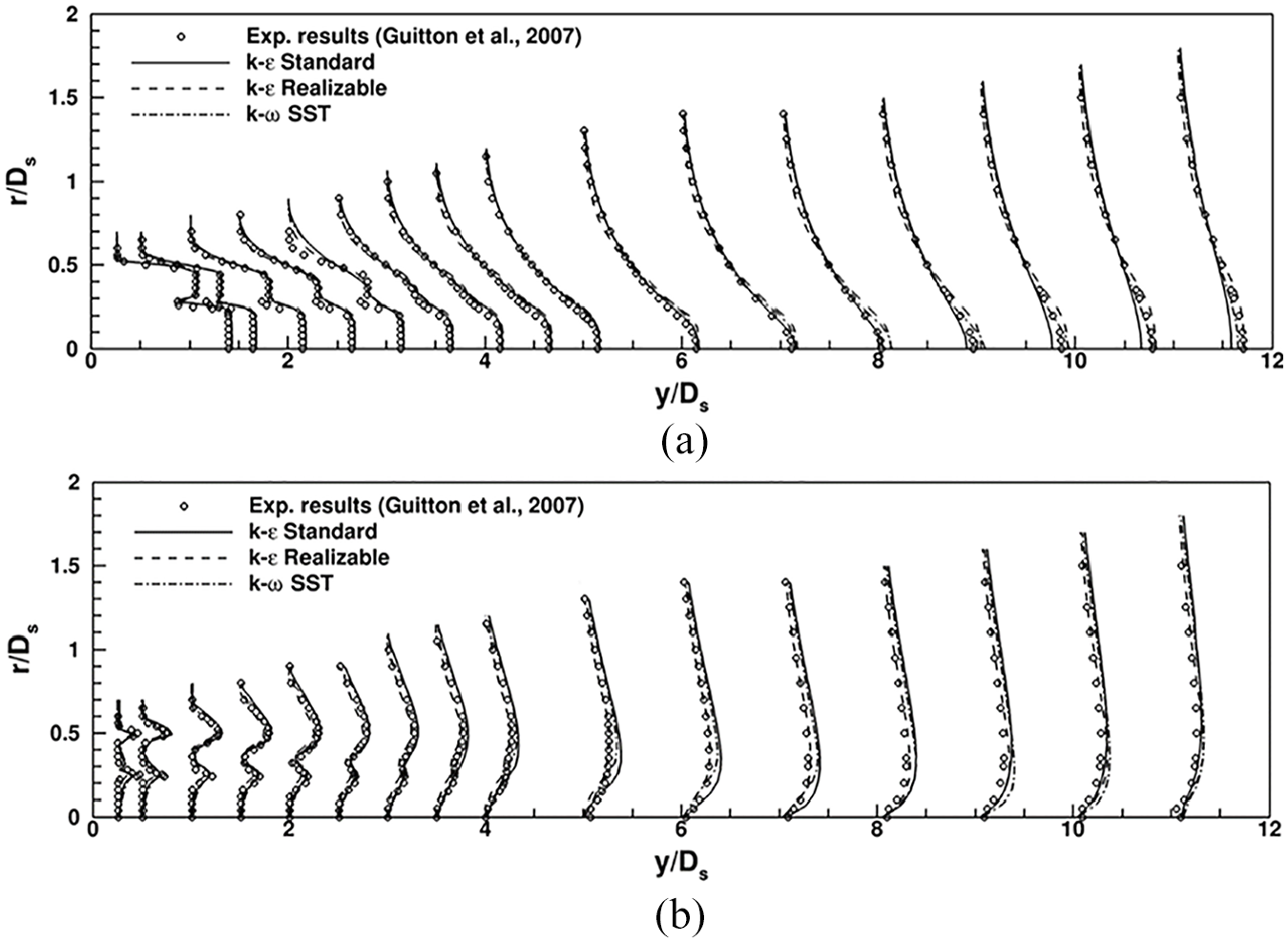
Comparison of exhaust-flow cross-sectional profiles for the three turbulence models tested against experimental results 31 : (a) axial velocity and (b) Reynolds stress.
To better assess the discrepancies observed near the jet axis in Figure 5(a), the performance study on turbulence models was carried out along the primary-jet centerline (see the results in Figure 6). The three models tested yielded similar performance in the potential core region (Figure 6(a)). In contrast, both velocity decay and TKE increase (Figure 6(b)) were best captured by the
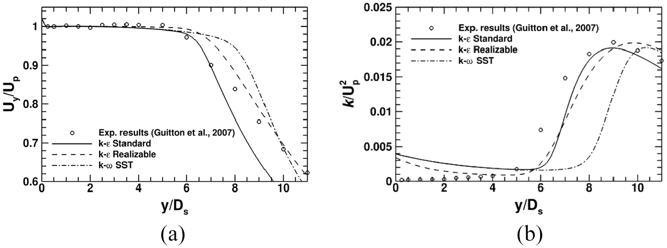
Comparison of primary-jet flow results for the three turbulence models tested against experimental results 31 : (a) axial velocity and (b) turbulent kinetic energy.
Contrail formation in the CFM56-3 exhaust jet
Computational domain and grid
Ice-particle formation was modeled in the exhaust plume of the CFM56-3 engine at realistic cruise flight conditions that ensure contrail formation.
27
The engine speed was set at
As the mean flow was assumed to be axisymmetric, only the 90° sector based on the engine nozzle was considered for URANS calculations, as shown in Figure 7. The geometry of the CFM56-3 short-cowl nozzle is composed of a core and a bypass flow whose diameters are
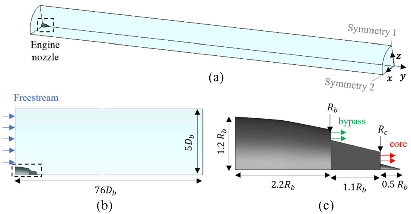
Computational domain and boundary conditions for the CFM56-3, short-cowl nozzle: (a) isometric view, (b) 2D view, and (c) nozzle geometry.
Exhaust conditions of the CFM56-3 engine. 53
As shown in Figure 7, the computational domain had a radius
The geometry and mesh of the computational domain were generated with ANSYS ICEM CFD software.
54
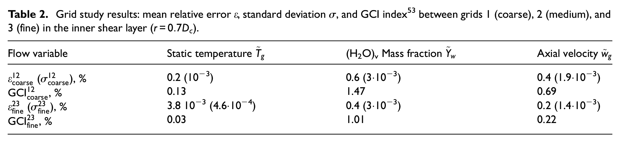
A grid convergence study was performed on the gaseous phase using three grids: coarse (4.35M cells), medium (9.8M cells), and fine (20.9M cells), respectively labeled grid 1, 2, and 3. The mean errors computed in the inner shear layer (i.e. between the core and the bypass jets) for the static temperature, water-vapor mass fraction, and core axial velocity are below 1% (see Table 2). Furthermore, discretization errors estimated using the GCI method
49
at a probe point (
Grid study results: mean relative error
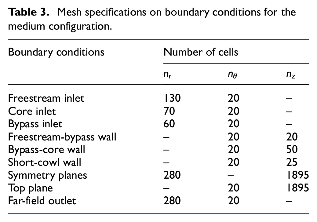
The medium grid is mainly composed of hexahedral elements, as shown in Figure 8. Three cell numbers
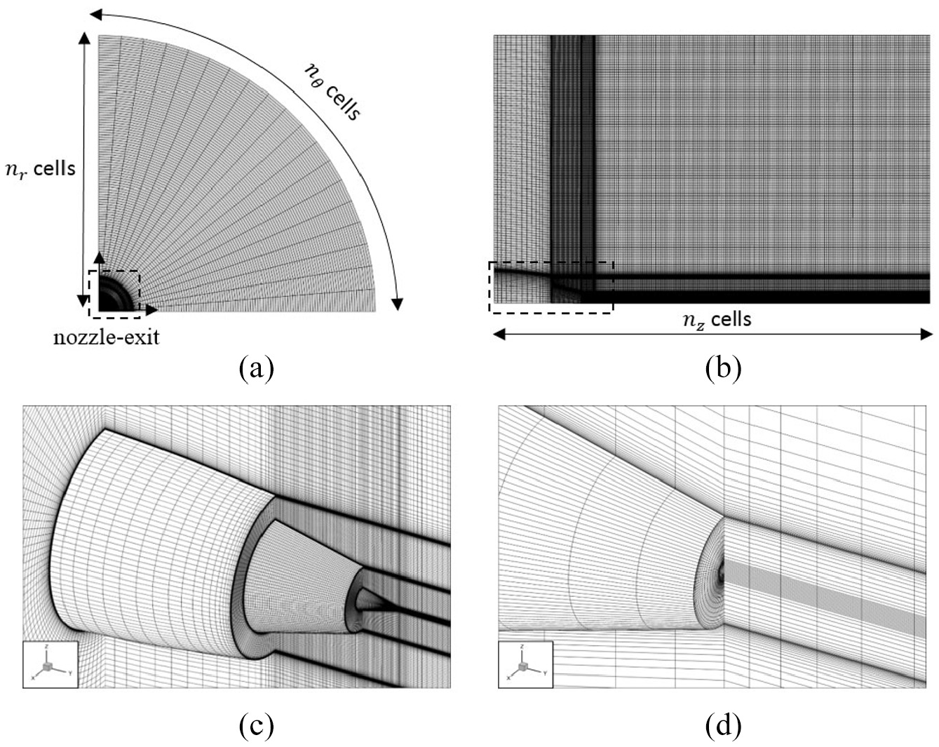
Computational grid for the medium mesh: (a) axial view, (b) lateral view, (c) close-up view of the nozzle exit, and (d) close-up view of the central plug.
Mesh specifications on boundary conditions for the medium configuration.
Jet flow and plume dilution
Figure 9(a) and (b) present the stream-wise contours of the axial mean velocity and Mach number, respectively, for the CFM56-3 plume. Since both dual-stream jets were at sonic conditions (M = 1), weak shock waves were observed near the exhaust sections and edges (Figure 9(b)); similar behavior was reported at nozzle-exit flows.55,56 A flow separation on the central plug can be seen in the core flow due to the over-expansion shock. The velocity contours in Figure 9(a) show that the potential core length was about
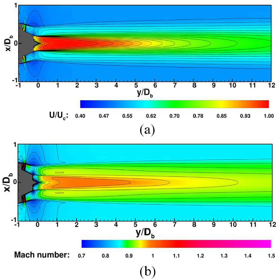
Stream-wise (xy-plane) contours of: (a) axial mean velocity and (b) Mach number.
The dilution ratio defined by Schumann et al. 58 was used to characterize the evolution of flow variables (such as temperature and contrail diameter) along the exhaust plume. The dilution ratio based on a passive scalar Z was calculated as
where
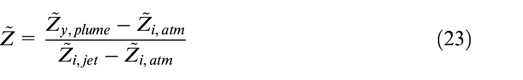
where
Figure 10 shows the evolution of the dilution ratio
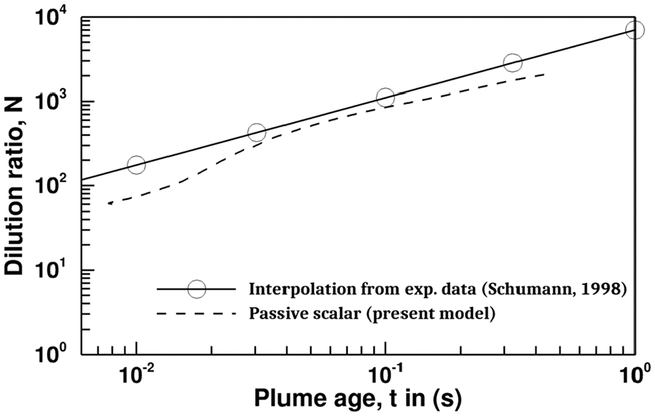
Evolution of the predicted dilution ratio along the primary jet centerline against in-flight measurements. 56
Contrail formation and ice-particle properties
Figure 11(a) presents the spatial distribution of ice-particle radii in the plume exhaust. Up to a distance of 10
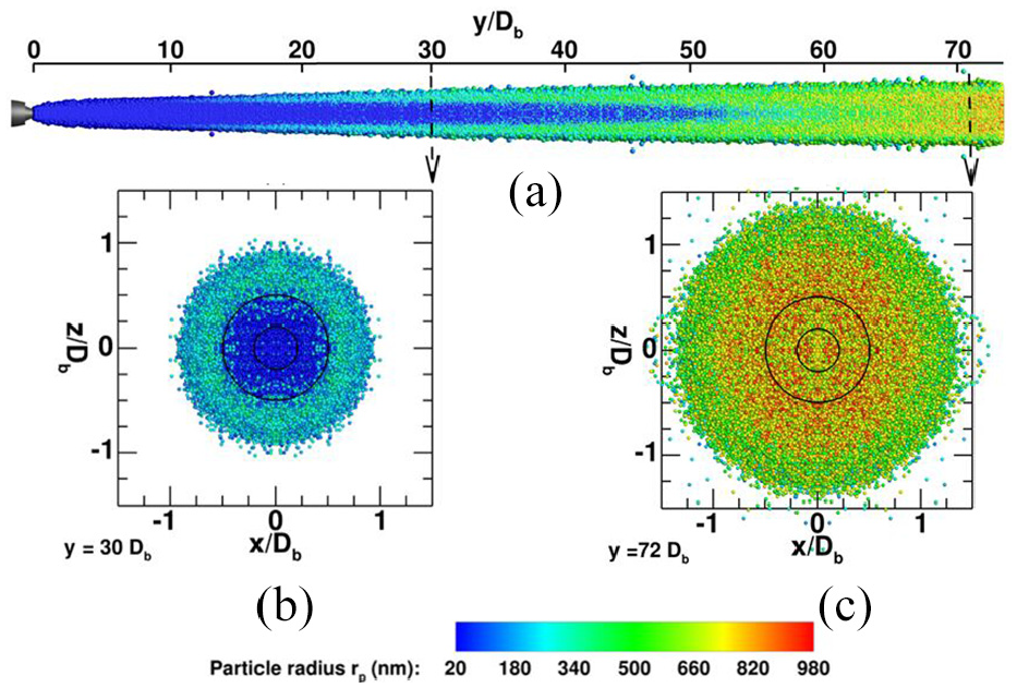
Spatial distribution of particle radii: (a) longitudinal cross-sectional distribution, transverse cross-sectional distributions at (b)
The rate of condensation along the exhaust plume was fully determined by the local ice saturation ratio S, which, in turn, depends on the local temperature
The evolution of the saturation ratio along the exhaust jet shows that the plume was fully saturated, that is,
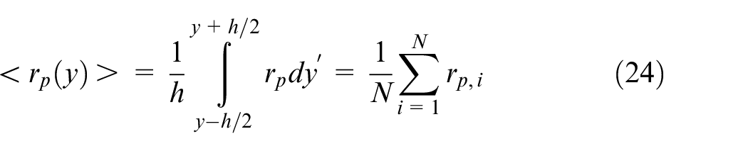
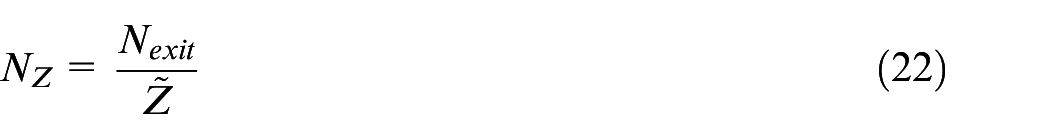
where N is the particle number within the considered subdomain and
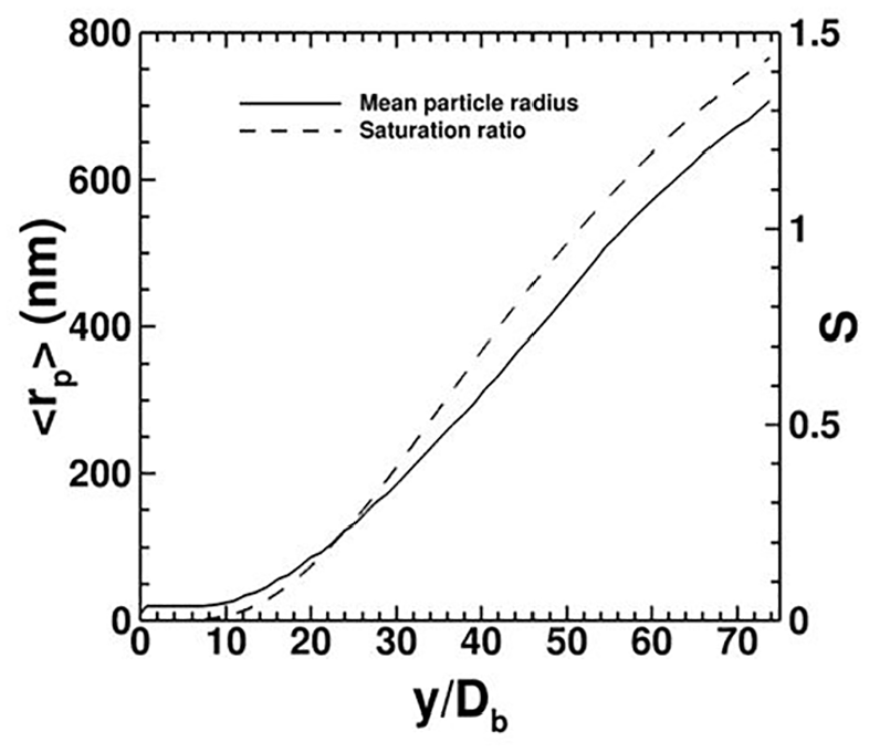
Evolutions of the mean particle radius and the saturation ratio along the jet plume.
To better assess the particle-size distribution along the exhaust plume, the probability density functions (PDF) were investigated at four distances:
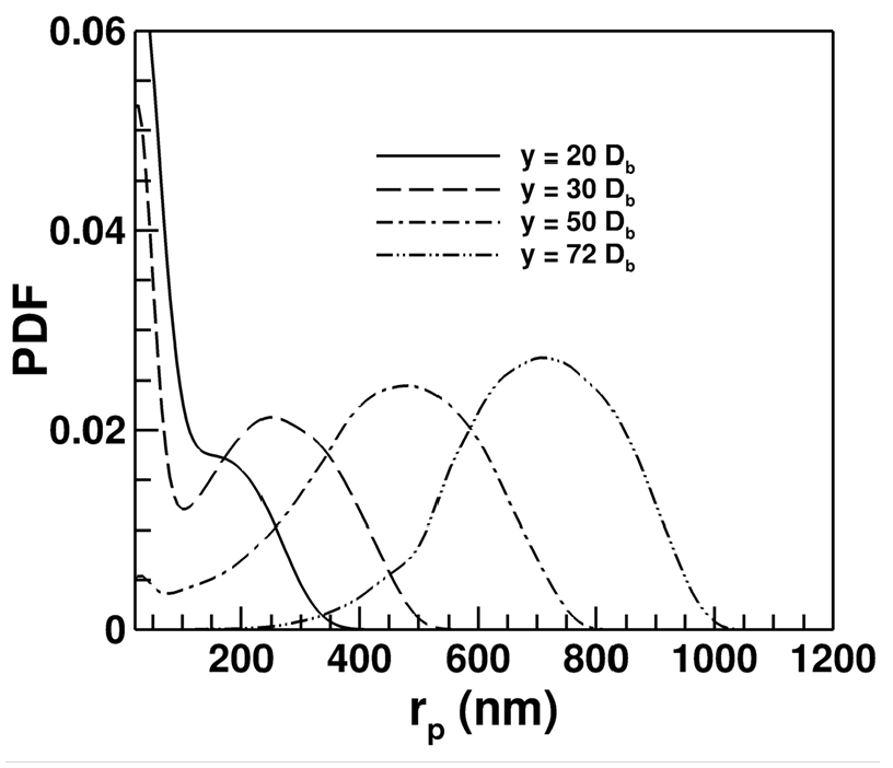
Probability density functions (PDF) of particle radius at four axial distances:
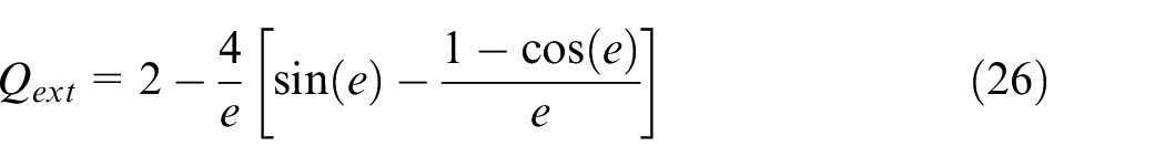
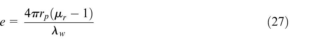
Lastly, the visibility in the predicted contrail was assessed with the optical depth
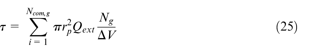
where
The visibility threshold of jet contrails is defined by the criterion
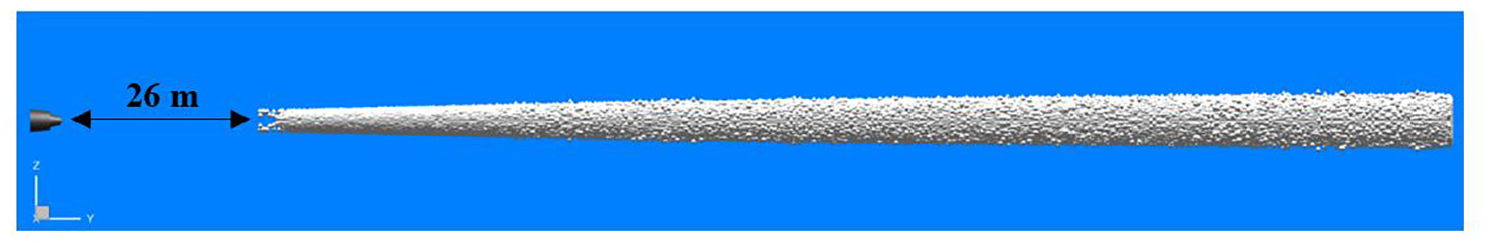
Visible contrail predicted in the near-field of the CFM56-3 engine using the visibility criterion
The comprehensive analysis performed shows that this model’s predictions are consistent with available numerical data. Such model can be used in future investigations to characterize the impact of complex nozzle geometries – such as chevron nozzles – on the optical and microphysical properties of near-field contrails. Research perspectives to be explored next involve the interactions of soot and sulfur species in the early plume. This requires the implementation of a gas-phase chemistry with the microphysics of volatile particles.
Conclusion
This paper demonstrated the feasibility of Eulerian–Lagrangian CFD coupling with ice microphysics to predict the near-field contrails starting from the nozzle-exit geometry of the CFM56-3 engine. The microphysical module implemented accounts for the main process of ice-particle growth based on heterogeneous nucleation. Two validation tests were performed to assess the reliability of the proposed CFD-microphysics model. In the first validation, the canonical case of compressible coaxial jets made it possible to choose the Realizable
The model presented herein is intended to serve as the foundation for more advanced numerical simulations to investigate the impact of complex nozzle-exit geometries, such as chevron nozzles. The implementation of gas-phase chemistry and volatile-particle microphysics are planned to extend the model capabilities.
Footnotes
Appendix A: Equations for the microphysical module
This appendix begins with a description of the factors
The factor
where
The conductivity of the gas was calculated from 64 :
The factor
where
The factor
where
The factor A in equations (19) and (20) was calculated as:
where
The diffusivity of water vapor was calculated from 64 :
The factor
where
The thermodynamic equation of the model is described. These equations depend on the particle temperature. The model considered the state of water. When the water was liquid (
The density of liquid water (kg·m−3) was calculated from 64 :
The surface tension of liquid water (J·m−2) was calculated from 66 :
The condensation latent heat of liquid water (J·kg−1) was calculated from 64 :
The saturation pressure of liquid water (Pa) was calculated from 67 :
The density of ice was (kg·m−3) calculated from 64 :
The surface tension of ice (J·m−2) was calculated from 66 :
The sublimation latent heat of liquid water (J·kg−1) was calculated from 64 :
The saturation pressure of ice (Pa) was calculated from:
Appendix B: Discretization of the ice particle growth equation
This appendix describe the discretization of ice particle growth equation (20) with a fourth order Runge-Kutta method. The four constants
The factor
where
The new particle radius
Then, the condensed matter of ice particles associated to equation (19) is calculated as follows
where n is the number density of particles contained in a volume cell V, such that
Acknowledgements
The authors thank Charles E. Tinney for providing data measurements on coaxial jets conducted at the Laboratoire d’Etudes Aérodynamiques (LEA) in Poitiers, France. Computations were made on the Beluga supercomputer at the École de technologie supérieure (ÉTS) in Montréal, managed by Calcul Quebec and Compute Canada.
Declaration of conflicting interests
The author(s) declared no potential conflicts of interest with respect to the research, authorship, and/or publication of this article.
Funding
The author(s) disclosed receipt of the following financial support for the research, authorship, and/or publication of this article: The operation of this supercomputer is funded by the Canada Foundation for Innovation (CFI), the Ministère de l’Économie, de la science et de l’innovation du Québec (MESI), 531, and the Fonds de recherche du Québec-Nature et technologies (FRQ-NT). The authors would also like to acknowledge the financial support of Safran Aircraft Engine for this work. This work is part of the Safran Industrial Research Chair on the Development of Sustainable Aero-Propulsion Systems at ÉTS.