On the use of particle image velocimetry (PIV) data for the validation of Reynolds averaged Navier-Stokes (RANS) simulations during the intake process of a spark ignition direct injection (SIDI) engine

Abstract

Computational fluid dynamics (CFD) simulations of the in-cylinder flow field are widely used in the design of internal combustion engines (ICEs) and must be validated against experimental measurements to enable a robust predictive capability. Such validation is complicated by the presence of both large-scale cycle-to-cycle variations and small-scale turbulent fluctuations in experimental measurements of in-cylinder flow fields. Reynolds averaged Navier-Stokes (RANS) simulations provide overall flow structures with acceptable accuracy and affordable computational cost for widespread industrial applications. Due to the nature of averaging physical parameters in RANS, its validation against experimental results obtained by particle image velocimetry (PIV) requires consideration of how best to average or filter the measured turbulent flows. In this paper, PIV measurements on the cross-tumble plane were recorded every five crank angle degrees for $300$ cycles during the intake process of a motored, optically accessible spark ignition direct injection (SIDI) engine. Several methods including ensemble averaging, speed-based averaging and low-order proper orthogonal decomposition (POD) reconstruction were applied to remove the fluctuations from experimental PIV vector fields and thus enable comparison to RANS simulations. Quantitative comparison metrics were used to evaluate the performances of each method in representing the intake jet. Recommendations are made on how to provide a fair validation between measured data and simulation results in highly fluctuating flow fields such as the engine intake jet.

Introduction

Internal combustion engines (ICEs) continue to serve as the main source of power for ground transportation worldwide, as vehicles with an ICE (including both conventional ICE and hybrid vehicles) retained over $90$ % of the worldwide market share in $2018$ . ¹ Predictions show that the market share of battery electric vehicles (BEVs) may only reach 11%–28% by $2040$ , ² despite its rapid growth in recent years. Hybrid vehicles have been found to be a viable alternative to BEVs in terms of sustainability, ³ particularly when the life-cycle greenhouse gas emissions are considered.^4,5 The trend towards hybridisation continues to motivate the study of physical phenomena occurring within the engine cylinder, in order to design more efficient engines for future hybrid vehicles that can meet emission regulations and provide a cleaner environment.

The performance of spark ignition direct injection engines is strongly influenced by the complex in-cylinder air motion initiated by the intake process, as the air-fuel mixture is formed inside the engine cylinder. The homogeneity of the mixture relies greatly on the intake air speed, flow structure and turbulence level, and it further influences the combustion quality and the emissions from the engine. ⁶ The development of flow simulation models using computational fluid dynamics (CFD) tools such as the Reynolds averaged Navier-Stokes (RANS) and the large eddy simulation (LES) approaches^7–10 have been accelerating engine design and reducing the number of engine tests, yet the models still need to be validated by experimental measurements to provide more accurate predictions of the highly fluctuating and reacting flow. ¹¹ Both RANS and LES simulate the large structures of the in-cylinder flow, and LES provides an additional access to the cycle-to-cycle variation in the engine. ¹² However, the computational cost of LES is considerably higher than RANS, and therefore RANS is still widely used in industrial applications where the time for the engine research & development cycle is critical and limited.

Various flow velocity measurement techniques have been developed over the years, and the particle image velocimetry (PIV) technique has become the most widely used for engine in-cylinder flow research since it provides high spatial and high temporal resolution measurements of the rapidly-changing flow.^13,14 In engine research, PIV has been used to visualise a variety of in-cylinder flow behaviours – from the bulk air flow such as the intake-induced tumbling/swirling motions^15,16 and the flow-spray interactions, ¹⁷ to smaller-scale structures including the boundary layer near the cylinder head ¹⁸ and flow fields close to the spark plug. ¹⁹

Multiple studies have been focusing on the validation of in-cylinder flow fields modelled by RANS simulations.^20–24 As the RANS model only provides an averaged flow field at a certain engine phase (crank angle), the PIV measurements in multiple engine cycles need to be averaged into a single field in order to enable a comparison. One common approach is to use the phase-averaged ensemble mean (averaged flow field at fixed crank angle), assuming the engine operation is a cyclostationary process. ²⁵

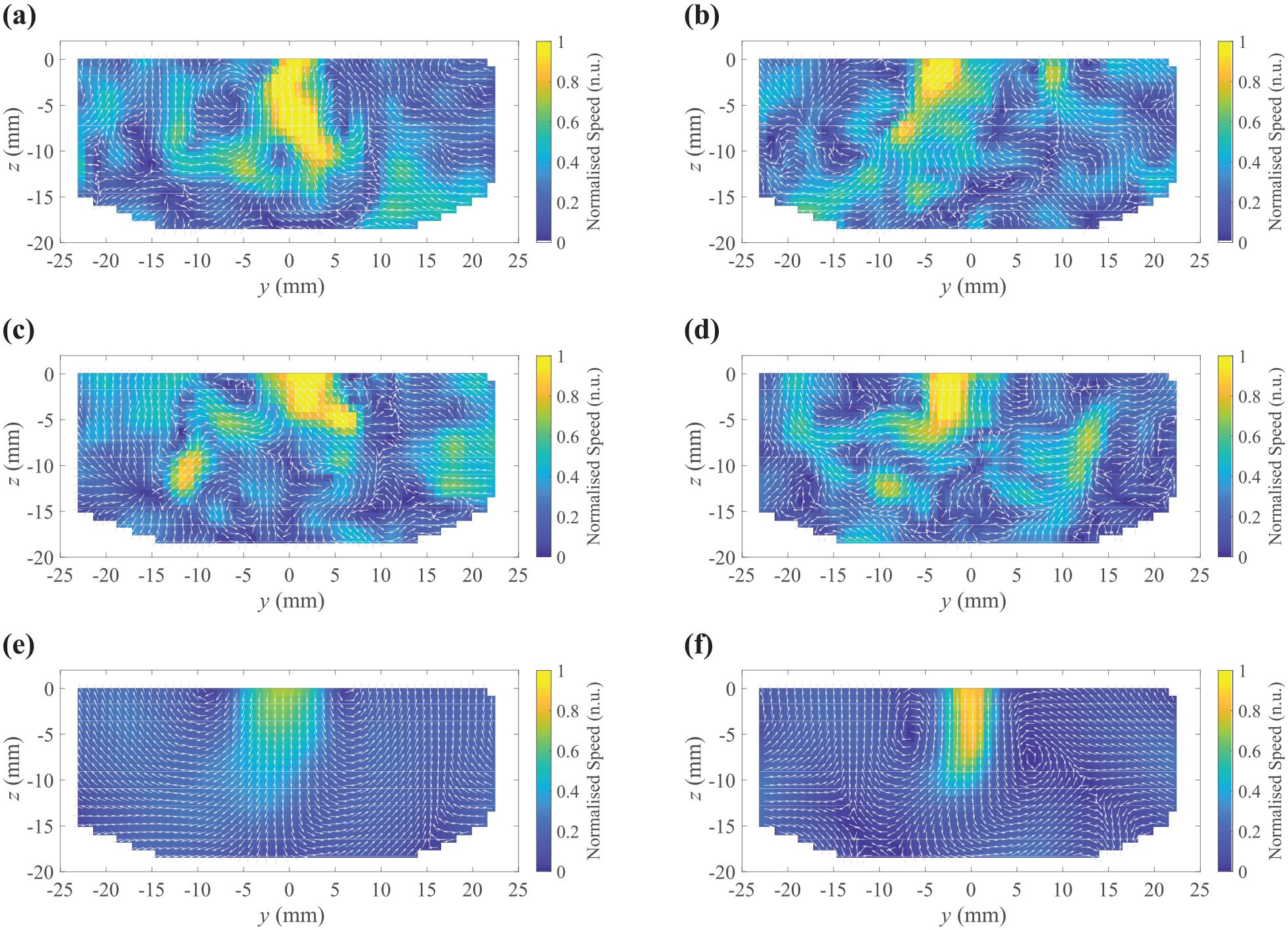
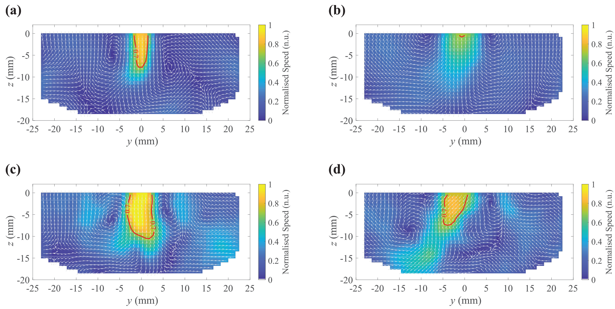
During the intake stroke, however, engine flow fields measured by the PIV technique show the flow to have high turbulence and cycle-to-cycle variations that include intake jet flapping. ²⁶ For instance, as illustrated in the PIV-measured intake flow for four different engine cycles (Figure 1(a)–(d)), the intake streams from both intake valves collide near the symmetric centreline plane of the engine ( $y=0$ ), resulting in a generally downward-moving central intake jet viewed from the intake side of the engine. Despite the engine being geometrically symmetric with respect to the central plane ( $y=0$ ), the two intake streams may have different strengths due to upstream fluctuations. As a result, the central intake jet observed on the plane swings from left to right (Figure 1(a)–(c)), or enters the field of view displaced to one side of the engine (Figure 1(a) vs (d)). The ensemble averaging of the experimental data (Figure 1(e)) smooths out the fields and cancels horizontal components of the flow, which causes the velocity magnitude of the averaged intake jet to be lower than that of the RANS simulation and those of individual cycles. Previous comparisons of RANS simulated data to PIV measurements in the tumble plane by the authors, ²³ via point-by-point vector comparison metrics for alignment and magnitude, noted similar results where RANS velocity magnitudes were higher than those of ensemble-averaged PIV data during the intake process. Therefore, if the ensemble mean is used to validate the RANS modelled flow field for fluctuating coherent structures (Figure 1(f)), the validation would be heavily skewed and may even result in a false conclusion.

Figure 1.

Flow fields at $300$ crank angle degrees (CAD) before the firing top dead centre (bTDCf): (a) PIV cycle A, (b) PIV cycle B, (c) PIV cycle C, (d) PIV cycle D, (e) PIV ensemble mean and (f) RANS simulation.

The mismatch between the averaged PIV flow fields and the RANS simulation comes from their fundamental differences in averaging mechanisms – the averaged PIV takes multiple measured vector fields and computes pure mathematical means of the vectors at each location to generate an artificial field (namely the ensemble mean), while RANS adopts averaged physical quantities from the PIV experiment into a physics-based model that is governed by averaged thermo-fluid equations. It is recognised that RANS simulations cannot capture the unsteady nature of practical flows, ²⁷ and the large-scale cycle-to-cycle flow variations presented in the in-cylinder PIV flow fields are not represented in the RANS equations of motion. All fluctuations are simulated by a statistical-closure model (such as the k- $ϵ$ model^28,29) in RANS for turbulence production and dissipation. An alternative method to the PIV ensemble mean is therefore required to filter the turbulence and cycle-to-cycle variation within the experimental flow fields, and to extract their major organised fluid motions (known as ‘coherent structures’) to enable a fair validation for the RANS flow predictions.

Proper orthogonal decomposition (POD), a variant of principle component analysis (PCA) originally proposed by Lumley, ³⁰ has been extensively used in recent research on IC engine in-cylinder velocity fields.^31–35 POD considers each of the velocity components measured at the same spatial location as a random variable and therefore treats the entire flow field as a multivariate data set. The result of POD is a series of ranked flow patterns (known as POD modes) which are computed by successively maximising the sample variance within the ensemble and equivalently, the total amount of kinetic energy distributed into each mode. Based on this successive kinetic energy maximisation property, the first several low order POD modes collectively account for the majority of the high energy flow features within the dataset, and therefore the combination of them is regarded as the coherent structure of the ensemble. The higher order POD modes, which are discarded due to their small kinetic energy fractions, are often associated with random Gaussian fluctuations, ³² smaller-scale turbulence^34,36 or measurement noise.^37,38 As such, it is possible to implement POD as a dimension reduction technique to reduce the flow complexity and as a low-order approximation tool to extract the dominant structure of the in-cylinder turbulent flow measured in each cycle (at the same crank angle), and use the POD-reconstructed/approximated flow fields to validate the simulation results. It should be noted that POD is chosen in this application over other filtering methods such as spatial filtering by convolution with a Gaussian kernel or application of a cut-off spatial frequency, ³⁹ since POD is capable of extracting coherent flow structures without losing spatial resolution in the filtered fields. A high spatial resolution is critical to the determination of the region which the intake jet occupies, and the jet region is of interest in this paper.

Once the coherent structures of the flow fields from individual cycles have been extracted, comparison to RANS requires quantification of the intake jet characteristics. Point-by-point comparison metrics for vector fields, such as those developed previously by the authors to compare RANS simulated data to PIV measurements in the tumble plane,^23,24 can quantify the similarity of pairs of fields and identify regions of interest. However, point-wise comparisons cannot account for similarities between fields which arise from the displacement or distortion of coherent structures. In the individual flow fields of this work, the intake jet typically maintains a coherent structure but shows significant cycle-to-cycle variation in its shape, direction and location (Figure 1(a)–(d)). Therefore rather than a point-wise comparison, quantities such as the intake jet angle, penetration length and width are defined and evaluated for each flow field. The values of these jet quantification metrics for the RANS simulation are compared to the range of experimental PIV results in order to provide a representative validation target for the RANS simulation.

In the later sections of this paper, the PIV experiment details for measuring crank angle-resolved flow fields in a single cylinder version of a near-production engine are first presented, followed by the numerical setup for the RANS model that simulates the in-cylinder flow based on the boundary conditions measured during the PIV experiment. A set of metrics is then developed to quantify the intake jet profile; several other existing flow comparison metrics as well as the notations and properties of POD are also summarised. The RANS simulated flow at a specific crank angle during the intake stroke is chosen to exemplify its validation process against averaged or filtered PIV data that were computed using different approaches. Various methods are tested, including the phase-averaged ensemble mean, the modified mean flow field based on a speed average, and the individual cycles approximated by the low-order POD reconstruction, among which the low-order POD reconstructed flow fields give a fairer and more robust comparison with the simulated data. During the process, a stability test is also developed to determine the number of modes needed in the low-order POD reconstruction.

Data acquisition apparatus and methods

Optically accessible engine and particle image velocimetry

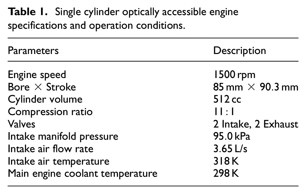
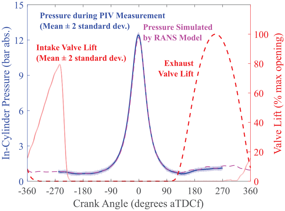
The experimental data were obtained in a single-cylinder spark ignition direct injection (SIDI) optically accessible engine based on an existing production engine (Ingenium, Jaguar Land Rover), whose specifications and operation conditions are listed in Table 1. A pressure transducer (Kistler $6043$ A $60$ ) installed on the pent roof recorded crank angle-resolved in-cylinder pressure (blue solid line with shaded error bar of two standard deviations about the mean in Figure 2) for each cycle. The real-time intake valve lift (red solid line also with shaded error bar in Figure 2) was measured using a Sensitec valve train measurement system (VTMS.DSE. $02$ ) through machined grooves on the inlet valve stems. A continuously variable valve lift (CVVL) system installed between the intake camshaft and valves enables delayed inlet valve opening and/or early intake valve closing. The exhaust valves are connected to the camshaft by roller finger followers (RFF), and the exhaust valve lift (red dashed line in Figure 2) was calculated by the known valve profile and its maximum opening point. The cylinder liner is divided into two parts: the upper part is a quartz annulus (height varies from $25$ to $39$  mm) which gives optical access; the lower part is a metal barrel with internal water cooling in order to provide additional cooling to the Torlon piston rings. The engine was operated under motored (no fuel injection, no ignition) conditions.

Table 1.

Single cylinder optically accessible engine specifications and operation conditions.

Parameters	Description
Engine speed	$1500$  rpm
Bore × Stroke	$85$  mm ×  $90.3$  mm
Cylinder volume	$512$  cc
Compression ratio	$11:1$
Valves	$2$ Intake, $2$ Exhaust
Intake manifold pressure	$95.0$  kPa
Intake air flow rate	$3.65$  L/s
Intake air temperature	$318$  K
Main engine coolant temperature	$298$  K

Figure 2.

Engine operation parameters.

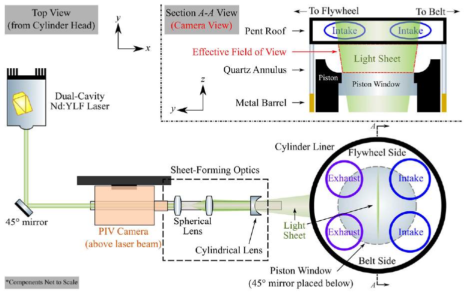
A planar particle image velocimetry technique^40,41 was applied to measure two-dimension/two-component (2D/2C) flow fields inside the engine cylinder. Figure 3 illustrates the PIV experimental setup. A diode-pumped, dual-cavity Nd:YLF laser (Photonics Industries DM $20$ - $527$ -DH) provided a pulsed output beam of approximately $17$  mJ per pulse at a repetition rate of $1.8$  kHz (for each cavity) at $527$  nm. The beam was aligned to the central axis of the engine cylinder, before forming the desired light sheet using a set of optics: a spherical lens telescope relay reduced the beam diameter and compensated for its natural divergence, and a negative cylindrical lens expanded the beam in one direction and generated the light sheet. A ${45}^{°}$ mirror was placed beneath the piston window within the hollow Bowditch ⁴² extension using a sliding rail mount for ease of installation and cleaning of the quartz annulus. The light sheet was thus directed towards the cylinder head, travelled through the quartz piston window ( $46$  mm diameter) and illuminated the central cross-tumble plane. (The plane separates the pair of intake valves from the pair of exhaust valves; denote Section A-A in Figure 3) A high-speed CMOS camera (Vision Research Phantom VEO $710$ L) was used to record the scattered light from the seeding oil droplets ( $0.2-0.4$  μm in diameter), which were introduced by mixing with air in a plenum upstream of the intake runner to ensure a uniform distribution. The resulting effective field of view (the camera view in Figure 3) spans from the cylinder head fire deck to the face of the piston crown (when the piston is closer to TDC), or to the bottom edge of the quartz annulus (when the piston position is lower).

Figure 3.

PIV setup for cross-tumble plane flow measurement.

The laser and camera were synchronised by a programmable timing unit (LaVision PTU X) with a frame straddling approach.^43,44 The two images that were used to generate one vector field were illuminated respectively by laser pulses from each of the laser cavities. The time separations between the two pulses (often termed as ‘d $t$ ’) were optimised based on the varying in-cylinder velocities; the maximum particle displacement was limited to eight pixels ( $25$ % of the final interrogation window size) to improve the calculation accuracy. ⁴⁵

The pairs of images were recorded every five crank angle degrees (CAD) from $330$ to $30$  CAD bTDCf (before the firing top dead centre). Three experimental runs each of $100$ consecutive cycles were performed to build a $300$ -cycle dataset. Raw images were processed in the DaVis^® software (LaVision, Ver. $8.4.0$ ) to generate vectors. Two pre-processing functions were applied: the background subtraction (Gaussian sliding average over cycles) removes the light reflections from the metal surfaces in the cylinder; the particle intensity normalisation compensates for variations in intensity between individual droplet images across the field of view. The multi-pass algorithm reduced the interrogation window from $128\times 128$ -pixels to $32\times 32$ -pixels with $50$ % overlap,^46,47 to evaluate the PIV vectors, resulting in a vector spacing of $0.84$  mm. Local spurious vectors whose peak ratios (corresponding to the ratio of correlation values between the highest and the second highest correlation peaks ⁴⁸ ) smaller than two were removed from the final vector fields, and these removed vectors were not replaced by any interpolation methods. The total number of removed vectors was less than $0.1$ %.

Reynolds averaged Navier-Stokes simulation

The in-cylinder flow fields were simulated by Siemens STAR-CD^® software with the es-ice™ package (ver. $4.26.022$ ) using the k- $ϵ$ RNG turbulence model.^28,29 The time step was set to $0.1$ CAD (or 11.1 μs at $1500$ rpm engine speed), with refinements of $0.05$ CAD close to the valve opening and closing, as well as during valve overlap. The automatically trimmed mesh generated over $3.3$ million cells with $0.7$  mm mesh size. The mesh was refined to $0.3$  mm both upstream and downstream of the intake valves when the valves are open, in order to accurately model the intake process.

The RANS simulation used the same engine geometry as the optical engine, and was initialised before the exhaust valve opening, that is, in a closed control volume, during the late expansion stroke. The following parameters measured during experiments were used as boundary conditions:

1. phase-averaged crank angle-resolved intake and exhaust valve lifts,

2. phase-averaged crank angle-resolved pressures inside the inlet and exhaust runners (measured by Kistler $4075$ A $10$ transducers),

3. time-averaged intake, exhaust and main engine coolant temperatures,

4. time-averaged intake air volume flow rate.

Due to the unknown amount of blow-by during the optical engine operation, the piston crevice length was tuned in the model in order to match the in-cylinder pressure traces with the experiments. There were no other physical parameters adjusted during the simulation. The difference of in-cylinder pressure between the experiment ( $300$ -cycle average, blue solid line in Figure 2) and the simulation (purple dashed line in Figure 2) was less than $1.8$ % at all crank angles.

Data analysis approaches

Quantification of intake jet profile

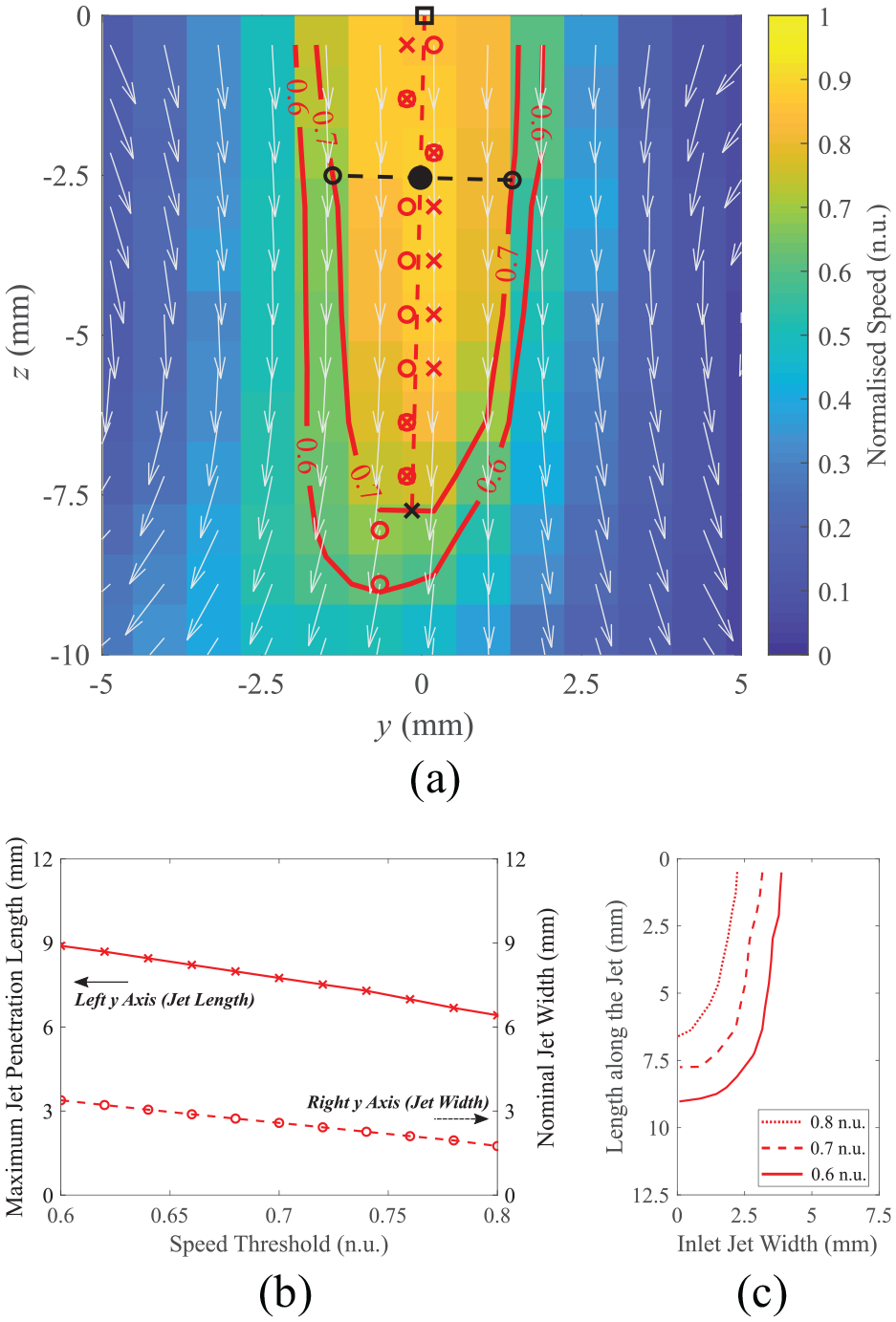
As mentioned in the introduction, the intake jet can vary significantly from cycle to cycle. Therefore, this section aims to develop metrics to quantify the intake jet profile, and seeks to provide a tool to compare two vector fields that contain the intake jet. A zoomed-in plot for the RANS simulated flow field at $300$ CAD bTDCf (Figure 1(f)) is presented in Figure 4(a) near the intake jet region. The flow speed is normalised by a speed specified by Jaguar Land Rover’s protocol, and thus all the flow speed are in normalised units (denoted by ‘n.u.’). The following procedures were proposed to find the jet angle, the jet penetration length and the nominal jet width.

Figure 4.

Intake jet profile definitions illustrated by a RANS simulated flow field at $300$  CAD bTDCf: (a) intake jet regions at $0.6$  n.u. and $0.7$  n.u. speed thresholds. Red hollow circles: centre points at $0.6$  n.u. speed threshold; Red crosses: centre points at $0.7$  n.u. speed threshold; Red dashed line: fitted jet centreline; Black hollow square: jet entry point on the centreline; Black cross: jet end point on the centreline at $0.7$  n.u. speed threshold; Black filled dot: an example point on the centreline; Black dashed line: line perpendicular to the centreline and passes through the example point; Black hollow circles: intersections of the perpendicular line and the jet region boundary at $0.7$ n.u. speed threshold, (b) left $y$ axis: jet penetration length (red solid line with crosses) as a function of the speed threshold; Right $y$ axis: nominal jet width (red dashed line with hollow circles) as a function of the speed threshold, (c) intake jet profiles (width as a function of length) at $0.8$  n.u. (dotted line), $0.7$  n.u. (dashed line) and $0.6$  n.u. (solid line) speed thresholds.

Jet Angle

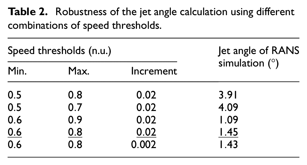
The high-speed intake jet and low-speed background were first identified by choosing appropriate speed thresholds. For instance, the red contour lines in Figure 4(a) illustrate the jet profile using $0.6$ and $0.7$  n.u. speed thresholds, respectively. The jet region is therefore bounded by the top edge of the PIV field of view ( $z=0$ , at the fire-deck) and the jet profile at the given speed threshold. For each speed threshold, the centre points on each row (constant $z$ values) of its jet region were then obtained (e.g. red hollow circles for $0.6$  n.u. and red crosses for $0.7$  n.u. in Figure 4(a)). In order to have a unique and robust jet centreline (red dashed line) for a given flow field, the centre points were found for a sequence of threshold values as defined in Table 2, in terms of the range of the threshold values and their increment. The centreline of the jet was defined by performing a linear fit to all the centre points, no matter whether or not they were obtained using the same speed threshold (i.e. consider the red hollow circles and red crosses as equivalent). This approach puts more weight on the higher-speed regions since there are more points taken into account, and thus avoids the jet centreline being skewed towards the tip of the jet, whose direction fluctuates drastically among the low speed thresholds. The angle between the jet centreline and the jet propagation direction (in this case the $z$ axis) is the jet angle. A robustness check (Table 2) for the jet angle of a RANS simulated flow field (Figure 4(a)) shows that the evaluated jet angle is stable within a few degrees for different combinations of speed thresholds. All the jet angles presented in later parts were obtained by using the speed threshold combination which has a minimum speed threshold of $0.6$  n.u., at $0.02$  n.u. increment, to a maximum of $0.8$  n.u. (highlighted using underlines in Table 2). All these speed thresholds will be used to evaluate the jet penetration lengths and nominal jet widths for any given flow field, in order to provide an overall comparison of jet profiles between the experimental and simulated data.

Table 2.

Robustness of the jet angle calculation using different combinations of speed thresholds.

Speed thresholds (n.u.)			Jet angle of RANS simulation (°)
Min.	Max.	Increment
$0.5$	$0.8$	$0.02$	$3.91$
$0.5$	$0.7$	$0.02$	$4.09$
$0.6$	$0.9$	$0.02$	$1.09$
$\underset{¯}{0.6}$	$\underset{¯}{0.8}$	$\underset{¯}{0.02}$	$\underset{¯}{1.45}$
$0.6$	$0.8$	$0.002$	$1.43$

Jet penetration length

Once the jet centreline is determined, the jet penetration length for each flow field can be found by calculating the largest distance among its intersections with the jet region at a certain speed threshold. For instance, the distance between the black cross and the black hollow square in Figure 4(a) gives a jet penetration length of $7.7$  mm at the $0.7$  n.u. threshold. The jet penetration length decreases at higher speed thresholds (red solid line with crosses in Figure 4(b)). The slope of the line also shows the velocity gradient along the jet propagation direction – a more negative (steeper) slope means the velocity gradient is smaller, since the distance between two constant speed lines is larger.

Nominal jet width

Given an arbitrary point on the jet centreline inside the jet region (black solid dot in Figure 4(a)), a unique line (black dashed line) can be drawn that passes through the point and perpendicular to the jet centreline. When this perpendicular line intersects with the contour of each given speed threshold at two point locations (black hollow circles for $0.7$  n.u. in Figure 4(a)) on opposite sides of the jet centreline, the jet width corresponding to that point on the centreline is defined as the distance between these two intersections. If there is only one intersection detected (occurs when the arbitrary point on the jet centreline is too close to the entry of the jet), the jet width for that arbitrary point is not defined. Figure 4(c) illustrates the jet width as a function of length along the jet (distance away from the jet entry, black hollow square in Figure 4(a)) at three different speed thresholds. Due to the convergent shape, the jet width generally decreases from the entry (top) to the tip of the jet (bottom). The jet is wider for lower speed thresholds for the same jet length, which can also be intuitively observed in Figure 4(a). In order to have a single quantity for the jet width, the median of the jet width at all lengths along the jet for a certain speed threshold is selected to be the nominal jet width, which is also larger at the lower speed threshold (red dashed line with hollow circles in Figure 4(b)). The median was chosen against the mean to provide a more robust result that would otherwise be skewed by the highly-curved jet tip. The slope of the nominal jet width versus speed thresholds also illustrates the velocity gradient perpendicular to the jet propagation direction – again, a more negative (steeper) slope leads to a smaller velocity gradient.

Relevance index

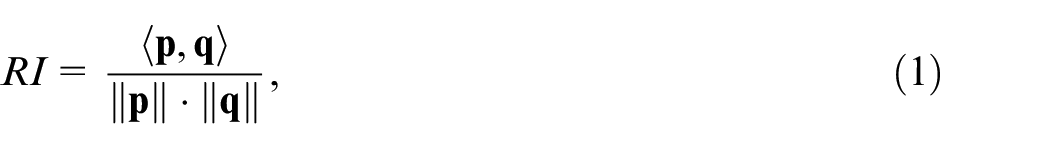
In addition to the jet profile, the overall flow structure on the cross-tumble plane is of interest as well. This requires metrics that can quantify the directional similarity between two vector fields. Liu and Haworth ⁴⁹ used the normalised scalar product of the two vector fields, and termed it the relevance index ( $\mathrm{RI}$ ):

$$\mathrm{RI}=\frac{〈\mathbf{p},\mathbf{q}〉}{\Vert \mathbf{p}\Vert ·\Vert \mathbf{q}\Vert },$$

(1)

where $〈\mathbf{p},\mathbf{q}〉$ is the inner product of vector fields $\mathbf{p}$ and $\mathbf{q}$ , ‖·‖ represents the ${\mathbb{L}}^2$ norm; each vector field is re-arranged to a column vector with many ( $2\times$ grid points) components in the calculation. The value of $\mathrm{RI}$ ranges from $-1$ to $+1$ , in which $+1$ means the two vector fields are in perfect alignment.

By first re-arranging the vector fields $\mathbf{p}$ and $\mathbf{q}$ into column vectors, this application of the relevance index returns a single scalar value for the whole-field comparison of two vector fields. If the spatial variation in local ‘quality of alignment’ across the field is of interest, an alternative approach is to perform a point-by-point comparison by calculating the $\mathrm{RI}$ value separately at each spatial coordinate, returning a spatially-resolved ‘alignment quality’ field result ⁵⁰ (equivalent to the Local Structure Index, $\mathrm{LSI}$ ⁵¹ ). At each coordinate, the input vectors for equation (1) would be the individual vectors at the corresponding location within each field. This point-wise method is highly sensitive to misalignment in regions of small vector magnitudes, where small absolute differences result in large differences in vector direction. To enable a point-wise comparison which is sensitive to the alignment of both large and small vector magnitudes, previous work by the authors introduced weightings based on the local vector magnitude compared to the flow field as a whole: the Weighted Relevance Index ( $\mathrm{WRI}$ ), Weighted Magnitude Index ( $\mathrm{WMI}$ ) and Combined Magnitude and Relevance Index ( $\mathrm{CMRI}$ ).^23,24 In this work a spatially-resolved ‘alignment quality’ field result is not required, only an overall ‘whole-field’ comparison of whether the POD approximations have reached a converged result. Therefore, the whole-field application of the $\mathrm{RI}$ ⁴⁹ (equation (1)) was used for conciseness and to avoid the introduction of alternative metrics ( $\mathrm{WRI}$ , $\mathrm{WMI}$ , $\mathrm{CMRI}$ ) which require velocity weighting and spatial averaging only to arrive at a comparable whole-field result.

Flow field averaging metrics

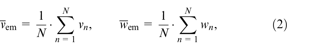
In this section, two metrics that were used to average the PIV flow fields are defined to facilitate later discussion. Given a set of PIV flow fields $\{{\mathbf{V}}_n=(v_n,w_n)\}$ that were measured at the same crank angle in different cycles ( $n=1,2,\cdots ,N$ ), the phase-averaged ensemble mean ${\overline{\mathbf{V}}}_{\mathrm{em}}=({\overline{v}}_{\mathrm{em}},{\overline{w}}_{\mathrm{em}})$ can be found by:

$${\overline{v}}_{\mathrm{em}}=\frac{1}{N}·\sum _{n=1}^N{v}_n,{\overline{w}}_{\mathrm{em}}=\frac{1}{N}·\sum _{n=1}^N{w}_n,$$

(2)

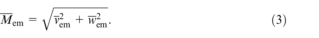
where the subscript em denotes ensemble mean, $v_n$ and $w_n$ are, respectively, the velocity components along the horizontal ( $y$ ) and vertical ( $z$ ) axes for Cycle $n$ . The magnitude (speed) of the ensemble mean, which was plotted as the colour map in Figure 1(e), is calculated by:

$${\overline{M}}_{\mathrm{em}}=\sqrt{{\overline{v}}_{\mathrm{em}}^2+{\overline{w}}_{\mathrm{em}}^2}.$$

(3)

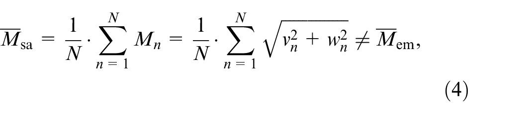
Note that equation (3) is different from the mean of the magnitude (average of speed) for all cycles:

$${\overline{M}}_{\mathrm{sa}}=\frac{1}{N}·\sum _{n=1}^N{M}_n=\frac{1}{N}·\sum _{n=1}^N\sqrt{v_n^2+w_n^2}\ne {\overline{M}}_{\mathrm{em}},$$

(4)

where the subscript sa denotes speed average. The magnitudes of each cycle $M_n$ were plotted as the colour map for Figure 1(a) to (d).

Proper orthogonal decomposition

As discussed in the introduction, proper orthogonal decomposition offers a statistical way to analyse turbulent flow data. In this section, the notations and several properties of POD are presented. Following the Reynolds decomposition approach, ⁵² the phase-averaged ensemble mean is first subtracted from each flow field, leaving the fluctuation velocity field ${\mathbf{V}}_n^{\prime }$ :

$${\mathbf{V}}_n^{\prime }={\mathbf{V}}_n-{\overline{\mathbf{V}}}_{\mathrm{em}}.$$

(5)

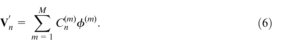
The proper orthogonal decomposition^53–55 to the set of $\left\{{\mathbf{V}}_n^{\prime }\right\}$ separates the fluctuation flow fields (again, obtained from different cycles at the same engine phase) into a linear combination of POD modes, denoted by ${\varphi }^{(m)}$ ( $m=1,2,\cdots ,M$ ):

$${\mathbf{V}}_n^{\prime }=\sum _{m=1}^M{C}_n^{(m)}{\varphi }^{(m)}.$$

(6)

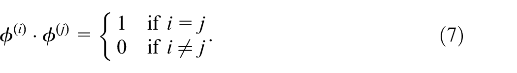
All the cycles share the same set of POD modes, while their coefficients $C_n^{(m)}$ differ from cycle to cycle for a single mode, and vary among different POD modes for a single cycle. Each term $C_n^{(m)}{\varphi }^{(m)}$ can be regarded as one component of the original field. The POD modes are normalised fields and serve as the basis of the set of flow fields. POD modes are orthonormal, that is,

$${\varphi }^{(i)}·{\varphi }^{(j)}=\{\begin{array}{cc}1\hfill & \mathrm{if}i=j\hfill \\ \multicolumn{1}{c}{0}& \mathrm{if}i\ne j\hfill \end{array}.$$

(7)

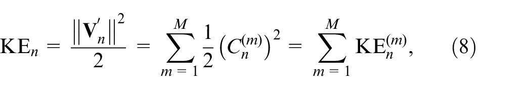
Consequently, the (specific) kinetic energy content of each fluctuation flow field (denote $\mathrm{K}{\mathrm{E}}_n$ for Cycle $n$ ) is also partitioned into each mode:

$$\mathrm{K}{\mathrm{E}}_n=\frac{{\Vert {\mathbf{V}}_n^{\prime }\Vert }^2}{2}=\sum _{m=1}^M\frac{1}{2}{\left(C_n^{(m)}\right)}^2=\sum _{m=1}^M{\mathrm{KE}}_n^{(m)},$$

(8)

where ${\mathrm{KE}}_n^{(m)}$ is the amount of kinetic energy of cycle $n$ collected by the $m$ th mode, which is equal to half of the squared Mode $M$ coefficient of Cycle $n$ ( $C_n^{(m)}$ ).

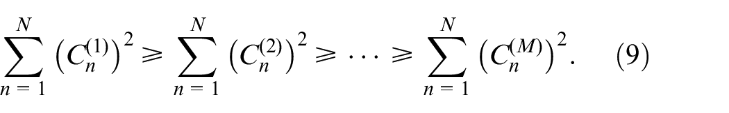
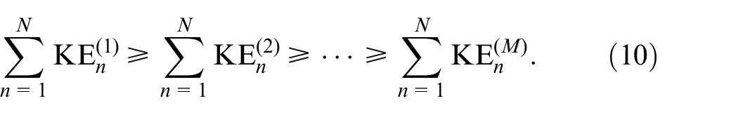
The POD modes are computed such that the sum of the squared coefficients are successively maximised from the first mode to the last (Mode $M$ ):

$$\sum _{n=1}^N{\left(C_n^{(1)}\right)}^2\ge \sum _{n=1}^N{\left(C_n^{(2)}\right)}^2\ge \cdots \ge \sum _{n=1}^N{\left(C_n^{(M)}\right)}^2.$$

(9)

Combining with equation (8), the kinetic energy content collected by each mode is also successively maximised:

$$\sum _{n=1}^N{\mathrm{KE}}_n^{(1)}\ge \sum _{n=1}^N{\mathrm{KE}}_n^{(2)}\ge \cdots \ge \sum _{n=1}^N{\mathrm{KE}}_n^{(M)}.$$

(10)

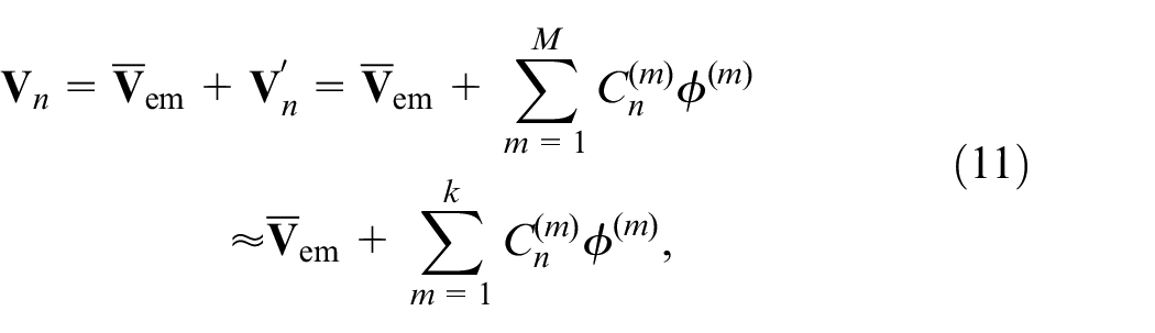
The underlying successive energy maximisation in POD bears immediate relevance to use the first $k$ ( $1\le k\le M$ ) terms in the decomposition (cf equation (6)) as a low-order approximation of the flow field for Cycle $n$ ⁵⁶ :

$$\begin{array}{c}{\mathbf{V}}_n={\overline{\mathbf{V}}}_{\mathrm{em}}+{\mathbf{V}}_n^{\prime }={\overline{\mathbf{V}}}_{\mathrm{em}}+\sum _{m=1}^M{C}_n^{(m)}{\varphi }^{(m)}\hfill \\ \approx {\overline{\mathbf{V}}}_{\mathrm{em}}+\sum _{m=1}^k{C}_n^{(m)}{\varphi }^{(m)},\hfill \end{array}$$

(11)

This approximation discards the low-energy (higher-order) terms (from the $(k+1)$ th to the $M$ th), and thus extracts the coherent structure (high energetic part) of the turbulent flow field. It should be noted that the ensemble mean must be included in the calculation so that the reconstructed fields can have comparable velocity magnitude with the original measured flow field. As such, the ensemble mean can be regarded as the zeroth-order approximation to all the cycles.

Although Chen et al.^55,57 recommends performing POD on instantaneous flow fields without subtracting the ensemble mean (i.e. POD on $\left\{{\mathbf{V}}_n\right\}$ ), it can also be argued that it is better to take the conventional Reynolds decomposition approach. Since the first POD mode of the instantaneous flow fields is an excellent estimate of the ensemble average (the $\mathrm{RI}$ value exceeds $0.99$ ), an unnecessary restriction will be added to the strongest fluctuation detected by the second POD mode of $\left\{{\mathbf{V}}_n\right\}$ – that this strongest fluctuation (and all the other modes) must be in a direction which is (almost) orthogonal to the ensemble mean since all the modes are strictly orthogonal to each other (equation (7)). On the other hand, by subtracting the ensemble mean prior to performing POD (i.e. POD on fluctuation flow fields $\left\{{\mathbf{V}}_n^{\prime }\right\}$ ), the first POD mode has no restriction in direction and can thus represent the main fluctuation flow structure to the greatest extent. Additionally, the differences when using either method are negligible in the context of this paper, since a number of POD components are added together to form the low-order approximated flow fields and hence the differences in the individual modes are diluted – the relevance index between the approximated flow fields (of the same cycle) using the two methods exceeds $0.92$ for all the $300$ cycles.

Comparison between RANS results and averaged PIV data

Ensemble mean

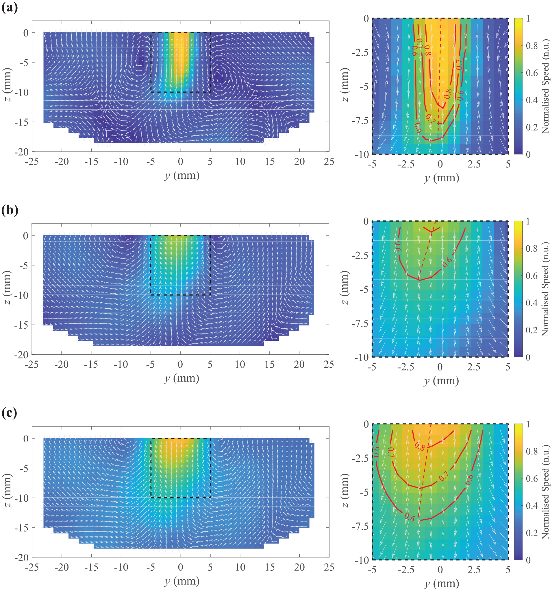
The ensemble mean flow field at $300$  CAD bTDCf (Figure 1(e)) is presented again in Figure 5(b) with a zoomed-in plot near the jet region. The flow speed inside the central jet region is notably slower than the RANS simulation (Figure 5(a), also plotted in Figures 1(f) and 4(a)). Again, if the simulation results were validated against the ensemble mean, one would easily conclude that the model over-estimated the jet speed. However, as visualised before in Figure 1(a) to (d), the actual jet speed in individual PIV cycles is much higher and closer to the RANS prediction.

Figure 5.

RANS simulated flow field versus averaged PIV flow fields at $300$ CAD bTDCf: (a) RANS simulation, (b) PIV ensemble mean and (c) PIV speed-based average.

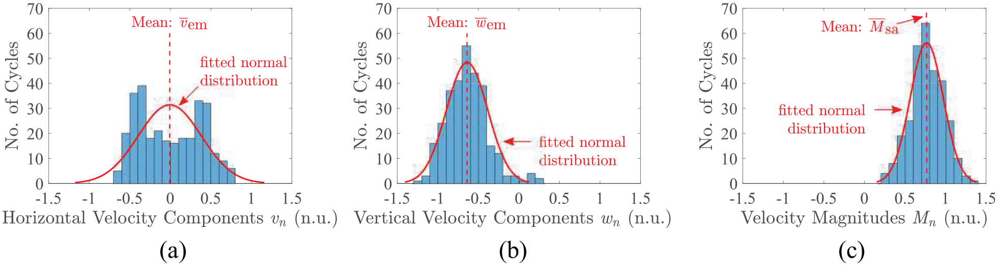
Careful examination of the velocity data measured on an example single point ( $y=0.19,z=-2.15$  mm) inside the jet region for $300$ cycles (Figure 6) suggest that large cyclic variation exists in the horizontal velocity components, for which the histogram (Figure 6(a)) has two peaks with comparable heights – both near $0.5$  n.u. (absolute values) but with opposite signs. Such a bimodal distribution is a classic signature of a flapping jet. The ensemble mean (equation (2)) averages out the horizontal velocity components, resulting in an almost zero horizontal speed ( ${\overline{v}}_{\mathrm{em}}=-0.0074$  n.u.). Its magnitude (equation (3)) is therefore much smaller than the jet speed of individual cycles.

Figure 6.

Speed distributions at a single point inside the jet region ( $y=0.19,z=-2.15$  mm) for $300$ cycles at $300$ CAD bTDCf: (a) histogram of $300$ horizontal velocity components, (b) histogram of $300$ vertical velocity components and (c) histogram of $300$ velocity magnitudes.

Viewed from another perspective, each of the two velocity components at a certain grid point can be regarded as a random variable, of which a histogram (Figure 6(a) for horizontal components, (b) for vertical ones) can be fitted by a normal distribution (red solid lines), and the validity of the fit can be examined by the chi-squared goodness-of-fit test. ⁵⁸ The horizontal components give a poor match ( ${\chi }^2(7,N=300)=102$ , $p\approx 0<0.05$ ), resulting from the swinging central jet that originated from the collision of the two intake streams; the vertical components generally follow the normal distribution ( ${\chi }^2(5,N=300)=7.6$ , $p=0.18>0.05$ ) and have negative values, showing that the majority of cycles have a downward central jet at that location. Consequently, using the vertical component of the ensemble mean to approximate the overall flow behaviour along the $z$ axis would be appropriate since it is equivalent to using the mean of a normal distribution to estimate the ensemble. Nevertheless, the same analogy cannot be applied for the horizontal component as the normal distribution assumption is no longer valid.

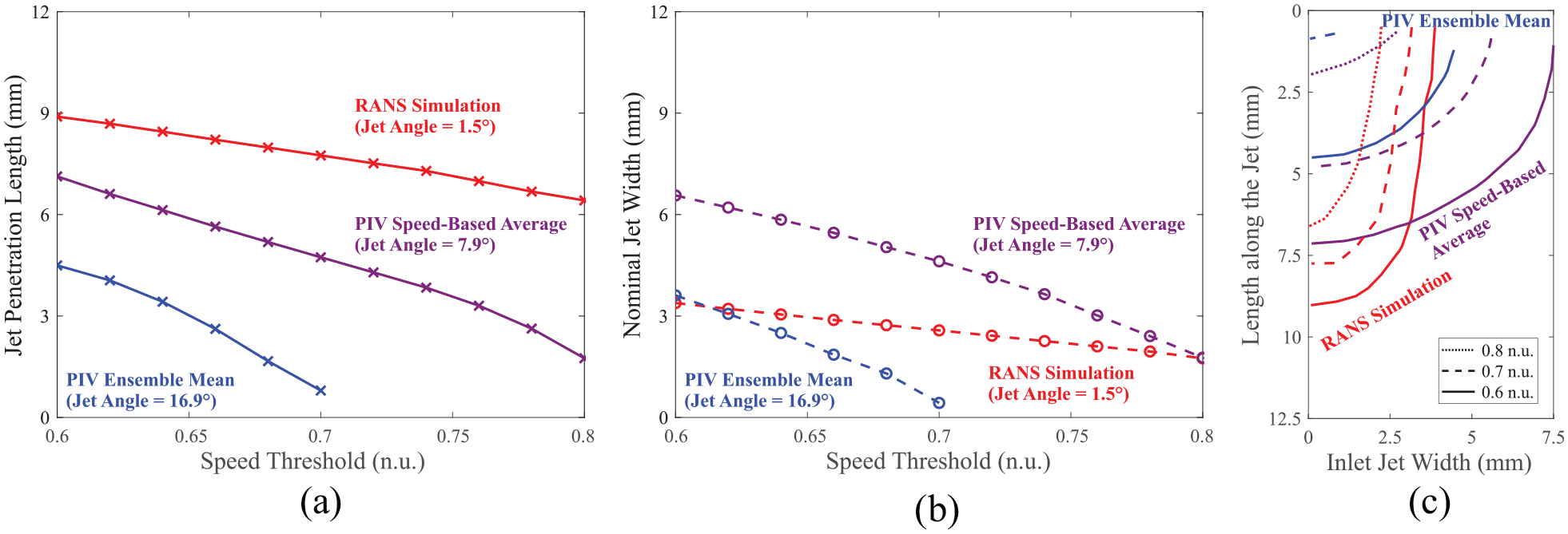
Quantifying the jet profile (Figure 7(a)) using the approaches defined in the earlier section also confirms that the ensemble mean has a much shorter jet penetration length (blue solid line with crosses) at any chosen speed threshold compared to the RANS model (red solid line with crosses). At higher speed thresholds (over $0.7$  n.u.), the jet profile (Figure 7(b)) for the ensemble mean is not even defined since it significantly under-represents the jet speeds present within individual cycles. As such, the ensemble mean would not be a suitable representation of the intake flow fields on the cross-tumble plane.

Figure 7.

Intake jet quantification metrics for the RANS simulated and averaged PIV flow fields at $300$  CAD bTDCf. (a) Jet penetration lengths, (b) nominal jet widths for RANS simulated (red), PIV ensemble mean (blue) and PIV speed-based averaged (purple) flow fields as functions of the speed threshold, (c) intake jet profiles (width as a function of length) at $0.8$  n.u. (dotted lines, at which the PIV ensemble mean is not defined), $0.7$  n.u. (dashed lines) and $0.6$  n.u. (solid lines) speed thresholds.

Speed-based averaging

The cancellation between horizontal components with opposing signs during calculation of the ensemble mean (Figure 6(a)) inspires an alternative approach – averaging the magnitude of vectors (speed) at each grid point. The speed of each vector is always non-negative, and therefore such so-called speed-based averaging avoids cancellation by negative values. The histogram of the velocity magnitudes (Figure 6(c)) at the previous example point inside the jet region matches with the normal distribution at $5$ % significance level ( ${\chi }^2(5,N=300)=10.47$ , $p=0.06$ ), and therefore its mean can be used as an approximation of the ensemble behaviour.

Figure 5(c) illustrates the speed-averaged flow field, of which flow direction is adopted from the ensemble mean (Figure 5(b)), while the colour map is replaced by the mean of magnitudes ( ${\overline{M}}_{\mathrm{sa}}$ , equation (4)). The flow speed inside the jet region is significantly higher than the ensemble mean, and is much closer to the actual jet speed measured in individual cycles Figure 1(a) to (d), as well as the RANS modelled data.

The jet profile in the PIV speed-averaged field, however, is quite different from the one in the RANS model. The speed-averaged jet (purple lines in Figure 7(a)) was found to have a smaller penetration length (solid lines with crosses) and a larger nominal width (dashed lines with hollow circles) than the RANS modelled jet (red lines). Both (purple) lines are steeper than the corresponding (red) lines for the RANS data, showing that the velocity gradients both along and perpendicular to the jet propagation direction are smaller, which is in line with the smoother jet profile observed in Figure 5(c) compared with the RANS simulation (Figure 5(a)). Additionally, as illustrated in Figure 7(b), its curvature (width as a function of length) is not similar to the RANS model. The RANS modelled jet (red lines) is ‘slim’ and has a ‘test tube-like’ curvature – the entry is not very wide, and the width almost remains constant until the tip of the jet, at which the width rapidly reduces to zero. The speed-averaged jet (purple lines), on the other hand, shows a ‘bowl-like’ curvature – it is much wider near the entry, and gradually shrinks as the length increases – as a result from the averaging of the swinging intake jet.

It should be noted that despite the speed-averaging method resolving the issue of under-representation of the intake jet speed, the background flow speed outside of the jet region is also increased compared to the ensemble mean. This is a direct result of the speed-averaging method since the directional fluctuations (whether cycle-to-cycle variations in the central jet structure or turbulent fluctuations across the flow field) no longer cause the flow speed cancellation, and any local high speed spots within individual flow fields, such as the one near ( $y=-10,z=-10$  mm) in Figure 1(c), will contribute towards the mean speed.

In addition to the flow speed and jet profile, some other flow features are also smoothed out by the two above-mentioned averaging methods, which makes the RANS validation questionable if they were used as validation targets. For instance, the intake jet applies a shear stress on the relatively slower in-cylinder flow, and creates so-called ‘shear vortices’ in the instantaneous flow fields (one of which is centred near $y=6,z=-6$  mm in Figure 1(a)). This flow feature is predicted by the RANS simulation (Figure 5(a)), but is smeared out in both averaging methods (Figure 5(b) and (c)) since the vortex centres in individual cycles may have different locations. The flow directions at the top-left and top-right corners of the PIV field of view also differ appreciably in direction ( $y$ components) between the RANS and the averaged PIV data using both methods. Given these disadvantages in using the averaged flow fields, they would not always be suitable choices as RANS model validation targets, especially when the highly-fluctuating intake jets are present.

Comparison between RANS Results and Low-Order POD reconstructed PIV Data

Low-order POD approximation of PIV data

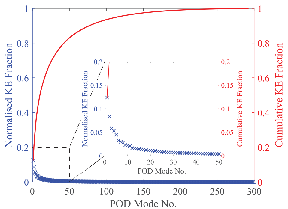
Proper orthogonal decomposition has been used widely to filter turbulent flow data and extract coherent structures from individual flow fields. This section aims to examine the possibility of validating a RANS simulated flow using approximated individual cycles by low-order POD reconstruction. Given the fluctuation flow fields at $300$ CAD bTDCf for $300$ engine cycles, POD (equation (6)) decomposes them into $299$ modes, ⁱ and also partitions their kinetic energy content in a successively maximised manner (equation (10)). As a result, the amount of kinetic energy distributed into each mode (blue crosses in Figure 8) decreases as the mode number increases. Most of the fluctuation kinetic energy is concentrated in lower order modes – the first ten modes (see cumulative sum in Figure 8) collected over $50$ % of the total kinetic energy, while less than $7$ % is in the last $200$ modes (Mode $100$ to the last). Therefore, it would be reasonable to approximate and extract the key features of the flow data in each cycle by reconstructing a field using the sum of several low order POD terms (equation (11)). One key question remaining to be answered would be, how many POD modes should be included in the reconstructed data to represent the coherent flow structure, without introducing small-scale turbulence that may bias its comparison with the RANS modelled data. The answer requires detailed observations to the approximated flow fields, which are discussed in the following paragraphs.

Figure 8.

POD kinetic energy spectra at $300$ CAD bTDCf with a zoom-in plot at lower-order modes.

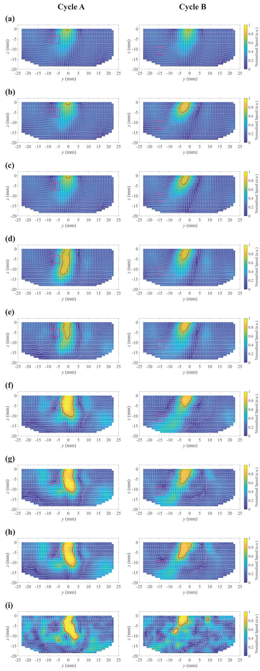
The POD reconstructed fields using different numbers of POD modes (equation (11)) for two arbitrarily selected engine cycles, Cycle A (Figure 1(a)) and Cycle B (Figure 1(b)), are shown in Figure 9. Each flow field has a $0.7$  n.u. contour highlighted in red marking the intake jet region and a magenta box ( $3\times 3$  mm) illustrating the vortex location of the original snapshot (Figure 9(i), bottom row) generated by the shearing flow from the central intake jet. It should be noted that the apparent flow patterns in individual POD modes (which for brevity are not shown here) do not represent actual flow features but only the relative strength of the fluctuations in different regions of the measured plane. The coherent flow structures in the instantaneous flow fields (Figure 9(i)) are instead preserved in the approximated flow fields (Figure 9(a)–(h)) once sufficiently large numbers of low-order POD components are added to the ensemble mean (cf equation (11)).^56,57 The focus of this paper lies only on the low-order approximated flow fields and thus discussions of the individual POD mode shapes are not presented.

Figure 9.

Approximated flow fields by low-order POD reconstruction for Cycle A (left column, cf Figure 1(a)) and Cycle B (right column, cf Figure 1(b)) at $300$ CAD bTDCf: (a) ensemble mean (0th-Order POD approximation), (b) 1st-order POD approximation, (c) 2nd-order POD approximation, (d) 3rd-order POD approximation, (e) 5th-order POD approximation, (f) 11th-order POD approximation, (g) 18th-order POD approximation, (h) 23rd-order POD approximation and (i) original snapshot (299th-Order POD ‘approximation’).

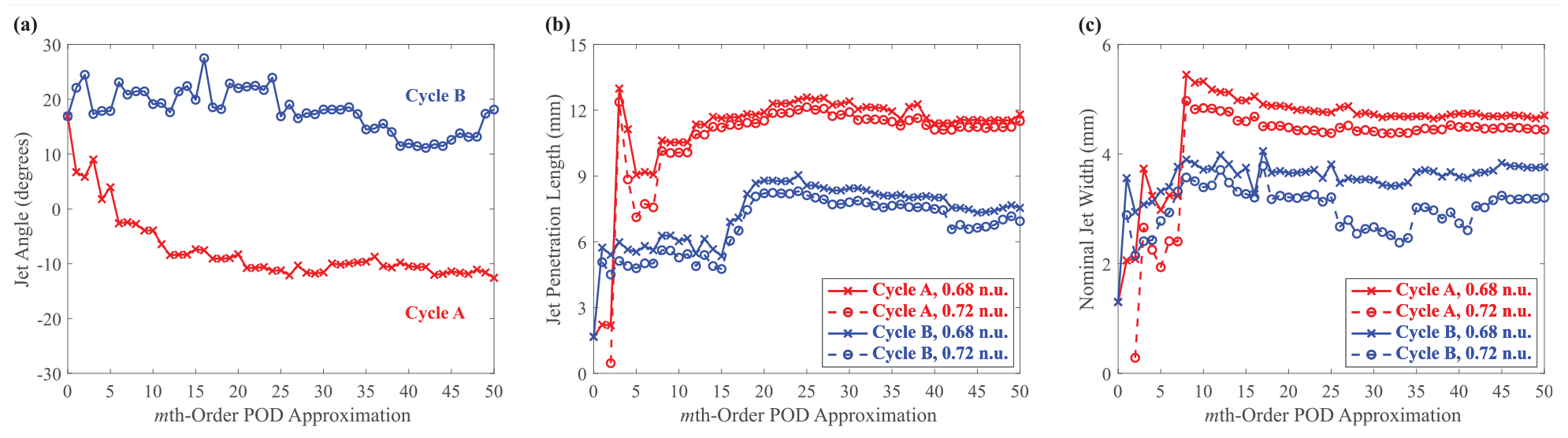
The jet profiles are quantified by the method previously discussed (Quantification of Intake Jet Profile), and the results can be referred to Figure 10, in which the jet angle (Figure 10(a)), jet penetration length (Figure 10(b)), and nominal jet width (Figure 10(c)) are each plotted as a function of the number of POD modes used in the approximation for Cycle A (red lines) and Cycle B (blue lines). Note that the jet angle (Figure 10(a)) is not a function of the speed threshold, while two speed thresholds around $0.7$  n.u. (solid line with crosses for lower speed threshold at $0.68$  n.u., dashed line with circles for higher speed threshold at $0.72$  n.u.) were chosen in order to show the robustness of the other two metrics (Figure 10(b) and (c)) versus the choice of speed threshold. The intake jet profile quantification used the $0.7$  n.u. speed threshold, and therefore the results would lie between the solid and the dashed lines in Figure 10(b) and (c).

Figure 10.

Intake jet quantification metrics for different orders of POD approximations at $300$  CAD bTDCf: (a) jet angle, (b) jet penetration length and (c) nominal jet width.

For both cycles, at a first glance, the approximated flow fields (Figure 9(a)–(h)) become closer to the original snapshot (Figure 9(i)) as more terms are included (from top to bottom), while differences still remain between the two cycles. For Cycle A (left column), adding the first two POD terms (Figure 9(b) and (c)) barely changes the intake jet profile from the ensemble mean (Figure 9(a), which is identical for both Cycles A and B, and was shown in Figures 1(e) and 5(b) before) – the intake jet speed is still under-estimated; the jet length is less than $2$  mm (Figure 10(b)) since the $0.7$  n.u. contour can only be seen at the top of the field of view. After adding the third term (Figure 9(d)), however, the jet profile changes significantly – despite the jet speed still being lower than the original snapshot (Figure 9(i)); their jet lengths are now comparable. The error in the shear vortex location (magenta boxes in Figure 9 ⁱⁱ ) is also within $2$  mm. However, the jet angle of the third term is positive (to the left, red solid line in Figure 10(a)), while the actual jet angle from the original snapshot ought to be negative (to the right, see Figure 9(i)). The reconstructed jet profile fluctuates strongly between the third- and the $11$ th-order of approximations (Figure 9(d)–(f)). For instance, at the fifth-order (Figure 9(e)), the contour illustrates a shorter and narrower jet region, and the values in the metrics also change rapidly from one approximation to the next (red lines in Figure 10). It should be noted that such apparently significant changes may, to a large extent, result from the slight magnitude changes around $0.7$  n.u. in the approximation, since the flow feature shown by the colour map and vectors is almost unaltered. On the other hand, the change does show that the flow speed inside the jet region is still fluctuating when more modes are included. After accounting for the $11$ th term (Figure 9(f)), the jet profile becomes more stable and evolves more gradually at higher-order approximations – only small changes can be observed visually from the $11$ th- to the $23$ rd-order approximations (Figure 9(f)–(h)), and the values of metrics (red lines in Figure 10) also converge to constants. For instance, the jet length is fluctuating between $10.6-12.5$  mm (slightly more than two vector spacings) from the $11$ th- to the $50$ th-order approximations. Therefore, Cycle A needs $11$ POD modes to represent its coherent flow structure.

Cycle B (right column), on the other hand, shows another trend in its low-order POD reconstructed flows. The sudden flow feature change by adding one mode (Mode $3$ for Cycle A) still exists but appears earlier – the first-order approximation (Figure 9(b)) illustrates a visible jet region with around $5.5$  mm jet length and $3.5$  mm nominal width at $0.7$  n.u. (blue lines in Figure 10(b) and (c)), as distinct from the zeroth-order (ensemble mean), which again almost has no jet region defined under this speed threshold. The ‘evolution’ of low-order approximations after the first-order (Figure 9(c)–(h)) appears to be very gradual, and the values of all three metrics (blue lines in Figure 10) change by small amounts. However, it is not until adding the $18$ th-order term (Figure 9(g)) to the approximation that the shear vortex starts to occur near the region of the original snapshot (highlighted by the magenta box). The jet penetration length also has a sudden increase (Figure 10(b)) before the $18$ th-order. Small differences in the jet profile can still be observed if more terms are added after the $18$ th-order (see, for instance, the $23$ rd-order approximation, Figure 9(h)), yet the change is considered to be negligible since most of the flow features (quantified in Figure 10) are already stable. As a result, $18$ modes are needed to provide a coherent structure of Cycle B.

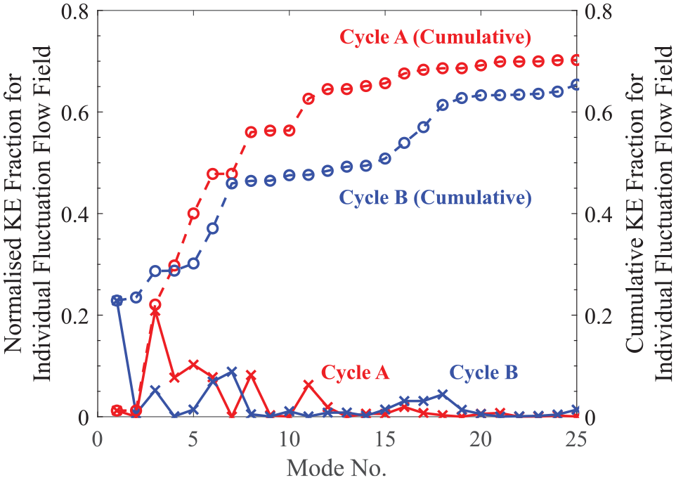
The reasons that different numbers of POD modes are needed for each cycle lie not only with cycle-to-cycle variation in the engine (i.e. in the measured PIV fields), but in the mechanism of the POD calculation as well. POD computes the modes by successively maximising the total amount of kinetic energy from all the $300$ fluctuation flow fields, so that the kinetic energy collected by lower order modes is always no less than the higher modes (equation (10)), yet the kinetic energy content of each cycle does not necessarily distribute into the modes in the successive maximisation manner. For instance, as shown in Figure 11, less than $2$ % of the kinetic energy of the fluctuation part of Cycle A is distributed into the first two modes (red lines), while Mode $3$ alone collects more than $20$ %, causing the sudden flow feature change mentioned previously from the second- to the third-order of approximations (left column of Figure 9(c) and (d); see also the metrics as red lines in Figure 10). A similar match between Figures 9 to 11 can also be found in the fluctuation velocity field of Cycle B (blue lines) – over $22$ % of its kinetic energy is in Mode $1$ , and the fraction does not exceed $9$ % in any of the remaining single modes. Therefore, one can expect the most noticeable change in flow structure would occur between the zeroth- (ensemble mean) and the first-order of approximations (right column of Figure 9(a) and (b), see also blue lines in Figure 10).

Figure 11.

Kinetic energy fraction collected by POD modes for Cycle A (red lines) and Cycle B (blue lines) at $300$  CAD bTDCf.

Additionally, as the kinetic energy of the fluctuation part of Cycle A rapidly accumulates ( $63$ % of total, red dashed line in Figure 11) in the first $11$ modes, the $11$ th-order POD approximation would have sufficient flow features to approximate Cycle A. The kinetic energy accumulation of the fluctuation part of Cycle B (blue dashed line), in contrast, is slower – although the first mode already has $22$ % of the kinetic energy and the percentage quickly increases to $46$ % in Mode $7$ , the cumulative kinetic energy fraction undergoes a very flat region with an additional seven modes only introducing another $3$ %, until it ramps up from $49$ % (Mode $14$ ) to $60$ % (Mode $18$ ). As a result, the change from different orders of approximation would be more gradual (right column of Figure 9), and Cycle B requires more modes in its reconstruction.

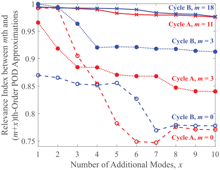
Other than the three intake jet profile quantification metrics, the ‘stability’ of each approximated field can also be evaluated by adding a number of extra components to a baseline approximation and calculating the directional similarity (quantified by the relevance index, cf equation (1)) before and after. The relevance indices between the $m$ th-order (baseline) and $(m+x)$ th-order approximations are computed and plotted in Figure 12 for Cycle A (red lines) and Cycle B (blue lines). When the baseline is set to be the ensemble mean ( $m=0$ ), adding one ( $x=1$ ) or two ( $x=2$ ) extra mode(s) does not change the flow structure for Cycle $\mathrm{A}$ (red dashed line with hollow circles, both $\mathrm{RI}>0.99$ ), while including the third component ( $x=3$ ) causes the $\mathrm{RI}$ to drop below $0.91$ , and the value continues to decrease as more components are added (increasing $x$ ). The values match with the previous findings by observing the approximated fields (left column of Figure 9) and the corresponding intake jet quantification metrics (Figure 10). Moving the baseline approximation to higher modes, say $m=3$ , one can further observe the effect of adding more modes to the third-order reconstructed flow of Cycle A (red dotted line with filled circles). The change of flow features is smaller (higher $\mathrm{RI}$ ), while the $\mathrm{RI}$ value still drops to $0.85$ after including eight more terms ( $x=8$ ), corresponding to the comparison with the $11$ th-order of approximation, showing that three modes are still not sufficient for the flow feature to stabilise. The calculation continues for higher order of baseline approximations, until at the $11$ th-order ( $m=11$ , red solid line with crosses), the $\mathrm{RI}$ values are higher than $0.97$ regardless of the number of extra components ( $x=1,2,\cdots ,10$ ), and thus the approximation of Cycle A stabilises at Mode $11$ .

Figure 12.

Relevance index between the $m$ th and $(m+x)$ th orders of POD approximations at $300$ CAD bTDCf for Cycle A (red lines) and Cycle B (blue lines). Each line uses a different $m$ value as the baseline when computing the $\mathrm{RI}$ values.

A similar procedure can also be implemented to Cycle B (blue dashed line with hollow circles) – the $\mathrm{RI}$ is below $0.87$ after introducing the first term to the ensemble mean ( $m=0$ , $x=1$ ) and reduces even further for higher orders ( $x>1$ ), which agrees with the appearance of the intake jet in the first-order POD approximation (right column of Figure 9) and the gradual change of the intake jet profile (blue lines in Figure 10) after the first mode. The flow feature is more but not sufficiently stable at $m=3$ – the minimum $\mathrm{RI}$ for all $x$ is higher than $0.91$ , yet a sudden drop of $\mathrm{RI}$ can be observed from $x=2$ (fifth-order approximation) to $x=4$ (seventh-order). At $m=18$ , all the $\mathrm{RI}$ values finally stay above $0.97$ , showing that the $18$ th-order POD reconstructed data for Cycle B is stable.

Zhuang and Hung ³⁴ took a similar approach when constructing the coherent structure in their quadruple POD analysis, except that they chose to set $x=1$ for their $100$ -cycle data set. For a large data set with $300$ snapshots ( $299$ computed POD modes) that include highly fluctuating intake jets, a larger $x$ value ought to be used in order to avoid the flow fields being apparently stable at lower order modes, since the flow features are more distributed in different modes and a single extra component may not be enough to change the flow structure. For instance, Cycle B would be falsely considered to be stable at its third-order approximation ( $m=3$ , blue dotted line in Figure 12) if only one extra mode ( $x=1$ ) is considered, since the $\mathrm{RI}$ is larger than $0.99$ . The actual decrease of $\mathrm{RI}$ that occurs after adding the Mode $7$ component ( $m=3$ , $x=4$ ), on the other hand, will not be observed.

Stability test of the low-order approximations

As exemplified by the previous paragraphs, determining the number of modes needed for a stable low-order reconstructed flow field of a specific cycle requires comprehensive evaluation on each order of approximation, which can be time-consuming to implement on a $300$ -cycle data set. Therefore, a stability test is proposed in order to automate this procedure. An $m$ th-order approximation is assumed to reach a stable flow structure if, comparing to the corresponding $(m+x)$ th-order approximations ( $x=1,2,\cdots ,10$ ), any four out of the five following criteria based on intake jet characteristics ( $1$ – $3$ ), kinetic energy content ( $4$ ) and overall vector-wise flow field direction ( $5$ ) are met:

1. the jet angle fluctuates within $\pm 5$ °;

2. the change of the jet penetration length is smaller than $1.68$  mm (twice the PIV vector spacing) at the $0.7$  n.u. speed threshold;

3. the change of the nominal jet width is smaller than $0.84$  mm (i.e. PIV vector spacing) at the $0.7$  n.u. speed threshold;

4. the difference in kinetic energy is smaller than $10$ % of the total kinetic energy collected by all POD components

5. the relevance indices are higher than $0.95$ with any of the choices of $x$ .

Among all the order of approximations for the same cycle which passed the above stability test, the one with the lowest order (i.e. uses least number of components) is chosen to be the approximated flow field of that cycle. The threshold of the nominal jet width is smaller than the one of the jet penetration length to compensate for their differences in absolute value ranges. The tests were conducted for a maximum of ten extra modes (denote $x$ ), assuming that the flow feature is unlikely to suffer a sudden change if it is already stable for ten extra components. It should be noted that the result from this stability test depends inevitably on choosing appropriate thresholds subject to the data set, yet this is considered to be reasonable since a similar subjective decision has to made when manually examining the flow fields.

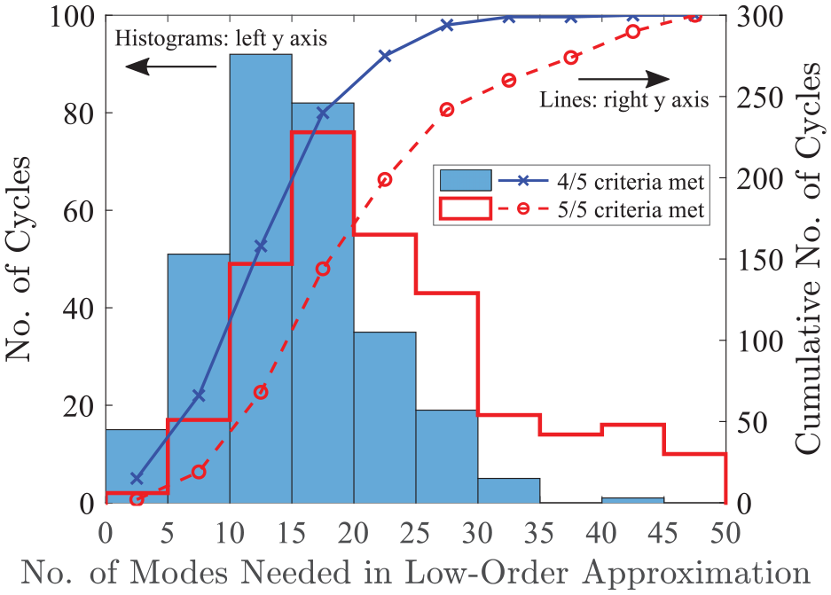
For all the $300$ cycles, the number of lower-order POD modes needed for each cycle is shown in Figure 13. Over half of the cycles require $10-20$  POD components (cf equation (6)) to reach a stable flow feature (blue filled histogram), and over $80$ % of them need fewer than $20$ components (blue solid line with crosses for the cumulative number of cycles), if four out of the five previously mentioned criteria are met. Take Cycle A (left column of Figure 9) as an example, the minimum number of modes needed to meet each criterion are: $11$ for jet angle (Figure 10(a)), $4$ for jet penetration length (Figure 10(b)), $8$ for nominal jet width (Figure 10(c)), $7$ for kinetic energy fraction (Figure 11) and $11$ for the relevance index (Figure 12). Therefore, the stability test suggests that the flow feature of Cycle A stabilises at the $11$ th-order approximation.

Figure 13.

Number of POD modes needed in low-order approximation for each cycle at $300$ CAD bTDCf identified by different numbers of criteria. Blue filled histogram and blue solid line: four out of the five stability test criteria are met; Red unfilled histogram and red dashed line: all the five stability test criteria are met.

The required modes increase when more constraints are put onto the stability test. For instance, if the test needs to meet all the five criteria instead of four, the majority of cycles would need about $15-25$ modes (red unfilled histogram in Figure 13), and the $80$ % cumulative line (red dashed line with hollow circles) shifts to $25-30$ modes. However, this may cause the stability test to over-constrain the results since the threshold for each criterion was used globally for all cycles but not all of them are always suitable for every cycle. Hence the previously proposed stability test only required meeting four out of the five criteria.

One way to examine whether the choices of thresholds are appropriate would be to see which criterion is most likely to be the ‘extra’ one – the one which was not accounted for in the stability test. Among all the $300$ cycles, $77$ of them have the jet angle as the unsatisfied criterion; the jet penetration length, nominal jet width and kinetic energy fraction each have $33$ , $37$ and $32$ cycles respectively; the relevance index criterion was not used in $82$ cycles; the remaining $39$ cycles have ‘tied’ criteria, meaning that multiple criteria give the same order of approximation and the extra one will not have any effect even if it was considered. (Cycle A is one of these $39$ cycles.) The results shows that the jet angle and relevance index thresholds may be too restrictive, resulting in the higher mode number when including the fifth criterion. Efforts may be made in the future to find a method that can choose the thresholds properly, such that most of the cycles have tied criteria and give a consistent number of modes, or make the five criteria equally restrictive (i.e. being the extra criterion for the same number of cycles). Additionally, the first three criteria (jet angle, penetration length and nominal width) were selected based on the specific flow features present on the measured plane during the intake stroke of this work. These criteria may not be applicable to other flow situations measured at a different crank angle or on another PIV plane. On the other hand, the other two criteria (kinetic energy difference and relevance index) are independent of the flow features, and thus can be applied to any flow field with appropriate selection of threshold values. It is recommended that the stability criteria should include both the flow features of interest and flow feature-independent metrics in other applications.

Validation of RANS simulated data using the low-order POD reconstructed PIV flow fields

The approximated flow field by low-order POD reconstruction extracts the key features and filters the small-scale turbulence and noise from the original PIV measurements, providing an alternative validation target for the RANS simulated data which were modelled based on averaged boundary conditions from the PIV experiments. Their similarity in terms of the intake jet profile can be again quantified by the metrics developed in an earlier section (Quantification of Intake Jet Profile), for which results are shown in Figure 14. Based on the stability test discussed in the previous section, Cycle A uses its $11$ th-order approximation, while Cycle B is reconstructed by $18$ POD components. For the readers’ convenience, the flow fields of the RANS simulation (Figures 1(f) and 5(a)), the PIV ensemble mean (Figures 1(e) and 5(b)), and the low-order POD reconstructed Cycle A (left column of Figure 9(f)) and Cycle B (right column of Figure 9(g)) are plotted again in Figure 15.

Figure 14.

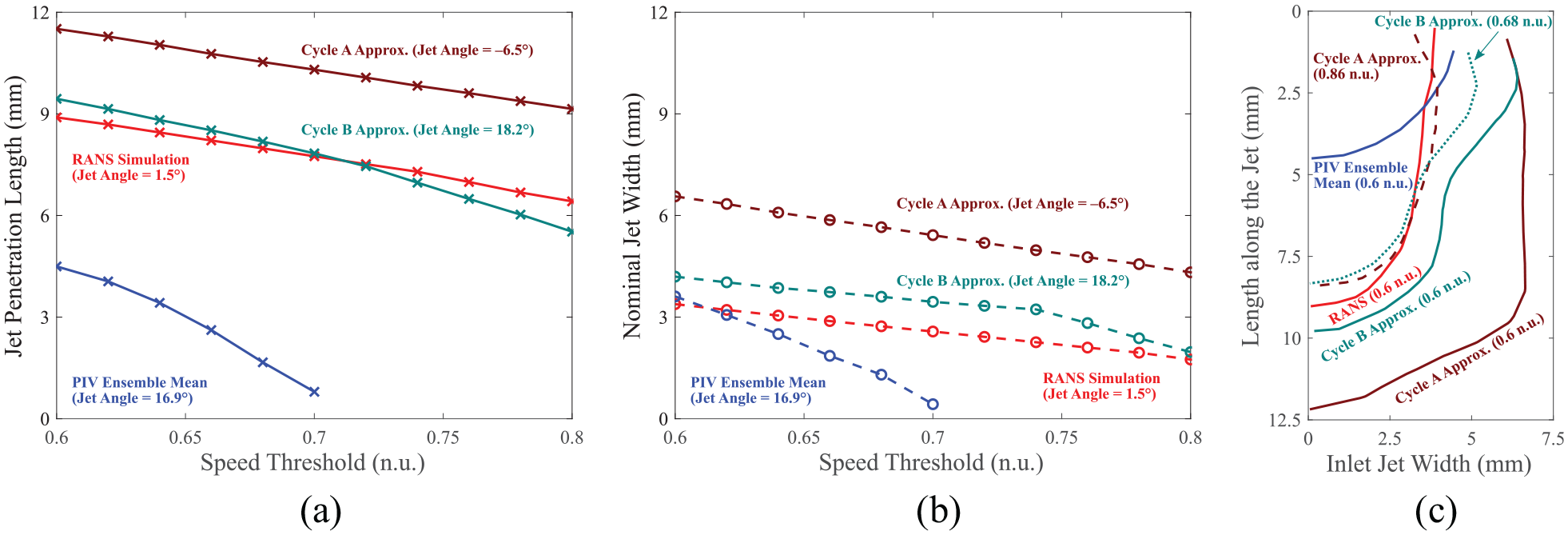
Intake jet quantification metrics for low-order POD approximated flow fields compared to RANS simulation and PIV ensemble mean at $300$ CAD bTDCf: (a) jet penetration lengths, (b) nominal jet widths for RANS simulated (red), PIV ensemble mean (blue), Cycle A’s low-order POD approximated (brown) and Cycle B’s low-order approximated (dark green) flow fields as functions of the speed threshold. The jet angles for each field are also reported and (c) intake jet profiles (width as a function of length) at $0.86$  n.u. (dotted line, Cycle A only), $0.68$  n.u. (dashed line, Cycle B only) and $0.6$  n.u. (solid lines) speed thresholds.

Figure 15.

RANS simulated flow field versus PIV ensemble mean and low-order POD approximated flow fields at $300$  CAD bTDCf. The red contour lines illustrate the jet region at $0.7$  n.u. threshold. These flow fields have been plotted in earlier figures: (a) RANS simulation, (b) PIV ensemble mean, (c) low-order POD approximation of cycle A, and (d) low-order POD approximation of cycle B.

The jet profiles of the low-order approximations of both cycles and the RANS model are comparable in many aspects. For Cycle A’s approximation, despite its jet penetration length (brown solid line with crosses in Figure 14(a)) at each speed threshold being larger than the corresponding value of the RANS model (red solid line with crosses), the slopes of the two lines are close, meaning that they have similar velocity gradients along the jet penetration direction. Similar observations can also be made for the comparison in the nominal jet widths as a function of the speed threshold (brown and red dashed lines with hollow circles in Figure 14(b)), showing the perpendicular velocity gradients of the approximated Cycle A and the RANS simulation are close to each other as well. As a result, the central intake jet of the Cycle A’s approximation (brown solid line in Figure 14(c); flow field shown in Figure 15(c)) has similar curvature with the one of the RANS simulation (red solid line in Figure 14(c); flow field shown in Figure 15(a)) – their width almost keeps constant in the main jet body, and the width rapidly shrinks to zero at the tip of the jet. However, one can also observe that the jet in the Cycle A’s approximation is much wider and longer at the same speed threshold ( $0.6$  n.u.).

Given the comparable velocity gradients and jet curvature, the relative characteristics of the RANS and low-order POD approximated PIV intake jets are well matched. By subsequently increasing the speed threshold of Cycle A’s approximation to find the best match versus the RANS simulated data, the scalar jet speed difference between the measurement and the simulation may be quantified. The best match was found at the $0.86$  n.u. speed threshold (brown dashed line in Figure 14(c)), at which the absolute values of the jet length and width of the Cycle A’s approximated flow field are in line with the RANS simulated data, in addition to the existing consistency in the intake jet curvature. Therefore, the speed difference inside the jet region is about $0.26$  n.u. Also, the jet angle calculation (mentioned previously in ‘Quantification of Intake Jet Profile’) shows that the jet angle difference between the approximated Cycle A and the RANS flow field is around $8^{°}$ (labelled in Figure 14(a) and (b)).

The low-order POD reconstructed flow field of Cycle B (Figure 15(d)) has almost the same jet penetration length (dark green solid line with crosses in Figure 14(a)) and slightly larger nominal jet width (dark green dashed line with hollow circles in Figure 14(b)) compared with the RANS simulated data (red lines in Figure 14(a) and (b)). The differences in the slopes of the corresponding lines are also small, showing that the velocity gradients are similar. Consequently, the central jet of the Cycle B’s approximation (dark green solid line in Figure 14(c)) has a profile that is close to the one of the RANS model (red solid line), and they have comparable length and width. It should be noted that, however, Cycle B’s approximation has a much wider jet at the entry compared to the RANS simulation. The jet speed difference between the approximated Cycle B and the RANS simulation is about $0.08$  n.u., which can again be estimated by increasing the speed threshold of Cycle B to $0.68$  n.u. (dark green dashed line in Figure 14(c)) and comparing to the RANS simulation (at $0.6$  n.u.). Despite these similarities, the jet angle (labelled in Figure 14(a)) of the reconstructed Cycle B deviates about $17°$ from that of the RANS simulation, which can also be observed by comparing their flow fields (Figure 15(d) vs (a)).

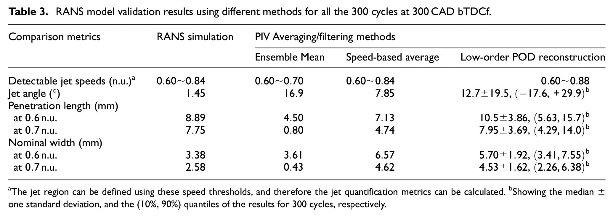
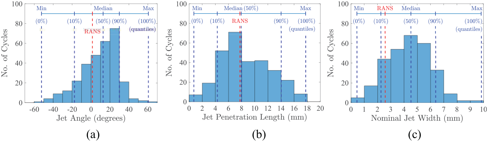
Viewing the entire $300$ -cycle dataset (Table 3 and Figure 16), the low-order POD reconstruction method provides a much fairer comparison to the RANS simulated data than using the other two averaging methods. The RANS model shows acceptable consistency with the coherent flow structures of the experimental data obtained by the low-order POD approximation, despite that it cannot provide information of the in-cylinder flow field cyclic variation. The jet regions for the RANS simulation and the low-order POD reconstructed flow fields can be defined at comparable jet speeds (detectable jet speeds in Table 3), albeit the jet speed is slightly lower in the RANS model. The jet length for the RANS model is close to the $300$ -cycle median of the low-order POD approximations (values reported in Table 3, see also a direct comparison in Figure 16(b)). While the RANS simulation predicts a smaller nominal width than the $300$ -cycle median, its value is still within the cyclic variation range (bounded by the $10$ % and $90$ % quantiles) of the experimental data (Figure 16(c)). The central intake jet profile of the RANS simulation and its velocity gradients are also in line with the corresponding properties for both example cycles (Figure 14). The mismatches with individual cycles, such as jet speed with Cycle A and jet angle with Cycle B, can easily be caused by the strong cycle-to-cycle variation in the flapping intake jet. For instance, the differences between the $10$ % and $90$ % quantiles of the jet angles for the low-order POD reconstructed flow fields are about ${38}^{°}$ in Table 3, and the jet angles for all the $300$ reconstructed flow fields span a range of ${112}^{°}$ in Figure 16(a), as a result of the uneven flow collision from the two intake valves.

Table 3.

RANS model validation results using different methods for all the $300$ cycles at $300$  CAD bTDCf.

Comparison metrics	RANS simulation	PIV Averaging/filtering methods
		Ensemble Mean	Speed-based average	Low-order POD reconstruction
Detectable jet speeds (n.u.) a	$0.60~0.84$	$0.60~0.70$	$0.60~0.84$	$0.60~0.88$
Jet angle (°)	$1.45$	$16.9$	$7.85$	$12.7\pm 19.5$ , $(-17.6,+29.9)$ b
Penetration length (mm)
at $0.6$  n.u.	$8.89$	$4.50$	$7.13$	$10.5\pm 3.86$ , $(5.63,15.7)$ b
at $0.7$  n.u.	$7.75$	$0.80$	$4.74$	$7.95\pm 3.69$ , $(4.29,14.0)$ b
Nominal width (mm)
at $0.6$  n.u.	$3.38$	$3.61$	$6.57$	$5.70\pm 1.92$ , $(3.41,7.55)$ b
at $0.7$  n.u.	$2.58$	$0.43$	$4.62$	$4.53\pm 1.62$ , $(2.26,6.38)$ b

a

The jet region can be defined using these speed thresholds, and therefore the jet quantification metrics can be calculated. ^bShowing the median ± one standard deviation, and the ( $10$ %, $90$ %) quantiles of the results for $300$ cycles, respectively.

Figure 16.

Intake jet quantification metrics for the $300$ low-order POD reconstructed cycles (blue) versus the RANS results (red) at $300$  CAD bTDCf. The jet penetration length and nominal jet width were evaluated at $0.7$  n.u. threshold; Statistical values were also reported in Table 3.

The RANS simulated flow field (Figure 15(a)) also captures several smaller-scale flow structures within the approximated PIV fields (Figure 15(c) for Cycle A and Figure 15(d) for Cycle B). For instance, the two shear vortices induced by the intake jet are centred respectively at $y=-6.56,z=-5.52$  mm and $y=+6.94,z=-7.21$  mm in the simulated flow field, which only deviates from the shear vortex centres in the Cycle A’s approximation ( $y=-7.40,z=-6.36$  mm and $y=+6.09,z=-6.36$  mm) by one vector spacing ( $0.84$  mm) in both $y$ and $z$ directions. The RANS-predicted flow directions in the lower-speed regions are also within the range of cyclic variations for the POD reconstructed fields. At the top-left corner of the PIV field of view, the RANS predicts a flow direction that is in line with the Cycle A’s approximation (inclined towards the positive $y$ direction), while slightly differs from the Cycle B’s approximation (inclined towards the negative $y$ direction). The flow directions for the RANS field and the approximations of both cycles are aligned near the top-right corner of the PIV field of view.

If the RANS model was validated only against the ensemble mean, it would be falsely considered as a poor model that significantly over-estimated the flow speed (much higher detectable jet speeds in Table 3). Other biased conclusions would also be drawn such that the model had a much longer intake jet (in Table 3 for two example speed thresholds, see other speed thresholds in Figure 14(a)), and even appeared to generate an incorrect jet profile (Figure 14(c)). Indeed, it was the ensemble mean (Figure 15(b)) itself that failed to be a representative flow field of the $300$ cycles – the jet length and nominal width for both speed thresholds are out of the corresponding ranges of the low-order POD reconstructions (Table 3), and the jet profile is significantly different from the original cycles (Figure 1(a)–(d)) or their approximations (Figure 15(c) and (d)). The speed-based averaging method generates closer values of the jet lengths and nominal widths to the RANS model and the low-order POD reconstructions (Table 3), but at the expense of an unavoidable background speed increase discussed in an earlier section (Speed-Based Averaging).

Additionally, the low-order POD reconstructions retain the variations of the jet quantification metrics in different measured cycles, and provide ranges of values that the simulation results should aim for. For instance, the $10$ % and $90$ % quantiles in Table 3 can be used as the validation lower and upper limits of the jet length and width. It should be noted that using the experimental median values as validation targets can sometimes be too restrictive – the RANS model only predicts a reference cycle without considering cyclic variations and hence the model can be considered accurate if the metrics fall within the corresponding experimental cyclic variation ranges (as illustrated in Figure 16(b) and (c)). On the other hand, the jet angles obtained from experiments vary significantly (Table 3 and Figure 16(a)) due to the flapping intake jet, making the resulting validation range overly large and easy for the RANS model to achieve. Therefore, caution is needed when interpreting the jet angle predicted by RANS models even if the value falls within the validation range (i.e. experimental cyclic variation range).

Summary and conclusion

The in-cylinder air charge motion on the cross-tumble plane was measured experimentally using particle image velocimetry (PIV) and also simulated by computational fluid dynamics (CFD) using the Reynolds averaged Navier-Stokes (RANS) turbulent model approach in a near-production spark ignition direct injection optically accessible engine. The purpose of this study was validating the modelled flow fields against the experimental measurements under highly-fluctuating flow conditions such as the engine intake process. Metrics were developed to quantify the profile of the central intake jet generated by the collision of the two intake air streams (from both valves), which allowed a detailed comparison between different flow fields containing the central intake jet. The RANS model simulates the flow fields by using the averaged boundary conditions from the PIV experiment, and it only generates one flow field at any fixed crank angle. Several methods were investigated to average the multi-cycle measured PIV flow fields to enable the validation. The conventional phase-averaged ensemble mean was first examined, yet its central intake jet was heavily affected by the horizontal velocity component cancellation due to the wide cycle-to-cycle variability of the flapping intake jet – the jet speed was found to be largely under-represented compared to individual PIV measurements and the jet profile was greatly smoothed such that it lacked key flow features and was not a representative flow field of the ensemble during the intake process. The speed-based averaging method resolved the issue of speed under-representation, but at the cost of introducing an unavoidable flow speed increase outside of the jet region, and the smoothing problem still remained. For instance, both averaging methods smear out the shear vortices induced by the intake jet which are present in the measured instantaneous flow fields.

These findings led to the necessity of using non-averaged individual PIV measured fields as RANS validation targets. These highly fluctuating flow fields must be filtered to allow a fair comparison with the non-fluctuating RANS simulation. Proper orthogonal decomposition (POD) was therefore implemented on the PIV data set, and the flow fields were reconstructed by using several low-order POD modes to extract the coherent flow structures and discard the smaller-scale turbulence and measurement noise. Efforts were made to find an appropriate cut-off mode number for the POD reconstruction based on key flow features in order to provide a robust approximation to the original measured flow fields, and a novel stability test was proposed to systemise the procedure. It is concluded that the low-order POD reconstruction is the most appropriate validation technique among the three methods presented in this paper. The reconstructed flow fields retained the major flow features of the central intake jet (such as the jet angle, penetration length, nominal width and jet-induced shear vortices) from the measured instantaneous flow fields, and also kept the cyclic variations in these metrics to provide reference ranges of values for a fair validation of the RANS simulated data. The results showed that the current RANS model provides a sufficiently accurate simulation in terms of the penetration length, the nominal width, the velocity gradients of the highly fluctuating central intake jet, as well as the location of the jet-induced shear vortices, though the jet speed is slightly under-estimated.

The methods developed in this paper can also be implemented on other data sets when the ensemble mean fails to be a good representation of highly fluctuating flow fields. Future focuses may involve finding best-matched PIV cycles versus the RANS simulation to examine whether the similarity in the intake jet profile during the early intake stroke ( $300$  CAD bTDCf) leads to similarity in later events such as mixture preparation after direct gasoline injection or flame propagation during the combustion, as well as modifying the RANS model based on the validation results.