Sage Journals: Discover world-class research

Abstract

Post-injection fuel dribble is known to lead to incomplete atomisation and combustion due to the release of slow-moving, and often surface-bound, liquid fuel after the end of injection. This can have a negative effect on engine emissions, performance and injector durability. To better quantify this phenomenon, we developed an image-processing approach to measure the volume of ligaments produced during the end of injection. We applied our processing approach to an Engine Combustion Network ‘Spray B’ 3-hole injector, using datasets from 220 injections generated by different research groups, to decouple the effect of gas temperature and pressure on the fuel dribble process. High-speed X-ray phase-contrast images obtained at room temperature conditions (297 K) at the Advanced Photon Source at Argonne National Laboratory, together with diffused back-illumination images captured at a wide range of temperature conditions (293–900 K) by CMT Motores Térmicos were analysed and compared quantitatively. We found a good agreement between image sets obtained by Argonne National Laboratory and CMT Motores Térmicos using different imaging techniques. The maximum dribble volume within the field of view of the imaging system and the mean rate of fuel dribble were considered as characteristic parameters of the fuel dribble process. Analysis showed that the absolute mean dribble rate increases with temperature when injection pressure is higher than 1000 bar and slightly decreases at high injection pressures (>500 bar) when temperature is close to 293 K. Larger maximum volumes of the fuel dribble were observed at lower gas temperatures (∼473 K) and low gas pressures (<30 bar), with a slight dependence on injection pressure.

Keywords

Diesel injector dribble ligament droplet shape atomization

Introduction

The end-of-injection (EOI) fuel dribble causes a formation of unburned hydrocarbons and decreases the performance of internal combustion engines in a variety of ways.¹ For example, deposits lead to an increase in air pollutant emissions,² a decrease in quality of injection^1,3,4 and further coking of the nozzle.⁵ Understanding the fuel dribbling process is particularly important for the development of a strategy for optimal use of fuels.⁶ However, observing the transient EOI processes is particularly challenging due to the extreme operating conditions and the microscopic scales involved. Consequently, there is a lack of quantitative information on the fuel dribble events and the parameters that affect them.¹

Recently published studies^7–10 demonstrate different aspects of the EOI fuel dribble based on a qualitative and quantitative analysis of experimental images of the injection process. The following important factors affecting the mechanism of the fuel dribble were studied: peak injection velocity, needle closing speed,⁸ in-cylinder pressure,^7,8 injection pressure,⁷ fuel mass expulsion and bubble ingestion at the EOI,¹⁰ liquid length recession at the EOI⁹ and different flow characteristics at the EOI.^11,12

Liquid phase penetration can be observed through several optical configurations that use visible-wavelength light as the source of illumination.^12,13 Light-scattering techniques capture the light elastically scattered by the liquid droplets through a high-speed camera.¹² At the same time, diffused back-illumination (DBI) systems allow observing the liquid phase, as this blocks the light incoming from the diffused source, but this optical configuration is limited to line of sight visualization. The recent introduction of fast light-emitting diodes (LED) improved the quality of the images gathered through DBI, because the duration of the light pulse can be set to very small values (nanoseconds). Thus, the amount of light available for each frame is governed by the pulse length of the LED, and not the exposure of the camera. Consequently, images gathered are significantly sharper than continuous light source options.^12–15

In addition to optical measurements using visible-wavelength light, high-speed X-ray imaging has been used extensively to study the morphology of fuel injection sprays.¹⁶ X-rays are highly penetrating in dense media, and scatter only weakly from liquid structures. This makes it possible to observe fluid structures inside the nozzle¹⁷ and features in the near field of the spray that are occluded due to multiple scattering of visible light. In X-ray phase-contrast imaging, weak diffraction at the interface of a droplet or ligament can be used to enhance image contrast when absorption in the liquid phase is poor. Using a high-flux, collimated synchrotron X-ray source, images of fuel injector spray structure can be made with several micrometres spatial resolution, and at a time resolution of tens to hundreds of microseconds with sub-microsecond effective image exposure times.¹⁶ X-ray phase-contrast images of fuel sprays are often difficult to interpret, as the complex structures present in the spray overlap in the projected image plane, and they are often blurred due to their high velocity. Under the conditions of post-injection fuel dribble, these problems are mostly avoided due to the low velocity and large size of the features.¹⁰ Under these relaxed conditions, the liquid structures have well-defined interfaces that infrequently overlap, and quantitative analysis of the liquid distribution becomes feasible. In this study, X-ray phase contrast is used to track the gas–liquid interface of droplets and ligaments formed due to injector dribble.

The present study is dedicated to a quantitative analysis of the fuel dribble with the focus on dribble volumes estimated by processing of images from high-speed X-ray phase-contrast and DBI imaging techniques within areas which correspond to fields of view of imaging systems (see Table 1). The three-dimensional (3D) reconstruction algorithm was developed to analyse volumes of the liquid when the fuel emerges from the orifice of the Engine Combustion Network (ECN) ‘Spray B’ injector. The main motivation of this investigation is to provide a better understanding of the parameters that influence the uncontrolled release of low-velocity fuel at the EOI.

Table 1.

Summary of experimental conditions for datasets used for analysis of the EOI fuel dribble.

Experimental conditions	CMT	Argonne
Injected liquid fuel	n-dodecane	n-dodecane
Injection pressure P_inj, [bar]	500, 1000, 1500	500, 1000, 1500
Ambient gas composition	nitrogen (pure)	nitrogen (pure); binary mixture nitrogen/helium (0.82/0.18 by mass)
Injector tip temperature	90°C	35 °C–40 °C at 500 bar; 60 °C–70 °C at 1500 bar
Gas temperature T_g, [K]	293, 473, 820, 900	297
Gas pressure P_g, [bar]	6.7–62	14.4, 30
Ambient gas density ρ_g, [kg/m³]	7.6–30	16.5, 34
ECN Spray B nozzle number	211200	211199
Number of the hole of interest	#3	#3
Nozzle hole diameter [µm]	93.2	90.9
Nozzle sac volume [mm³]	0.2	0.2
Frame exposure [µs]	8.33	1
Frame rate [Hz]	120000	67889
Scale factor [µm/pixel]	13.5, 4.8	5
Field of view [mm × mm]	6.91 × 2.16; 2.46 × 0.768	1.6 × 0.64

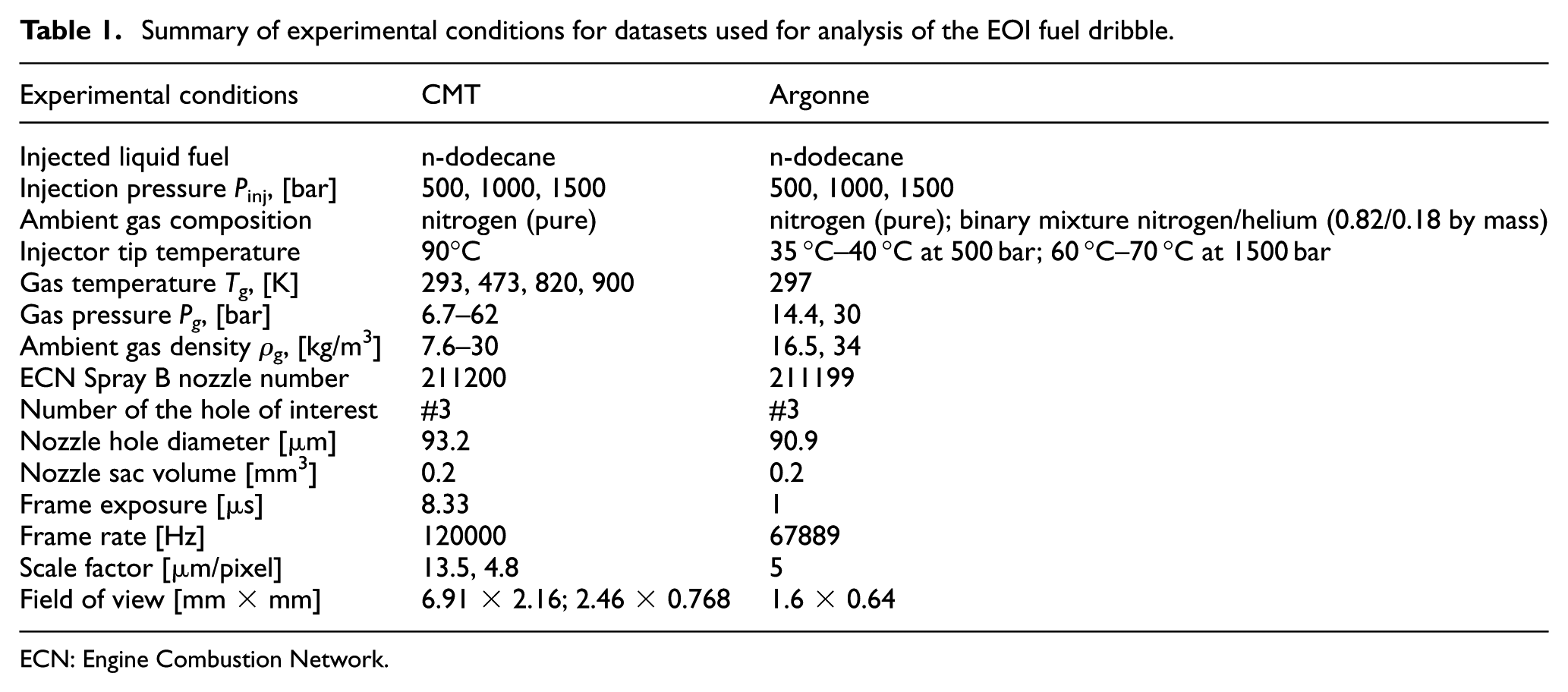
ECN: Engine Combustion Network.

Description of experimental methods

This study combines the analysis of videos from 220 injections of n-dodecane into a chamber where gas temperature and pressure were maintained within well-defined conditions. The main experimental parameters relevant to the study of the fuel dribble process are listed in Table 1.

Diffuse backlit illumination

DBI experiments were carried out at CMT Motores Térmicos of the Universitat Politècnica de València, using two high-pressures facilities: one at ambient temperature and one at high temperature. In the first facility,¹³ the test section was provided with a continuous flow of nitrogen from a high-pressure reservoir. A servo-operated valve, controlled by a closed-loop PID (proportional–integral–derivative), and located downstream of the spray chamber, manages the chamber pressure. Because the testing temperature is not controlled, the set point for the chamber pressure was continuously regulated to achieve constant density at given conditions. The second facility was also a constant pressure, low-velocity flow vessel but it was equipped with a gas heating system that provides the required temperature conditions. A description of the high-temperature facility can be found in recent works.^14,15

The optical configuration comprised a Photron SA-X2 camera equipped with a long-distance microscope lens. A diffusely illuminated background was achieved with a combination of a field lens and diffuser. The distance between the optical elements was set to maximize the diffusiveness of the background and to avoid beam steering, that is rarely observed in low-temperature conditions where little evaporation occurs, for example, the near nozzle region. The pulse length was set to 100 ns and pixel sizes of 13.5 µm or 4.8 µm, depending on the optical magnification and experimental campaign. The depth of field was estimated as 0.5 mm. A schematic diagram of the optical arrangement and an example of the experimental images gathered are presented in Figure 1.

Figure 1.

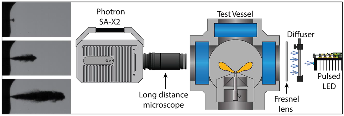
Schematic diagram of the diffused back-illumination experiments. The diagram is not to scale.

X-ray phase-contrast imaging

The X-ray phase-contrast experiments were performed at the 7-ID beamline of the Advanced Photon Source (APS) at Argonne National Laboratory.¹⁸ A schematic diagram of the facility is shown in Figure 2.

Figure 2.

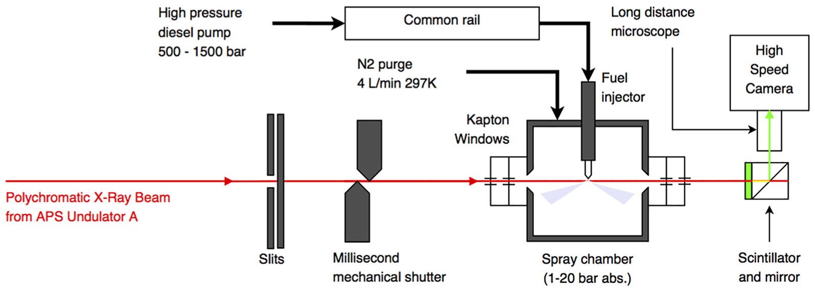
Schematic diagram of the X-ray phase-contrast imaging experiments. The diagram is not to scale.

The APS undulator A generated a polychromatic X-ray beam which was passed through a set of beam-forming slits, giving a field of view of approximately 1.6 mm (H) × 0.64 mm (V). The undulator gap^16–18 corresponds to the energy spectrum of the X-ray photons from the source, which defines the amount of absorption in the liquid. Observed in this study absorption is primarily due to photons at an energy of 11.8–13.1 keV (a single harmonic from the undulator source) with a bandwidth of approximately 2%–3% FWHM (full width at half maximum). The beam entered the 7-ID-B experimental station and passed through a pair of solenoid-actuated mechanical shutters. The beam then passed through a pressurized spray chamber fitted with Kapton (poly-oxydiphenylene-pyromellitimide) windows. A continuous 4 L/min (P = 30 bar) gas purge through the chamber cleared stray droplets between injections and prevented fluid build-up on the windows.

The diesel injector was mounted on a motorized translation stage in a horizontal position. Both the injector and the spray chamber were positioned accurately with respect to the X-ray beam, which was fixed in space. The beam passed by the tip of the nozzle, and some of the X-rays were absorbed and scattered by any fluid in the beam path. The scattered X-rays interfere with the incident beam in free-space propagation. A visible-light image was formed by a YAG scintillator placed approximately 30 cm downstream of the injector. A high-speed camera (Photron SA-4) fitted with a long working distance microscope recorded the images. The mechanical shutter was operated with a low duty cycle (30 ms exposure every 1 s) in order to reduce the heat load on the scintillator and nozzle due to absorption of the X-ray beam. The undulator gap was set between 25 to 31 mm. X-ray imaging was done at room temperature conditions. The pixel size was 5 µm². Further details are given in Table 1. In the operation mode of the APS undulator, each pulse of X-rays had a period of 27 to 50 picoseconds, which was sufficiently fast to freeze the flow. The electronic global shutter on the camera was opened for 1 µs, catching a train of multiple exposures separated by a period of 500 ns. Thus, the motion blur was not severe for observed ligaments and droplets.

Methodology of the image analysis

3D reconstruction

The extraction of size and shape from two-dimensional (2D) images of droplets, particles, liquid ligaments or tree-like structures is used in a number of industrial applications such as medical imaging and so on.^19–21 Similarly to previously published algorithms,²² the present analysis is based on the estimation of object cross-sections from a line-based structure of an initial image followed by the smoothing of the 3D shape. The present study is based on the object model demonstrated in Figure 3a. A circular assumption for object cross-sections allowed reconstruction of the 3D shape using the limited information available from individual 2D images. As a result, the image processing algorithm does not involve any fixed axis of symmetry for all reconstructed ligaments and droplets. Numbers of pixels in each row of the binarized image were treated as diameters of circular cross-sections of the object of interest.

Figure 3.

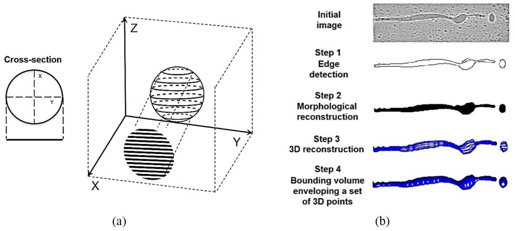
(a) Schematic of the object model and (b) main steps of the image processing algorithm. X-ray phase-contrast image was used to show different steps of image processing (see initial image).

The image processing algorithm consisted of the following stages (Figure 3b):

Edge detection consisted of complex image binarization algorithms which are able to identify edges in the presence of flickering background and noise.

2D morphological reconstruction for filling gaps in previously detected edges. Intermediate stage: Line-based structure of binary image is used to calculate characteristics of object cross-sections.

3D reconstruction. Coordinates of 3D points are calculated based on centres and radii of cross-sections.

Computation of the bounding volume which envelops a set of 3D points – alpha shape.

The image processing approach was applied to both experimental techniques: high-speed X-ray phase contrast and DBI. Three different edge detection methods were used to remove background and noise from experimental images: Canny algorithm,²³ wavelet filter and morphological opening.

The choice of the Canny edge detector was motivated by its excellent performance in the presence of flickering background and boundaries which are caused by a combination of X-ray absorption and phase-contrast effects.²⁴ Since the detected edges usually have gaps, a Delaunay triangulation algorithm²⁵ was applied for 2D reconstruction of contours from multiple objects. Compared to the X-ray imaging, the DBI method provided similar light intensity values for each pixel which belongs to the liquid phase.¹³ DBI videos were processed using a transformation which consisted of a convolution of the images with a wavelet filter, followed by a thresholding. The wavelet filter detects concavity and convexity of the grey level variation in the image.²⁶ Edges from the DBI images were also processed by morphological opening with erosion followed by dilation, using the same structuring element for both operations. Details related to the application of morphological operations to greyscale images were discussed elsewhere in the literature.^26,27 Following recommendations from literature,^26–29 the adjustable parameters for each edge detection method were chosen depending on a number factors: size and number of objects, type of background noise, movements of the image background and image contrast.

The intermediate stage of the image processing algorithm uses the row-based structure of binary images. The detection of the liquid used pixel slices along the rows of the images (in the direction normal to the spray axis) to determine equivalent diameters and centre coordinates of each slice.

The centre and diameter of each slice, together with a parametric equation for a circle, were used to build a 3D point cloud for each cross-section (slice) of the object, in a plane orthogonal to the image plane. Merging all available ‘slices’ generates a 3D array which represents the shape of the full object. At the last stage of 3D reconstruction, a smooth surface is obtained by computation of the bounding volume enveloping the 3D point cloud – the alpha shape. The definition of the alpha shape in 3D space can be found elsewhere in literature.^30,31 There are three main parameters necessary to build the alpha shape: alpha radius, region threshold and holes threshold. Depending on a value of the alpha radius, the alpha shape can transform from concave into a convex object. Larger values of alpha radius usually result in convex objects. Recommendations regarding the choice of the alpha radius for correct representation of the 3D shape were discussed elsewhere.³¹ The region threshold allows the maximum number of objects in the 3D array to be determined. Finally, the hole threshold reduces the number of defects and holes in the alpha shape.

Verification of the 3D reconstruction algorithm

For this initial approach at modelling the 3D morphology of microscopic droplets and ligaments, we have made two simplifying assumptions: the liquid structures are axisymmetric and aligned with the pixel array. While these assumptions preclude the 3D modelling of completely arbitrary shapes, they can be justified by the experimental configurations used in the present study.

The above circular assumption for object cross-sections can be justified by the fact that the experiments were performed with the spray axis aligned with the image plane, and both surface tension and momentum limit the formation of asymmetric liquid structures in the plane orthogonal to the spray axis. This is particularly the case when liquid velocities are small, which is to be expected for X-ray phase contrast and DBI experiments performed during the EOI. Although this assumption cannot be easily verified since measurements for the depth of the fuel structures were not available, this study is based on the hypothesis of slow-moving ligaments and droplets.

The 3D reconstruction algorithm was verified by calculation of the surface area (S) and volume (V) from synthetic 2D images of simple shapes: sphere, cylinder and spheroid. The average relative error was chosen as a measure of accuracy in the calculations of S and V. The description of test shapes and errors are summarized in Table 2. A cylinder, sphere, prolate and oblate spheroids were considered as models for liquid ligaments and droplets. Two half-spheres were attached to the cylinder to model a typical shape of a ligament.

Table 2.

Average relative error in calculations of volume and surface area for different test shapes.

Description of test shapes	Volume error (%)	Surface area error (%)
Sphere	4.7	3.4
Prolate spheroid. A = 0°	2.7	1.9
Prolate spheroid. A = 1°	6.5	4.3
Prolate spheroid. A = 5°	7.6	4.9
Prolate spheroid. A = 12°	11	7.6
Prolate spheroid. A = 21°	13	10
Prolate spheroid. A = 29°	30	24
Oblate spheroid. A = 90°	8.3	45
Prolate spheroidand sphere	16	6.4
Cylinder with two hemispherical caps	0.6	0.1
Two spheres separated by 0.05D	14	0.8
Two spheres separated by 0.15D	14	1.6
Two spheres separatedby 0.2D	19	5.9

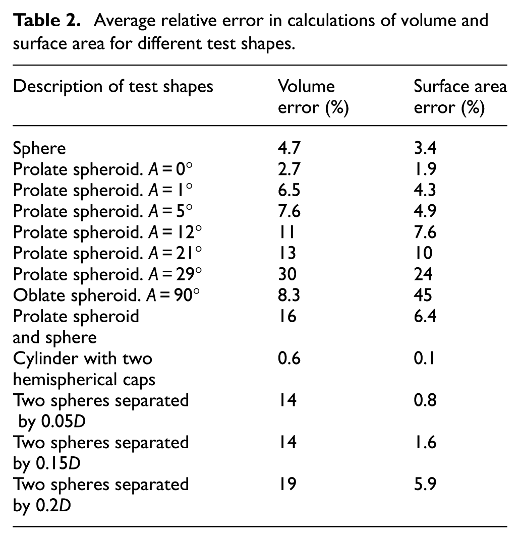
Average relative errors in calculations of V and S for spherical objects were found to be 4.7% and 3.4%, respectively. Inclined spheroids were chosen to simulate the rotation of ligaments in images of the fuel dribble. As is seen in Table 2, the largest relative error in calculations of V and S is observed in cases when the inclination angle of the major axis of the spheroid (A) equals 29 degrees. It should be mentioned that the most accurate reconstruction of the 3D shape was observed for the objects which were vertically oriented along the spray major axis, a cylinder with two hemispherical caps, confirming that the approach is reasonably accurate for the liquid structures being studied. Two spheres with different distances between their centres were chosen as models of the droplet pinch-off phenomenon. Current analysis showed that the change of the distance between two spheres produces errors which equal 19% and 5.9% for V and S, respectively. In addition, a combination of prolate spheroid and sphere was also considered as the model for the initial stage of the pinch-off effect.

The assumption that liquid structures are aligned with the pixel array was made to simplify the slice-by-slice reconstruction process. This assumption was satisfied by ensuring that the spray axis was aligned with the pixel array, either during the image acquisition or by rotation of the acquired images. The effect of rotation of spheroid structures with respect to the pixel array is quantified in Table 2, and as expected larger errors are obtained for angles that significantly deviate from the images’ axes. It should be mentioned that such large errors are expected to be rare in this study, as the majority of ligaments were well aligned with the image (i.e. spray) axis.

Results and discussion

Time dependence of the fuel dribble volume

Examples of results of the 3D reconstruction and raw images are shown in Figure 4. The reconstructed liquid structures are presented in blue on the left of Figures 4(a) and (b). The nozzle orifice is located near the top of both figures.

Figure 4.

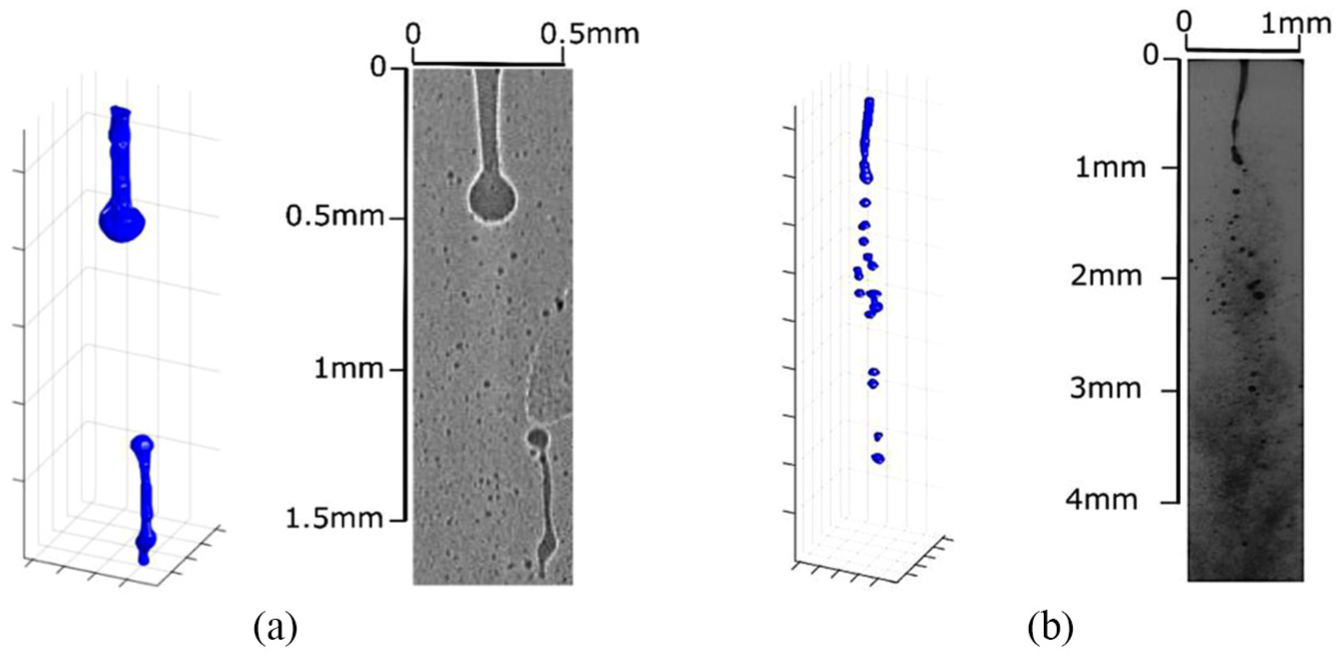
Raw images with results of 3D reconstruction, from (a) X-ray phase-contrast technique (P_inj = 500 bar; P_g = 30 bar; T_g = 297 K) and (b) DBI image (P_inj = 500 bar; P_g = 27 bar; T_g = 293 K). Images (a) and (b) were captured after 132.6 µs and 333 µs after the end of injection.

The present analysis required the separation of the dribble events from the main injection stage, when a finely atomized spray is formed. As can be seen in Figure 5, the liquid volume present in the region of interest increases rapidly at the beginning of the injection stage and reduces almost to zero when the needle of the diesel injector is closed (after 2 ms in Figure 5). The volume of liquid present in the region of interest then increases again due to the dribble process. The image analysis shows that the relative duration of dribble events varied from 5% to 23% of the time between opening and closing of the injector needle.

Figure 5.

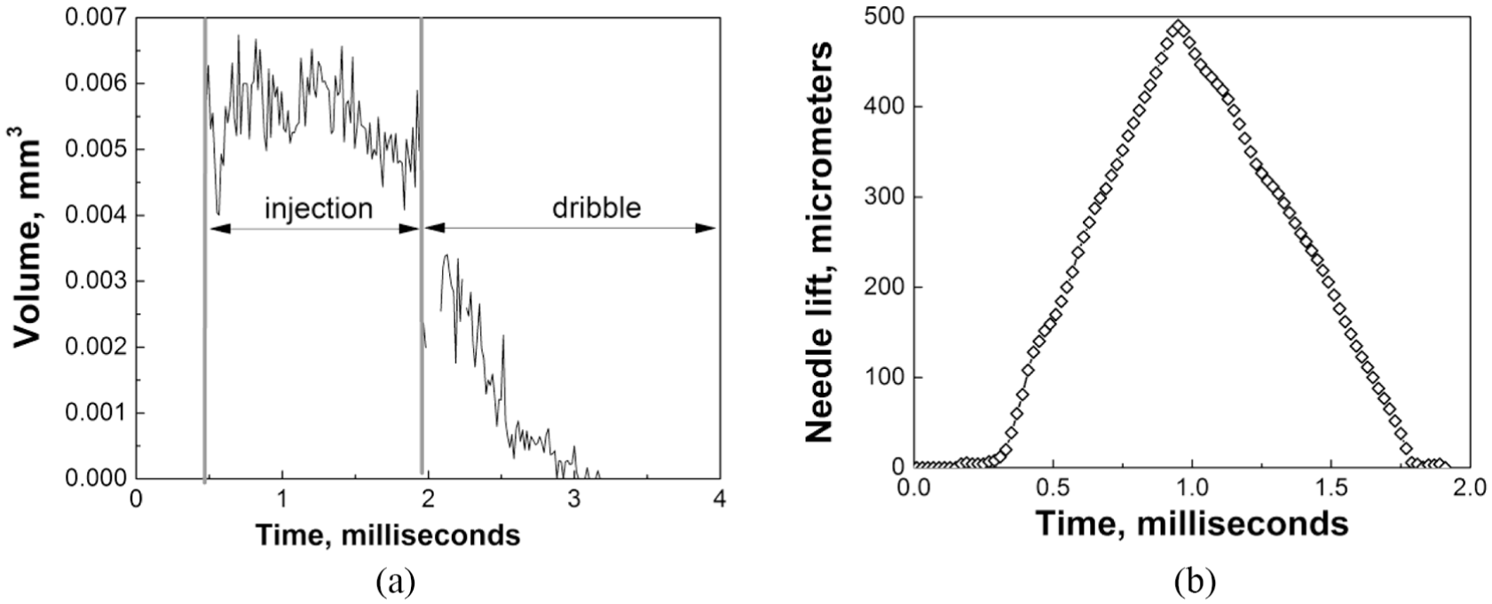
Time dependence of the liquid volume during the injection process for: P_inj = 1500 bar, T_g = 297 K and P_g = 20 bar. (a) Experimental data and (b) needle lift values are provided by Argonne.

As can be seen in Figure 6, both the volume (V) and external surface area (S) of the liquid structures present in the field of view increase rapidly to a maximum value during the first stage of the dribble process. The initial increases in V and S relate to the fuel being released from the orifice after the end of the main injection event. Both volume and surface area then gradually decrease during the second stage (Figure 6a). Dashed lines in Figure 6 represent high order polynomial fitting of time evolution for V and S. Time dependences of dribble volumes were fitted with polynomials which allowed to find the maximum dribble volumes for each analysed injection. The decrease in these quantities is related to both the reduction in the volume flow rate of dribble, and the disappearance of some of the liquid structures from the region of interest, as they move out of the field of view of the imaging systems. All dribble events showed similar behaviour with respect to changes in liquid volume and surface area. Since all dribble image sequences demonstrated this behaviour, the maximum dribble volume was considered as a characteristic parameter of the process.

Figure 6.

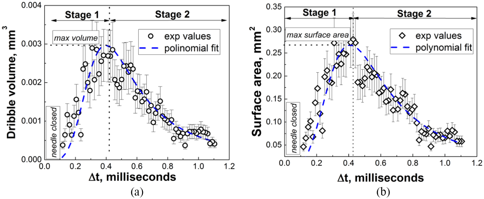
Dribble volume (left image) and surface area (right image) versus time. Both diagrams obtained by processing of X-ray images which correspond to the following conditions: P_inj = 1000 bar, T_g = 297 K and P_g = 30 bar.

In agreement with previously published studies,^7,8 our investigation revealed a high cycle-to-cycle variation in the quantity of fuel delivered after the EOI (Figure 7). In order to reduce the effect of cycle-to-cycle deviation in results obtained at the same experimental conditions, dribble volumes from different injections were pre-processed by removing outlier points with deviations larger than three standard deviations from the mean value. These outliers were an artefact of the image processing algorithm, rather than a characteristic behaviour of the dribble event. Time values in Figure 7 were calculated using as a reference the moment of time when the injector needle was closed. The mean dribble volumes were calculated by averaging experimental volumes calculated at the same instants in time. The curve based on median values is shown in Figure 7 by the blue line. Further analysis of time dependences of the dribble volume was done using curves with median volumes calculated at the same experimental conditions. As shown in Figure 8, there is an acceptable agreement between median dribble volumes calculated at similar experimental conditions using images from Argonne and CMT. The same as in Figures 6 and 7, time differences in Figure 8 were calculated using as the reference the moment of time which corresponds to needle closure. As can be seen in Table 1, field of view sizes for sets of images by CMT and Argonne are different. The field of view for CMT images was reduced in order to make comparison of dribble volumes in Figure 8 at similar conditions.

Figure 7.

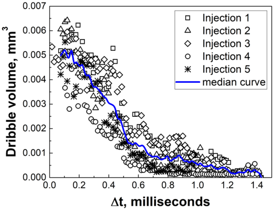
Time dependence of dribble volumes obtained from Argonne data for the following experimental conditions: P_inj = 500 bar, T_g = 297 K, P_g = 30 bar and ρ_g = 34 kg/m³. Obtained dribble volumes correspond to a sequence of injections which were obtained at similar experimental conditions.

Figure 8.

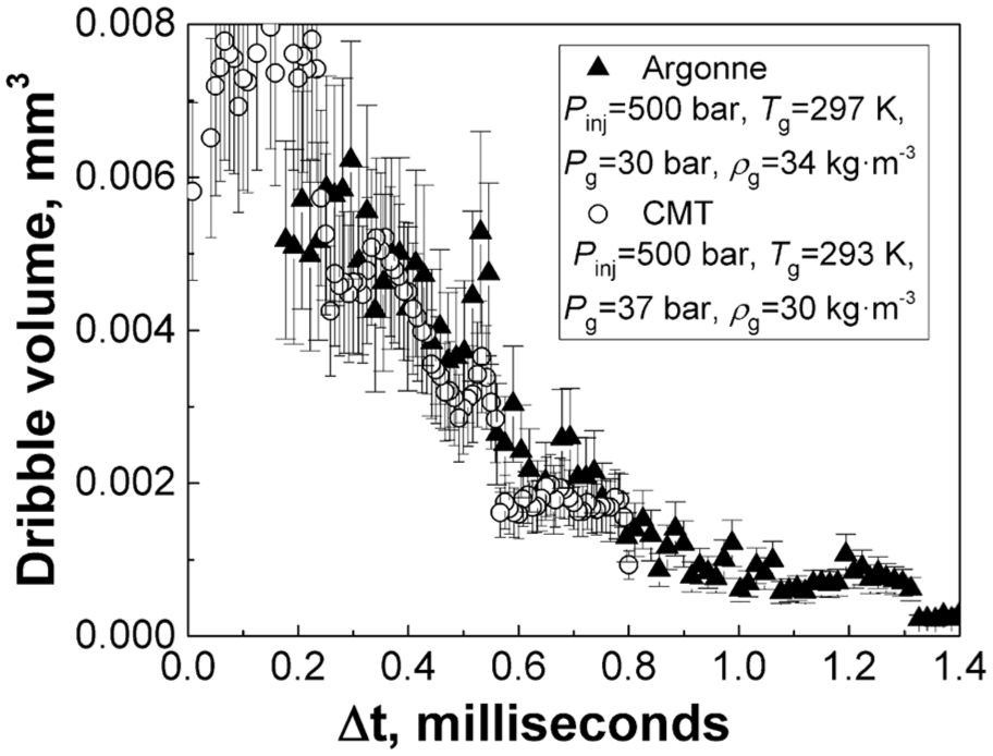
Comparison of median dribble volumes obtained at similar experimental conditions using sets of images from Argonne and CMT.

Further quantitative analysis of the fuel dribble process is based on the approach which uses time dependences of median dribble volumes at different experimental conditions. Applied methodology of analysis of fuel dribble process consists of the following steps:

Time dependences of dribble volumes were averaged using images from sequences of injections which were acquired at similar values of injection pressure, gas temperature and gas pressure. As a result, median curves of dribble volumes are obtained (see example in Figure 7).

Median curves of dribble volumes were fitted using high-order polynomial equations.

Fitting curves were used to identify maximum dribble volumes.

Median dribble volumes at the second stage of the dribble process (see Figure 6) were used to calculate dribble rate values.

Maximum dribble volumes

The above analysis of the image processing results allowed to conclude that the maximum values in time dependences of the dribble volumes (Figure 6) reveal some dependence on the experimental conditions which occur during injections. Considering the above, this study uses the maximum dribble volume as a characteristic metric of the dribble process at different values of injection pressure, gas temperature and gas pressure. Maximum dribble volumes were considered as an additional metric which plays a role in the analysis of the rate of the fuel dribble. Similar to the integral dribble volume, the maximum dribble volume in Figure 6 allows to identify which conditions promote larger post-injection fuel losses – injection pressure, gas temperature or gas pressure. The main drawback of the maximum dribble volume as a characteristic of post-injection fuel losses is a difficulty in such practical applications as a development of the strategy for optimal use of fuels, for example. Instead of total volume of fuel losses after the injector needle closure, the maximum dribble volume provides a local maximum point on the curve which represents a time dependence of the fuel dribble process. In this study we assume that the maximum dribble volume is proportional to the integral dribble volume which cannot be calculated with acceptable level of accuracy using images by CMT and Argonne.

The maximum dribble volumes obtained from various experiments by CMT and Argonne at room temperature (293–297 K) are in good quantitative agreement (Figure 8), suggesting that the fuel volumes estimated from the morphological reconstruction are consistent. No clear dependence of the fuel dribble on injection pressure was observed (Figure 9), although the lowest injection pressure tested (500 bar) seemed to generate relatively more dribble at room temperature conditions. However, the volume measurements for high gas temperatures are less consistent (Figure 9), and thus it is more difficult to identify a clear overall dependence of the fuel dribble on injection pressure. One may argue that fuel injection pressure should be expected to have no direct effect on the release of fuel after the nozzle has been closed. At the same time, higher injection pressures are known to lead to higher gas volume fractions in the nozzle (through cavitation), which in turn should reduce the volume of liquid trapped inside the nozzle and orifices after needle closure.

Figure 9.

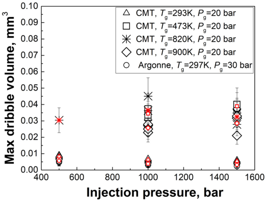
Dependence of maximum dribble volume on injection pressure P_inj. Averaged values of the maximum dribble volume are shown by red symbols.

The above-mentioned analysis shows that gas temperature has a significant impact on the volume of fuel dribble (Figure 10). Measurements performed by CMT at elevated temperatures (473–900 K) were found to generate 2 to 4 times more dribble after the end of the main injection event, for all injection pressures (Figure 10). Interestingly, the largest volume of fuel dribble was recorded for mid-range temperatures (473 K). This may suggest that at room temperature the high viscosity of the liquid prevents some of the fuel from dribbling out of the nozzle. As the gas temperature is increased (and the viscosity and surface tension of the liquid reduced), a larger volume of fuel can flow out of the injector orifice. Since the dribble process is affected by momentum, it is also expected that the lower gas densities at high gas temperatures (for a fixed gas pressure) could lead to the larger amount of fuel being released from the nozzle. As the gas temperature is further increased to 820–900 K, the trend reverses and the measured dribble volume somewhat reduces (Figures 9 and 10a), indicating that other parameters are affecting the process. We note that the apparent reduction in measured dribble volume at high temperatures could be related to increased evaporation at these conditions, rather than a net reduction in released liquid volume.

Figure 10.

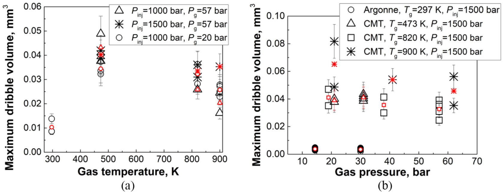
Dependence of the maximum dribble volume on (a) gas temperature T_g and (b) gas pressure P_g. Averaged values of the maximum dribble volume are shown by red symbols.

This investigation shows that the increase of gas pressure reduces the dribble volume (Figure 10b). Such behaviour is expected to be related to the increase in gas density, providing more resistance to the flow of fuel out of the injector’s orifices. It also suggests that the larger volume of fuel dribble occurred at low engine gas temperatures (∼473 K) and low gas pressures, with little dependence on injection pressure. It is interesting to note that these findings are in good agreement with recent results showing an increase in the emission of unburnt hydrocarbons for these engine conditions.³²

Volumetric flow rate of fuel dribble

Median curves (Figure 7) obtained after pre-processing of time dependences of the dribble volume were used to calculate volumetric flow rates in the fuel dribble process. A rate of disappearance of the liquid structures from the field of view of the imaging systems was used as a measure of the rate of the fuel dribble:

R_{i} = \frac{(V_{i + 1} - V_{i})}{(t_{i + 1} - t_{i})}

(1)

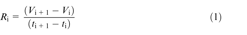
where R_i is the dribble rate, which was computed from two consecutive video frames from the same injection in m³ s^–1; V is the dribble volume in m³; t is time in seconds; i is the index of the frame in the time-sequence.

Both sets of images by CMT and Argonne demonstrate large number of small droplets (≤5 µm) remaining during the first stage of the fuel dribble process just after the injector needle was closed. The above analysis showed that similar intensities of pixels which correspond to droplets formed in the moments before and just after the needle closure affect significantly the accuracy of dribble volume calculations (see Figure 11). Due to large errors in volume calculations (more than 40%) in the presence of residual droplets, the analysis of the dribble rate behaviour was only performed for the second stage of the dribble process (Figure 6). The image analysis showed that the instantaneous dribble rate R_i does not change significantly during the second stage of the fuel dribble process.

Figure 11.

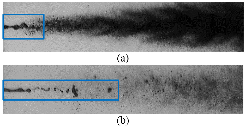
Raw DBI images obtained at (a) 160 µs and (b) 2.4 ms after the closure of the injector needle. Dribbling fuel is highlighted by the blue rectangles. Top and bottom images correspond to following experimental conditions: P_inj = 500 bar, P_g = 26 bar and T_g = 293 K.

Time dependent values of the dribble rate R_i were averaged to calculate the parameter which characterizes the dynamics of the fuel dribble process – the absolute mean dribble rate:

R_{m} = | \sum_{i = 1}^{N} \frac{R_{i}}{N} |

(2)

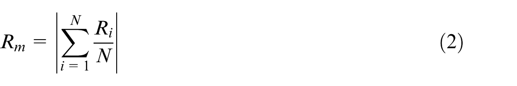
where $R_{m}$ is the absolute mean dribble rate in m³ s^–1; N is the number of data points, which depends on the duration of the dribble process and the exposure time of the camera.

Similar to the liquid flow rate during the fuel dribble process, the absolute mean dribble rate in equation (2) allows to identify which conditions promote faster fuel losses after the injector needle closure – injection pressure, gas temperature or gas pressure. The main drawback of the R_m is a difficulty in practical application. R_m provides a volume per time unit after the maximum dribble volume has been reached (Figure 6). This study is based on the above-mentioned assumption that the dribble rate (equation (1)) during the second stage of the dribble process does not change with time almost until the end of the dribble process. It should be mentioned that, despite the fact that the above principle of the separation of the fuel dribble process in two stages was verified using experimental images by CMT and Argonne, it is required to study if our approach is valid for multi-hole injectors at realistic conditions which correspond to dynamic changes of temperature and pressure.

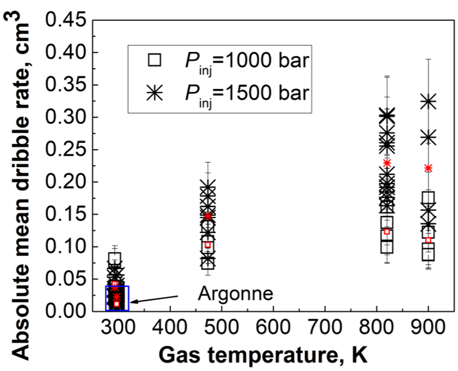
$R_{m}$ ranges from zero to –0.3 cm³ s^–1. In order to verify this approach, we can observe that the dribble events last 1.5 ms (Figures 5 –8) and knowing the nozzle sac volume (0.2 mm³) we can establish that the theoretical volume flow rate for the full discharge of the nozzle sac is 0.13 cm³ s^–1. This theoretical flow rate is close to the values in Figure 12, suggesting that our estimation of the absolute mean dribble rate from the video frames is reasonable.

Figure 12.

Dependence of the absolute mean dribble rate on the gas temperature T_g. Argonne data are highlighted by the blue rectangle. Averaged values of the absolute mean dribble rate are shown by red symbols.

This analysis shows that the gas temperature T_g has a significant impact on the $R_{m}$ (Figure 12). Measurements performed at elevated temperatures (473–900 K) demonstrated significantly larger $R_{m}$ after the end of the main injection event. Comparison of the absolute mean dribble rates computed from injections at the same values of P_inj and T_g shows a high sensitivity of $R_{m}$ to changes in the gas and nozzle tip temperatures (Figure 12). At elevated injection pressures (1000–1500 bar), the discrepancy between absolute mean dribble rates at room temperature conditions is 2–4 times smaller compared with the high-temperature experiments (473–900 K). At the same time, it should be mentioned that injections at P_inj = 1500 bar revealed the smallest dribble rate throughout the range of temperatures from 293 to 900 K. The analysis of injections at low values of P_inj (<500 bar) suggests that there is a significant decrease of the absolute dribble rate at room temperature conditions (Figure 13). Direct comparison of Figures 12 and 13 allows to conclude that, at low temperatures (293 K), the reduction of the injection pressure leads to significantly higher absolute mean dribble rates. Examination of time dependences of dribble volumes computed at similar gas pressures P_g = 20 ± 1 bar and at elevated gas temperatures (473–900 K) allows to detect a small increase of $R_{m}$ at injection pressures higher than 1000 bar (Figure 13).

Figure 13.

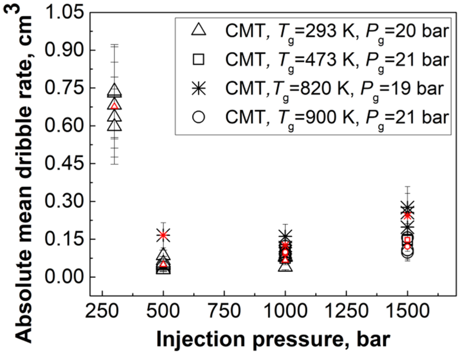
Dependence of the absolute mean dribble rate on injection pressure. Averaged values of the absolute mean dribble rate are shown by red symbols.

Summary and conclusion

A quantitative investigation of fuel injector dribble using 3D morphological reconstruction of liquid structures using high-speed videos recorded at Argonne (X-ray phase-contrast) and CMT Motores Térmicos (DBI) was performed. Our quantitative analysis allowed to get similar results using images acquired by two different research institutions. In addition to the previously published study of the fuel dribble through the mechanism of spreading of the surface-bound fuel around the orifice,³³ this study is focused on the fuel overspill through the separation of droplets and ligaments from the nozzle orifice within areas which correspond to fields of view of imaging systems (see Table 1). This study allowed us to estimate the volume of liquid released from one orifice of a three-hole ECN ‘Spray B’ injector and the absolute mean dribble rate during the injection.

The largest dribble volume flow rates were observed at low injection pressures (less than 500 bar) and room temperature conditions (∼293 K). At the same time, our analysis showed the absolute mean dribble rate also slightly increases with temperature when injection pressure is higher than 1000 bar.

We found that the larger volumes of fuel dribble occurred at lower engine gas temperatures (∼473 K) and low gas pressures (<30 bar), with little dependence on injection pressure. These findings are in good agreement with recent results showing an increase in the emission of unburnt hydrocarbons for these conditions³² and a quantitative study of the spreading of the surface-bound fuel around the nozzle orifice.³³

The results of the post-injection fuel dribble were obtained from injections which were observed from one orifice of the injector. It is necessary to confirm the temperature and pressure dependencies when experimental data for the fuel dribble from all three holes of the injector become available.

Footnotes

Appendix 1 Acknowledgements

The authors would like to thank Team Leaders Gurpreet Singh and Michael Weismiller for their support of this work. The authors wish to thank the anonymous reviewers for their insightful comments and constructive criticisms which helped improve and clarify this article.

Declaration of conflicting interests

The author(s) declared no potential conflicts of interest with respect to the research, authorship, and/or publication of this article.

Funding

The author(s) disclosed receipt of the following financial support for the research, authorship, and/or publication of this article: The image processing research was supported by the United Kingdom’s Engineering and Physical Science Research Council (Grants EP/K020528/1 and EP/M009424/1) and BP Formulated Products Technology. The X-ray measurements were performed at the Advanced Photon Source at Argonne National Laboratory. Use of the Advanced Photon Source (APS) is supported by the U.S. Department of Energy (DOE) under Contract No. DEAC02-06CH11357. The X-ray component of this research was partially funded by DOE’s Vehicle Technologies Program, Office of Energy Efficiency and Renewable Energy.

ORCID iDs

Vitaliy Sechenyh

Raul Payri

Cyril Crua

References

Sandquist

Denbratt

Owrang

Olsson

. Influence of fuel parameters on deposit formation and emissions in a direct injection stratified charge SI engine. SAE technical paper 2001-01-2028, 2001.

Caprotti

Fowler

Lepperhoff

Houben

. Diesel additive technology effects on injector hole erosion/corrosion, injector fouling and particulate traps. SAE technical paper 932739, 1993.

Birgel

Ladommatos

Aleiferis

Zülch

Milovanovic

Lafon

, et al. Deposit formation in the holes of diesel injector nozzles: a critical review. SAE technical paper 2008-01-2383, 2008.

Orley

Hickel

Schmidt

Adams

. Large-Eddy Simulation of turbulent, cavitating fuel flow inside a 9-hole diesel injector including needle movement. Int J Engine Res 2017; 18(3): 195–211.

Argueyrolles

Dehoux

Gastaldi

Grosjean

Levy

Michel

, et al. Influence of injector nozzle design and cavitation on coking phenomenon. SAE technical paper 2007-01-1896, 2007.

Benajes

Novella

De Lima

. Analysis of combustion concepts in a newly designed two-stroke high-speed direct injection compression ignition engine. Int J Engine Res 2015; 16: 52–67.

Turner

Stetsyuk

Crua

Pearson

Gold

. The effect of operating conditions on post injection fuel discharge in an optical engine. In: Proceedings of the 13th triennial international conference on liquid atomization and spray systems, Tainan, Taiwan, 23–27 August 2015.

Moon

Huang

Wang

. End-of-injection fuel dribble of multi-hole diesel injector: comprehensive investigation of phenomenon and discussion on control strategy. Appl Energ 2016; 179: 7–16.

Kook

Pickett

Musculus

. Influence of diesel injection parameters on end-of-injection liquid length recession. SAE Int J Engine 2009; 2: 1194–1210.

10.

Swantek

Kastengren

Duke

Tilocco

Sovis

Powell

. A further examination of fuel dribble from single hole diesel nozzles. In: Proceedings of the ILASS Europe, 26th Annual Conference on Liquid Atomization and Spray Systems, Bremen, 8–10 September 2014.

11.

Kastengren

Powell

Tilocco

Liu

Moon

Zhang

, et al. End-of-injection behaviour of diesel sprays measured with X-ray radiography. J Eng Gas Turbines Power 2012; 134: 094501.

12.

Manin

Bardi

Pickett

Payri

. Boundary condition and fuel composition effects on injection processes of high-pressure sprays at the microscopic level. Int J Multiphase Flow 2016; 83: 267–278.

13.

Payri

Bracho

Gomes-Aldaravi

Viera

. Near field visualization of diesel spray for different nozzle inclination angles in non-vaporizing conditions. Atomizat Spray 2017; 27(3): 251–267.

14.

Gimeno

Marti-Aldaravi

Carreres

Peraza

. Effect of the nozzle holder on injected fuel temperature for experimental test rigs and its influence on diesel sprays. Int J Engine Res 2018; 19(3): 374–389.

15.

Payri

Salvador

Manin

Viera

. Diesel ignition delay and lift-off length through different methodologies using a multi-hole injector. Appl Energ 2016; 162: 541–550.

16.

Duke

Matusik

Kastengren

Swantek

Sovis

Payri

, et al. X-ray radiography of cavitation in a beryllium alloy nozzle. Int J Engine Res 2017; 18(1–2): 39–50.

17.

Duke

Swantek

Sovis

Powell

Kastengren

Fezzaa

. Recent developments in X-ray diagnostics for cavitation. SAE Int J Fuel Lubricant 2015; 8(1): 135–146.

18.

Walko

Adams

Doumy

Dufresne

March

, et al. Developments in time-resolved X-ray research at APS beamline 7ID. AIP Conf Proc 2016; 1741: 030048.

19.

Fessler

Macovski

. Object-based 3-D reconstruction of arterial trees from magnetic resonance angiograms. IEEE Trans Med Imag 1991; 10: 25–39.

20.

Cárdenes

Novikov

Gunn

Rod

Frangi

. 3D reconstruction of coronary arteries from rotational X-ray angiography. In: International Symposium on Biomedical Imaging, Barcelona, 2–5 May 2012. New York: IEEE.

21.

Goyal

Prakash

Yang

. 3D reconstruction of coronary arteries from angiographic images: a survey. Int J Comput Sci Netw 2013; 2(3): 96–101.

22.

Hoffmann

Doi

Chan

Chua

. Computer reproduction of the vasculature using an automated tracking method. Proc SPIE Med Imag 1987; 767: 449–453.

23.

Canny

. A computational approach to edge detection. IEEE Trans Pattern Anal Mach Intell 1986; PAMI-8(6): 679–698.

24.

Kastengren

Tilocco

Duke

Powell

Zhang

Moon

. Time-resolved X-ray radiography of sprays from engine combustion network spray a diesel injectors. Atomizat Spray 2014; 24(3): 251–272.

25.

Delaunay

. Sur la spheäre vide. A la meä moire de Georges Voronoiä. Bulletin de l’Académie des Sciences de l’URSS. Classe des sciences mathématiques et naturelles 1934; 6: 793–800.

26.

Fdida

. Développement d’un système de granulométrie par imagerie: application aux sprays larges et hétérogènes. Thèse de doctorat en Physique, Université de Rouen, Mont-Saint-Aignan, 2008.

27.

Serra

. Image analysis and mathematical morphology. Orlando, FL: Academic Press, 1983.

28.

Igbinosa

. Comparison of edge detection technique in image processing techniques. Int J Inform Tech Electric Eng 2013; 2(1): 25–29.

29.

Shrivakshan

Chandrasekar

. Comparison of various edge detection techniques used in image processing. Int J Comput Sci 2012; 9(5): 269–276.

30.

Edelsbrunner

Mucke

. Three dimensional alpha shapes. ACM Trans Graph 1994; 13(1): 43–72.

31.

Lafarge

Pateiro-López

Possolo

Dunkers

. R implementation of a polyhedral approximation to a 3D set of points using the α-shape. J Stat Soft 2014; 56(4): 1–18.

32.

Koci

Dempsey

Nudd

Knier

. Understanding hydrocarbon emissions in heavy duty diesel engines combining experimental and computational methods. SAE Int J Engine 2017; 10(3): 1093–1109.

33.

Turner

Sykes

De Sercey

Stetsyuk

Gold

Pearson

, et al. A quantitative analysis of nozzle surface bound fuel for diesel injectors. In: Proceedings of the ILASS Europe, 28th European Conference on Liquid Atomization and Spray, Valencia, 6–8 September 2017.

Quantitative analysis of dribble volumes and rates using three-dimensional reconstruction of X-ray and diffused back-illumination images of diesel sprays

Abstract

Keywords

Introduction

Description of experimental methods

Diffuse backlit illumination

X-ray phase-contrast imaging

Methodology of the image analysis

3D reconstruction

Verification of the 3D reconstruction algorithm

Results and discussion

Time dependence of the fuel dribble volume

Maximum dribble volumes

Volumetric flow rate of fuel dribble

Summary and conclusion

Footnotes

Appendix 1

Acknowledgements

Declaration of conflicting interests

Funding

ORCID iDs

References