Sage Journals: Discover world-class research

Abstract

Biodegradable metals have gained attention in the field of bone repair, to be used as temporary bone implants. Among those metals, iron shows good biocompatibility properties, but has high stiffness when compared to bone and exhibits a low degradation rate. There are several approaches that may be applied to overcome those disadvantages. Porous materials have become important in the design of bone substitutes, since the porosity allows for a decrease in strength and for an increase in the degradation rate, due to their high surface areas. The aim of this work is to develop iron porous structures that lead to a mechanical and corrosion performance adequate for temporary implants. Three types of structures, with different relative densities and geometries, were studied: porous graded, cellular graded truss-lattices and a sort of random distribution of pores. The mechanical properties were evaluated through a finite-element analysis using the software NX Nastran. The degradation behaviour of the iron porous samples in a simulated body fluid environment was simulated using the software COMSOL. Results show that both mechanical and corrosion properties depend on the relative density and on the arrangement of pores. Moreover, structures with low relative density exhibit compressive strength values similar to the ones of human trabecular bone, showing degradation rates in the range established for ideal bone substitutes. This means that it is possible to match the iron properties to the ones required for biodegradable devices, by choosing adequate porous arrangements that tailor the mechanical and the corrosion behaviour.

Keywords

Porous structures finite-element method compression corrosion iron

Introduction

The use of bone temporary implants made of biodegradable metals for non-load bearing applications, has gained adepts, due to the possible elimination of the implant removal surgery, since the implant will degrade at a comparable rate to bone healing.^1,2

There are several advantages on the use of biodegradable metals in comparison with metals used on permanent implants. Permanent metallic implants are made of stainless steel, cobalt or titanium alloys, which may induce adverse effects on the tissue, due to metal ions or particles release.³ In those cases, metallic ions may remain near the implant or be transported throughout the body, leading to cytotoxic and immunological effects.³

Biodegradable metals include iron (Fe), magnesium (Mg) and zinc (Zn).^1,2 Zinc shows an adequate corrosion rate, but its mechanical properties are not suitable for implants. Magnesium exhibits mechanical properties compatible with the human bone, but its degradation rate is higher than the tissue healing speed.^4,5 However, magnesium alloys were found to reduce and prevent infections due to implant insertion.⁶ Recently, various studies have been conducted on the potential use of iron as a biodegradable metal, due to its excellent properties of biocompatibility, cytotoxicity and ease to manufacture.⁷ However, iron has some drawbacks, in particular, higher stiffness when compared with the human bone and low degradation rate.⁷ One of the strategies to accelerate iron biodegradation and decrease stiffness was found to be the use of porous structures.^8–10 Porous structures can be of different types, including cellular truss-lattices and graded structures.

A truss based lattice cellular material is formed by the repetitions of unit cells.^8,11 The unit cell may have different shapes and different amounts of porosity.^8,11–15 In comparison with solid iron, lattice structures present an increase in the degradation rate,⁸ due to their high surface areas and porosities suitable for bone ingrowth.^16,17

Furthermore, the concept of graded cellular structures was developed. In general, graded structures possess variations in their compositions or structures in order to locally create or generate their intentionally specific tailored properties.^18–20 There are several examples of structures that exhibit a gradient in the dimension of the unit cells with a spatial variation in solid volume fraction.^18,21–28 Graded cellular structures allow for mimicking the bone structure, promoting a change in the fluid flow inside the structures, thus adjusting the biodegradation behaviour,²³ being also a way to reduce the stiffness in the metallic scaffolds.^19,29–32

Different possibilities can be used to construct graded cellular structures based on several distributions of cell size, porosity, strut thickness and cell shape.^33–35 For example, Zhang et al. 2019, analyzed a multilayered radially graded structure that mimics the structure of the femoral diaphysis, based on diamond unit cells from Ti-6Al-4V.¹⁹ While the inner layer has high porosity in order to mimic the strength of the trabecular bone, the outer layer is much denser so that it simulates the cortical bone.¹⁹ Also, axial gradients with octahedral unit cells made of cobalt chromium alloy present mechanical properties compatible with the ones of bone, demonstrating a reduction of the implant stress shielding.²⁹

Comparisons of two graded structures with two uniform structures, all based on diamond unit cells, allow concluding that the design with gradients had an influence on fluid flow, mass transport properties and accelerates the biodegradation behaviour of the iron structures.²³ Lattice graded structures lost 5–16% of their weight, after 28 days of degradation, which is adequate for bone replacement.²³ After this degradation period, the graded cellular structures presented mechanical properties close to the ones of trabecular bone, with elastic limit stress in the range 8–48 MPa.²³

In summary, the use of porous iron structures seems to overcome some of the disadvantages of compact iron, making it suitable for their use in bone replacement as temporary implants.

Though the corrosion behaviour of materials is an important issue, in particular in situations where experiments are impossible to conduct, simulations of degradation are relatively scarce in the literature. To date, only a few papers have reported finite-element (FE) analysis of corrosion.³⁶ Examining the corrosion behaviour of biodegradable iron in simulated body fluid (SBF) is highly significant as it enables the simulation of hypothetical scenarios and structures before conducting physical experiments. FE simulations of mechanical behaviour and degradation of iron lattice structures were reported recently by the present authors.⁹

The purpose of this investigation is to develop iron tailored porous structures based on cubic cells, which meet the mechanical and corrosion performance adequate for bone temporary implants. With this purpose, 12 porous structures of three types, with different relative densities, were designed. The compressive mechanical properties and the biodegradation behaviour under immersion in SBF were assessed using FE analysis, with commercial software. Investigations of this kind are crucial in establishing effective component design approaches that combine the matching of geometry and porosity in the context of bone substitutes.

Materials and methods

Different cell arrangements with dissimilar relative densities were explored. Procedures for determining the mechanical and the degradation performance of porous structures by FE simulations are described in the current section. The flowchart of Figure 1 illustrates the procedure that was followed.

Figure 1.

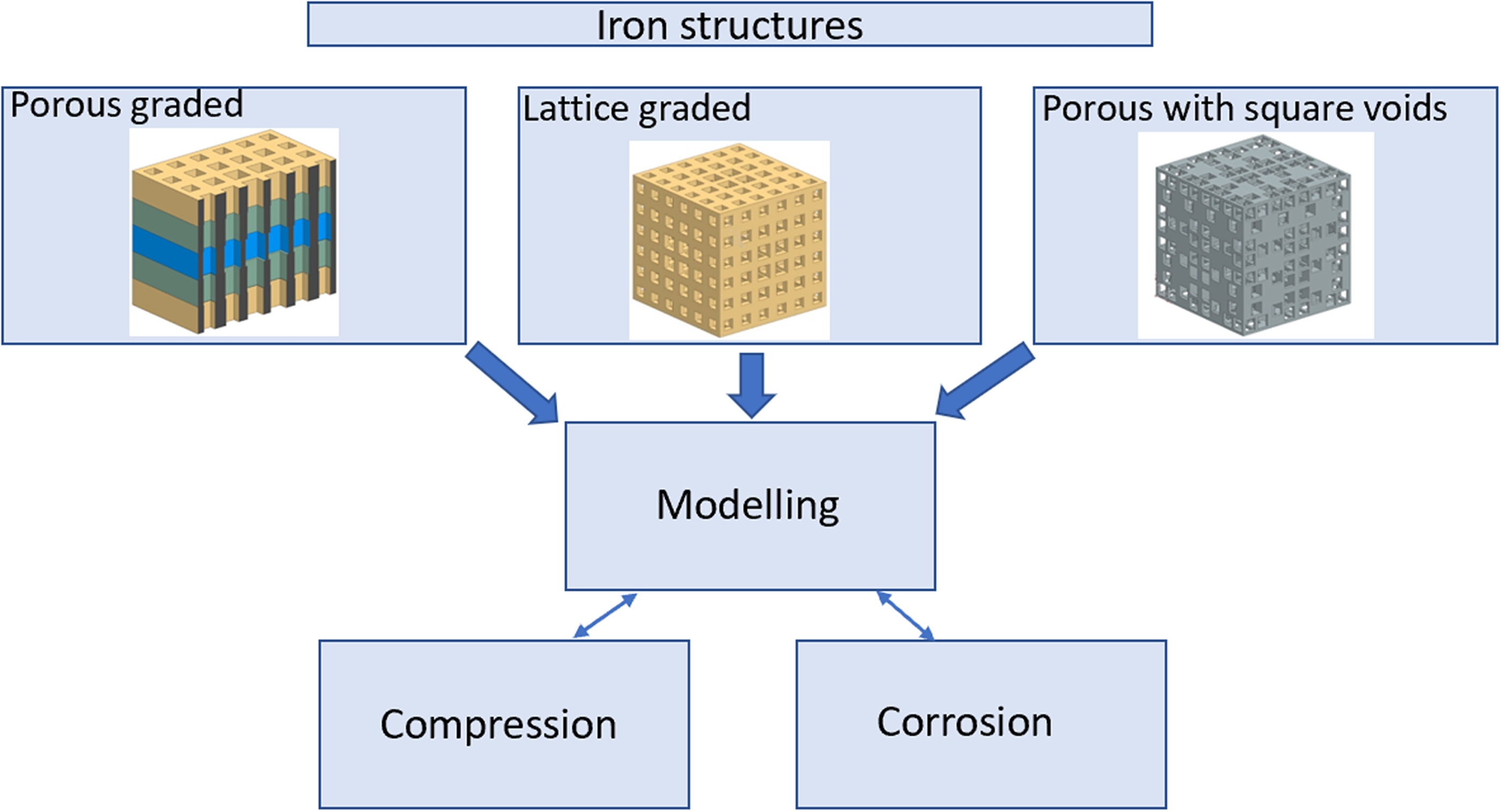
Schematic representation of the entire procedure of design and modelling of compression and degradation.

Architecture of the porous structures

The models of tailored porous structures can be combined into three sets, being the first two groups (a) and (b) designed with cell thickness variation, that is, they are graded structures. The three groups based on cubic cells are:

porous graded structures, which are obtained by the stacking of layers with square voids, along the z-axis (Figure 2), comprising samples G1 to G4;

lattice graded structures, which are truss-lattices with cubic shape in all three axes (Figure 3), consisting of samples G5 to G9;

porous structures with square voids, inspired by Hilbert fractal curves,³⁷ where the decomposition of the curves allows creating a ‘sort of random’ void distribution (Figure 4), including structures G10 to G12.

Figure 2.

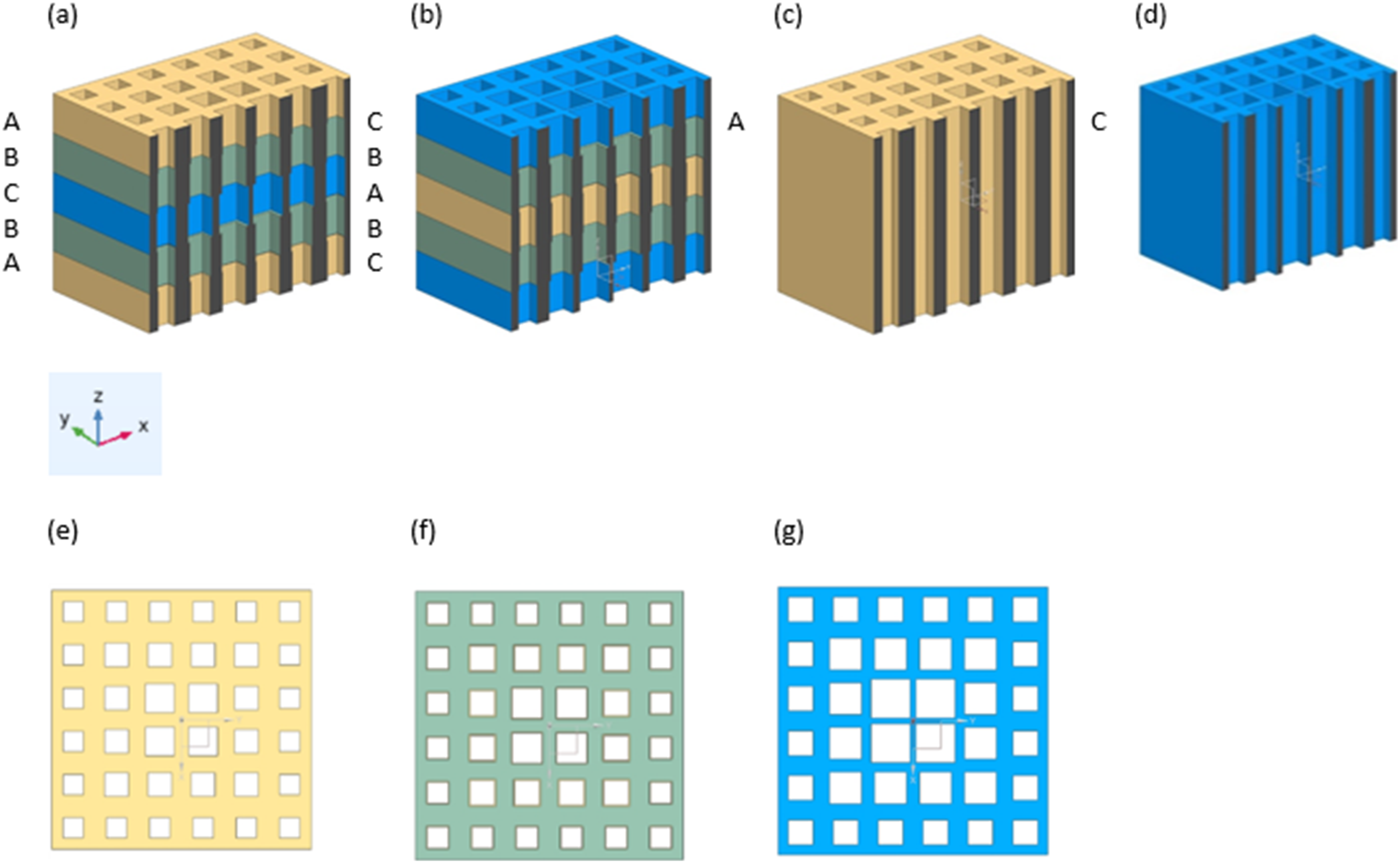
Schematic representation of the porous graded structures obtained by the stacking of layers with square voids. (a) G1, (b) G2, (c) G3 and (d) G4. Schematic representation of the stacked layers used: (e) plane A, (f) plane B, and (g) plane C.

Figure 3.

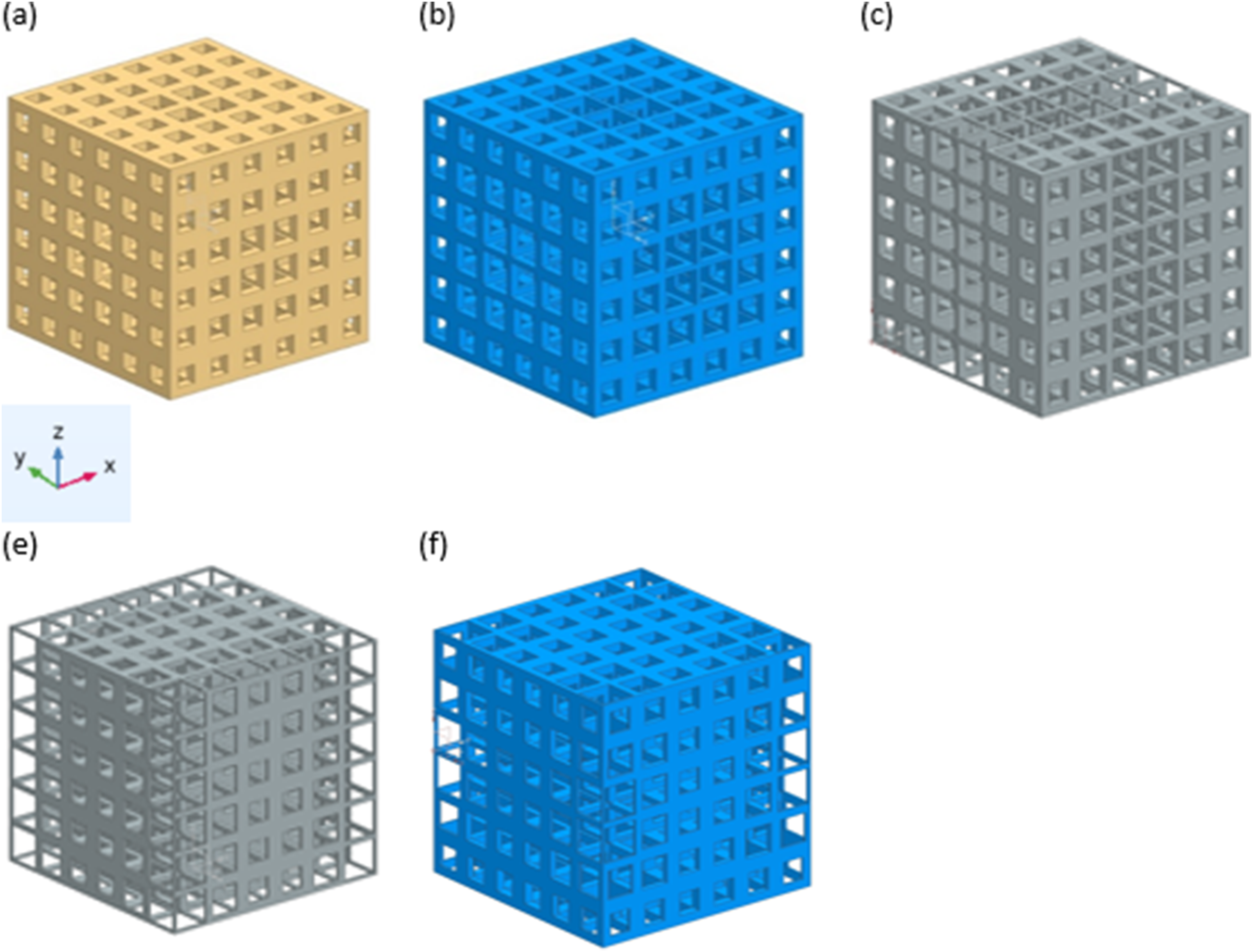
Graded lattice structures with cubic shape: (a) G5, (b) G6, (c) G7, (d) G8 and (e) G9.

Figure 4.

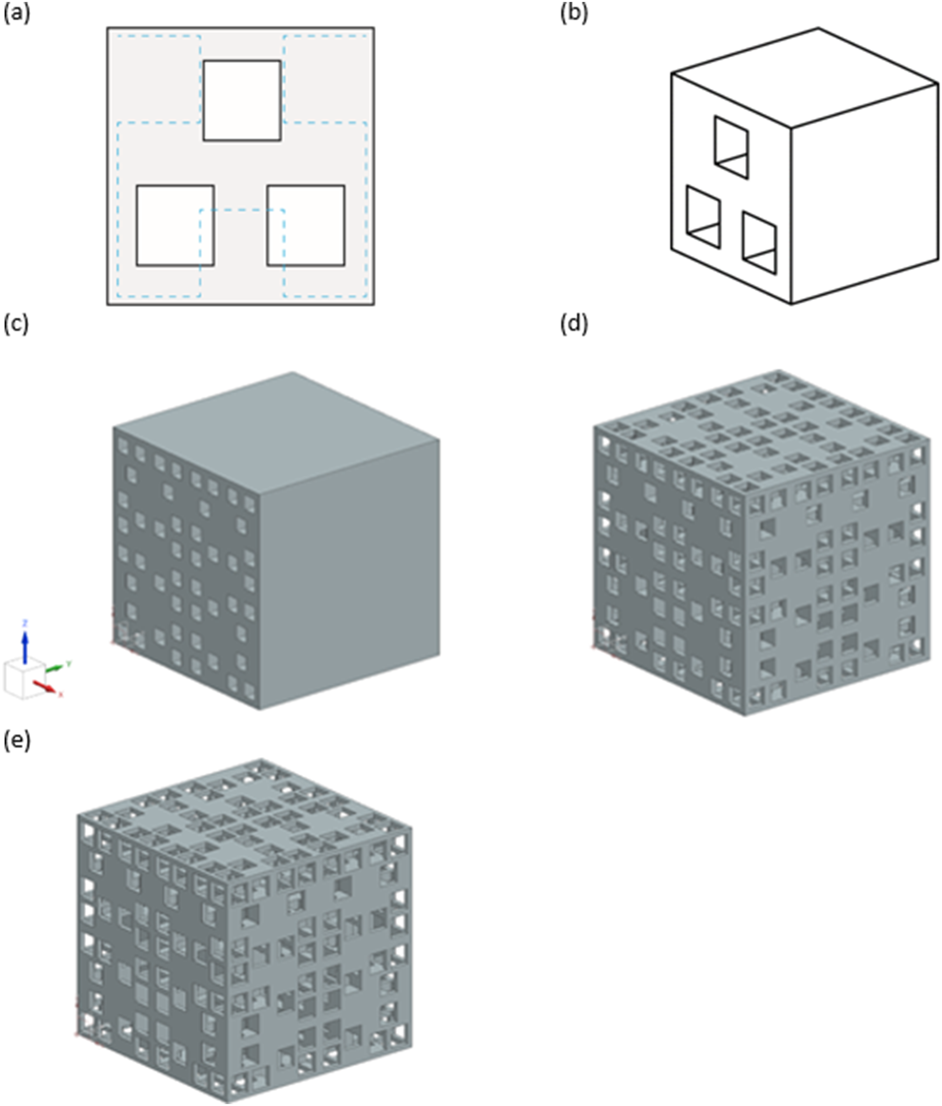
Porous structures inspired in Hilbert lines: (a) top plane, (b) unit cell, (c) G10, (d) G11 and (e) G12.

All structures studied have a symmetric distribution of cells, some with pores along one axis or others along the three axes.

In the first group, the stacking of layers consist of arrangements of five layers, each with 4 mm height and different variations of cell thickness (Figure 2). Each layer has four larger cells at the center, which are surrounded by 10 intermediate size cells, bounded by 20 smaller cells. Three different layers, A, B and C were considered (Figure 2(e) to (g)), with dimensions of voids given in Table 1. The structure denoted by G1 has a stacking sequence of A, B, C, B, A, while G2 follows the order C, B, A, B, C (Figure 2(a) and (b)). Structures G3 and G4 are one-dimensional extruded, only composed by layers A or layers C, respectively (Figure 2(c) and (d)).

Table 1.

Void dimensions of different layers.

Layer designation	Larger (mm)	Intermediate (mm)	Smaller (mm)
A	2.68	2.20	1.88
B	2.84	2.44	2.04
C	3.48	2.84	2.20

Lattice structures, from the second group, contain repeating unit cells with a cubic shape, a choice driven by results from a previous work.⁹ Lattices graded G5 to G9 present a symmetric cell distribution in all three axes, with all faces of the structures having the same arrangement. For example, each face of G5 has the cellular distribution of layer A, while G6 shows faces like layer C (Figure 3(a) and (b)). On structure G7, the smaller, intermediate and larger cells have the same dimensions as the ones of layer C. However, the cell distribution per face is different with a shell of 12 larger cells, with six intermediate cells on each side of the inner shell, plus two shells of six smaller cells. G8 and G9 structures are different combinations of cells with the same dimensions of G6, with the characteristic of having smaller cells in the center of the structure.

The design of the structures inspired by the Hilbert curves, G10 to G12, was obtained by adapting the Hilbert fractal curves, where straight lines were decomposed, as exemplified in Figure 4(a). The dashed line of Figure 4(a) represents a second-order Hilbert curve, which inspired the present authors in creating such geometry, with three holes. To account for a feasible manufacturability, the contour of the curve was not strictly followed, the holes being placed inside the unit cell (Figure 4(b)). The porous structure was constructed using repetitions of the unit cell (Figure 4(b)), with translations and rotations, giving rise to a ‘sort of random’ distribution of holes (Figure 4(c) to (e)). Sample G10 has a structure where the pores run along one axis, while G11 and G12 have the same cell distribution in all faces. Differences between samples G11 and G12 are only related to the two sizes of the voids.

In this type of models it is important to evaluate the relative density $\bar{ρ}$ , that is, the ratio of the cellular material density divided by the density of the cell wall compact material.³⁸ As in previous works,⁹ the relative density was measured by the CAD software (Siemens NX, Siemens Digital Industries Software), by calculating the ratio of the volume occupied by the solid divided by the volume of the rectangular cuboid that circumscribes it.

Table 2 presents some characteristics of the arrangements, such as the external dimensions, the relative density, the cross-section area and the surface area of the entire sample.

Table 2.

Characteristics of the structures.

Designations	Dimensions (mm)	Relative density	Cross-section area (mm²)	Surface area (mm²)
G1	24 × 24 × 20	0.68	576	9395
G2	24 × 24 × 20	0.65	576	12,395
G3	24 × 24 × 20	0.73	576	8735
G4	24 × 24 × 20	0.58	576	9948
G5	24 × 24 × 24	0.56	576	12,804
G6	24 × 24 × 24	0.34	576	11,388
G7	24 × 24 × 24	0.23	576	9840
G8	24 × 24 × 24	0.23	576	9840
G9	24 × 24 × 24	0.59	576	20,932
G10	16 × 16 × 16	0.78	256	4759
G11	16 × 16 × 16	0.41	256	6205
G12	16 × 16 × 16	0.30	256	5613

FE modelling of compression

The simulations of compression of the porous structures were performed using NX Nastran (version 2019.1) and Siemens NX as the pre and post-processor. Simulations were performed using the non-linear static solver (SOL 106 in NX).

All structures were modelled as pure iron, with properties of density, Poisson's ratio, elastic limit stress and Young's modulus, respectively, as ρ = 7874 kg/m³, ν = 0.29, σ_el = 150 MPa and E = 200 GPa.³⁹

Structures were meshed automatically by the software using different elements namely, tetrahedral, pyramidal and hexahedral elements (CTETRA10, CPYRAM and CHEXA8 in NX Nastran, respectively). The software generates the mesh by using hexahedral elements for larger, more regular volumes of solid, while for smaller, less regular volumes, tetrahedral elements are selected. The pyramidal elements perform the transition between the tetrahedral and the hexahedral elements. The tetrahedra are second-order elements, while the other two elements are of first order. The use of the combination of three types of elements aims to save computational resources. A benchmark was run on one geometry, first using a mesh combining all three types of elements and then using a mesh with only second-order tetrahedra. The first mesh had 320,050 nodes and the simulation took 6181 s (1 h 43 min, approximately) to finish while the second mesh had 1,042,811 nodes and took 35,502 s (9 h 51 min, approximately) to finish. In the end, the results were similar and thus the mixed mesh was used for the structural analyses that followed.

Compression simulations were performed imposing two boundary conditions: a fixed constraint on one end of the sample and an imposed displacement on the opposite end. In some cases, structures were simulated with only one quarter of the geometry in order to save computational resources by taking advantage of the symmetry of the structures.

The maximum imposed displacement was calculated for each sample height, in order to achieve a strain equal to 0.024, for all samples.

The results from the compression simulations include the load, which was calculated from the reaction force on the fixed end of the sample, as well as the longitudinal displacement. From the load–displacement curves, it is possible to assess, from the elastic zone, the absorbed energy, E_a, and the stiffness, K, respectively, from the area under the curve until a fixed displacement and from the slope of the curve.

The stress–strain plot was also constructed, for each case. The stress $σ = F / A_{c}$ , was calculated as the ratio between the load and the cross-sectional area, A_c, of the parallelepiped that circumscribes the structure. The strain, $ε = d l / l,$ was determined from the longitudinal displacement $d l$ divided by the sample height, l. The elastic limit stress, $σ_{e l}$ was also assessed from the stress–strain curve. In order to compare results from different structures with different space filling characteristics, the results were scaled by the relative density.

An evaluation of the structures’ strength was firstly performed by looking at the maximum von Mises stress, $σ_{m a x}$ , taken directly from NX Nastran. On a second approach and to further investigate the maximum strength, sub-modelling techniques were used to determine an upper bound of the stress concentration factor for each of the three sub-type of the porous structures, namely porous graded, lattices graded and Hilbert-inspired. The upper bound of the stress concentration factor is calculated for each sample of the three types of porous structures that presents the highest von Mises stresses and is then used for all others of each type.

Mesh convergence studies were undertaken. The convergence criterion was set as less than 2% changes in the highest von Mises stress. A range of element sizes varying from 0.5 to 1.25 mm was tested, being the element size of 0.75 mm the one chosen for the simulations. An example of the convergence study is given in Table 3, for the G5 structure.

Table 3.

Example of the convergence study for structure G5.

Element size (mm)	Number of elements	Maximum von Mises stress $σ_{m a x}$ (MPa)
1.25	39,027	138.4
1	51,618	141.4
0.75	98,409	142.8
0.5	260,418	139.6

Simulations of immersion degradation tests in SBF

It is known that the iron degradation mechanism stands on its electrochemical dissolution. The equations that rule the process are given in a previous publication.⁷

Corrosion simulations with the FE method were conducted using the software COMSOL Multiphysics version 5.6, with the Corrosion Module, as in previous works.^9,40 The conditions selected were the ones that enable the best fitting between numerical and experimental results.⁴⁰ The options provided to the software were: 3D dimensions, deformed geometry, secondary current distribution, average current density boundary condition (constant current density in the bulk surfaces).⁹ The polarization curve was obtained from the work of Sharma and Pandey.⁴¹ Among the several meshes, the mesh selected was the one referred to as finer (7), with element sizes between 0.14 and 1.93 mm.⁴² In summary, the options and the parameters used in the simulations with COMSOL, obtained previously⁴⁰ are indicated in Table 4.

Table 4.

Selected options and parameters used at the simulations with COMSOL, obtained from P.Neves.⁴⁰

Designations	Selection
Current distribution type	Secondary
Electrolyte	Simulated body fluid
Material	Pure Iron (99.8% purity)
Average current density	0.0523 A/m²
Temperature	37°C = 310.15 K
External electric potential	−0.57 V
Electrolyte conductivity	1.883 S/m

The porous structures were subjected to immersion tests in SBF at 37 °C. The container has a spherical shape with a radius of 100 mm. The sample was inserted in the center in order to avoid contact with the container walls (Figure 5).

Figure 5.

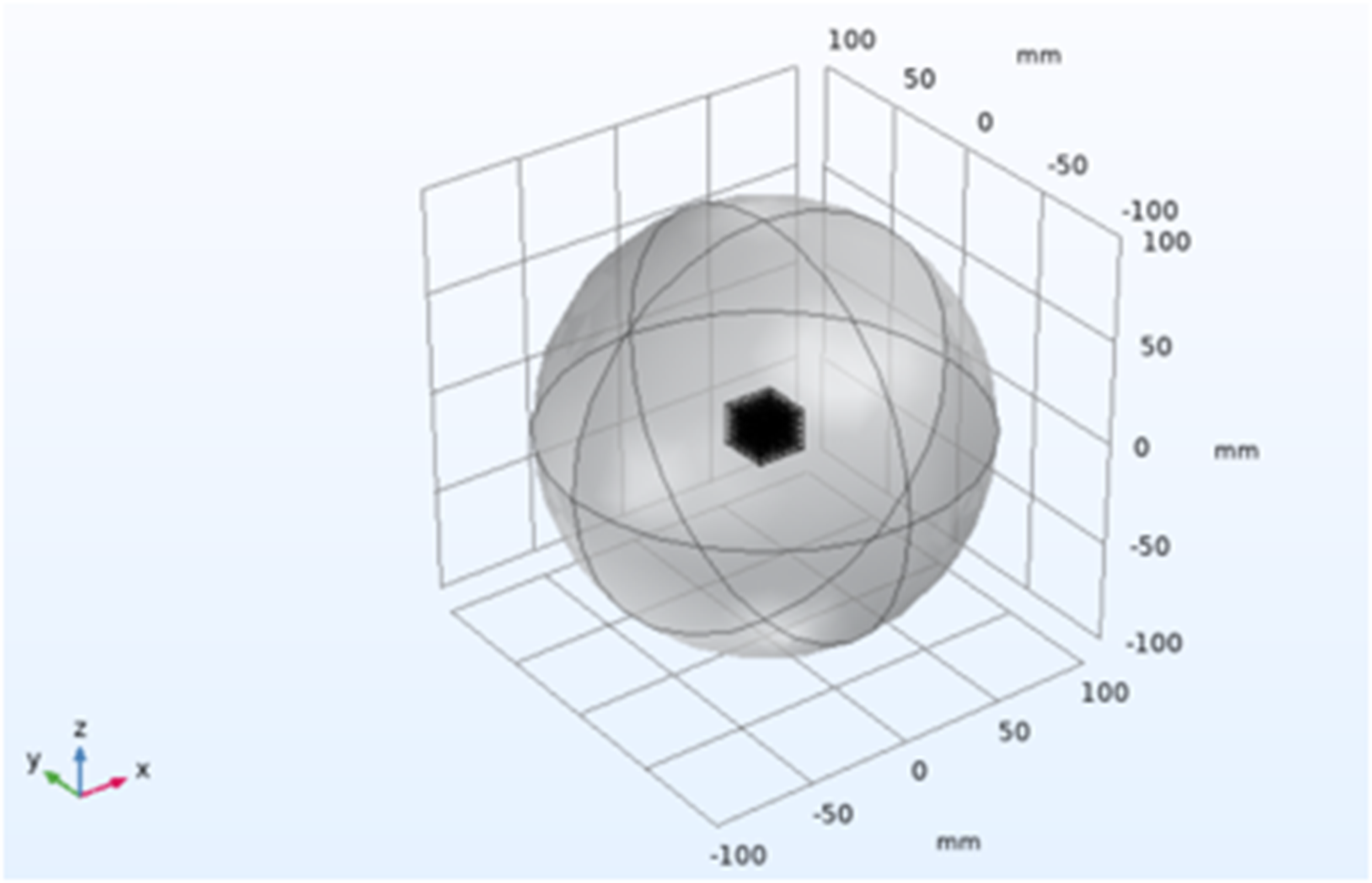
Schematic of the COMSOL module of corrosion: the iron sample is immersed in a simulated body fluid. The container has a spherical shape with a radius of 100 mm.

All simulations were performed until a minimum period of 28 days. The maximum duration of the simulations was related to the time at which the software stopped working, due to large decreases in the thickness of the cell walls, creating instabilities.

Being m₀ the initial mass and Δm the mass change at a certain time, it is possible to calculate the mass loss percentage, Δm/m₀ (%). The average immersion corrosion rate CR (mm/year) was determined from the mass loss values, according to ASTM standard G31–72,⁴³ as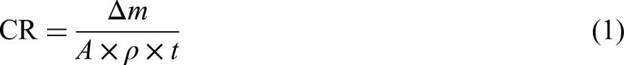

CR = \frac{Δ m}{A \times ρ \times t}

(1)

where A is the surface area of the samples (cm²), ρ is the theoretical density of iron (7.874 g/cm³), and t is the duration of the immersion test (year). The surface area (Table 2) was retrieved from the CAD software used to model the structures.

Results and discussion

Compression modelling

The current work studies three types of porous structures with variations of the relative density and different architectures or distribution of pores, for cubic shape cells.

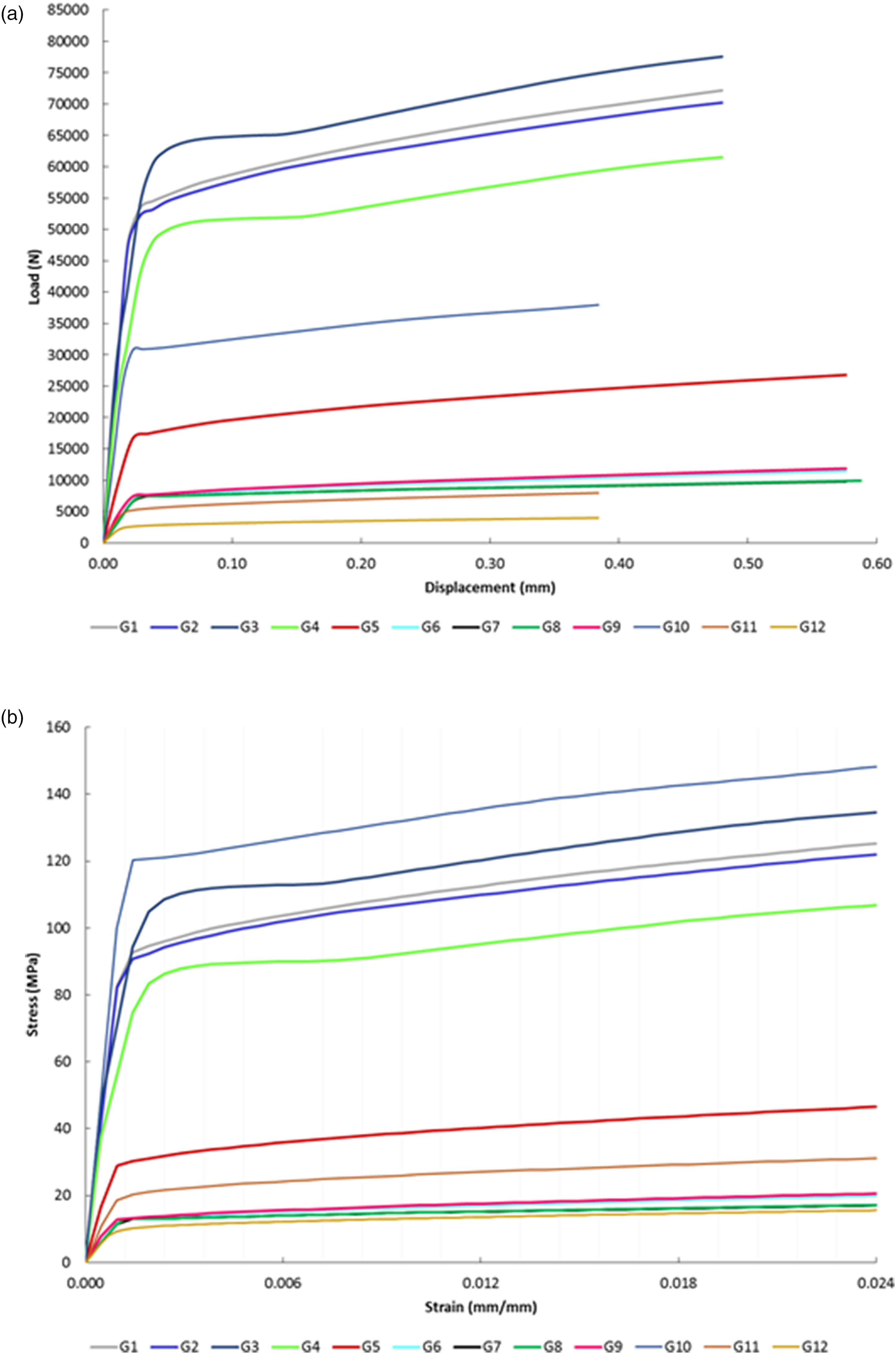
Figure 6 shows the compression load–displacement curves and their corresponding stress–strain curves for all porous structures. All stress–strain curves exhibit a linear elastic region until the elastic limit stress, $σ_{e l}$ , after which there is a second region with a lower slope.

Figure 6.

Results for compression of all structures: (a) load–displacement and (b) stress–strain curves.

Table 5 shows the FE results for compression tests of all porous structures, namely maximum von Mises stress $σ_{m a x}$ , stiffness K, and absorbed energy E_a, until a strain of 0.024 mm, and elastic limit stress, $σ_{e l}$ (scaled with the relative density, $\bar{ρ}$ ).

Table 5.

Fe results for compression tests of porous structures: maximum von Mises stress $σ_{m a x}$ , stiffness K, and absorbed energy E_a, until strain of 0.024, and elastic limit stress, $σ_{e l}$ (scaled with the relative density, $\bar{ρ}$ ).

Model	$\bar{ρ}$	$σ_{m a x} / \bar{ρ}$ (MPa)	$K / \bar{ρ}$ (KN/mm)	$E_{a} / \bar{ρ}$ (J)	$σ_{e l} / \bar{ρ}$
G1	0.68	456	3656	0.674	135
G2	0.65	405	3793	0.699	140
G3	0.73	349	2915	0.537	129
G4	0.58	443	2909	0.536	143
G5	0.56	568	1295	0.342	52
G6	0.34	1024	932	0.246	38
G7	0.23	1000	1247	0.330	52
G8	0.23	1500	1256	0.332	57
G9	0.59	627	547	0.145	22
G10	0.78	369	1716	0.454	154
G11	0.41	1305	554	0.146	46
G12	0.30	1440	379	0.100	30

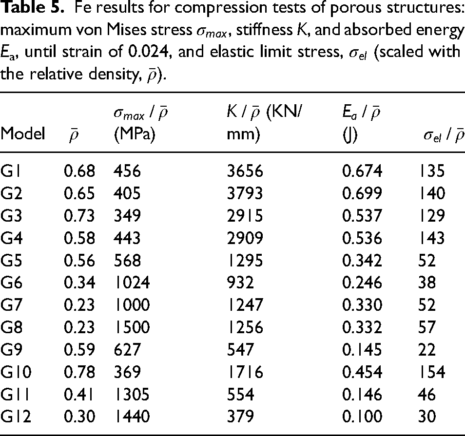
The porous structures G8, G11 and G12 possess the highest scaled von Mises stress, while G3 and G10 geometries have the lowest values of $σ_{m a x} / ρ$ . Porous structure G2 provides the highest stiffness and a bar over the density absorbed energy, while G12 presents the lowest values of such parameters. The highest scaled elastic limit stress was obtained with G2, G4 and G10, while the lowest values of $σ_{e l}$ were achieved in structures G9 and G12. Results indicate that among the several types of structures studied, namely porous graded (G1–G4), lattice graded (G5–G9) and Hilbert inspired (G10–G12), there is not a unique group of structures that prevails in terms of strength, stiffness, absorbed energy and elastic limit.

Figure 7 displays the von Mises stress distribution after an imposed displacement that corresponds to a strain of 0.024, for all structures. It is essential to look at the stress distributions that give information on the further deformation or eventually failure zones. A detailed look at the location of the maximum von Mises stress for four selected porous samples, G1, G4, G5 and G12, is exemplified in Figure 8. 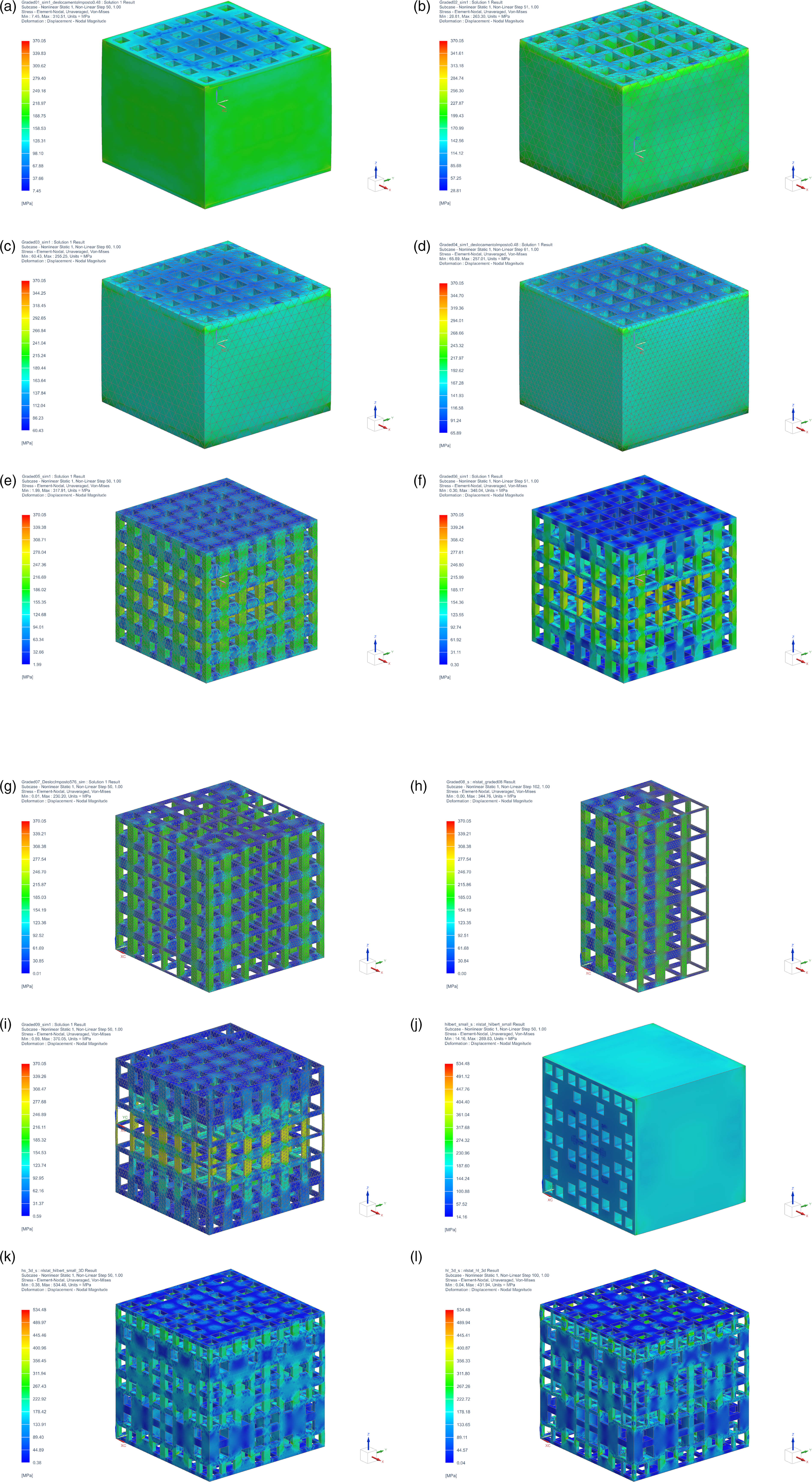The maximum von Mises stress, $σ_{m a x}$ , is located in the middle of the sample (Figure 8(a), (b), (e) and (f)), for specimens G1, G5, G6 and G9. On samples G2, G3, G4 and G10, $σ_{m a x}$ is found at, or near, the sample vertex (Figure 8(c) and (d)), while structures G7, G8, G11 and G12 present higher stress values near their external surfaces (Figure 8(g) and (h)).

Figure 7.

von Mises stress distribution after an imposed displacement, dl: (a) G1, dl = 0.48 mm; (b) G2, dl = 0.48 mm; (c) G3, dl = 0.48 mm; (d) G4, dl = 0.48 mm; (e) G5, dl = 0.58 mm; (f) G6, dl = 0.58 mm; (g) G7, dl = 0.58 mm; (h) G8, dl = 0.58 mm; (i) G9, dl = 0.58 mm; (j) G10, dl = 0.38 mm; (k) G11, dl = 0.38 mm; (l) G12, dl = 0.38 mm. The imposed displacements are different in order to obtain the same strain, due to the difference in the dimensions of samples. For G8, only a quarter of the structure was modelled.

Figure 8.

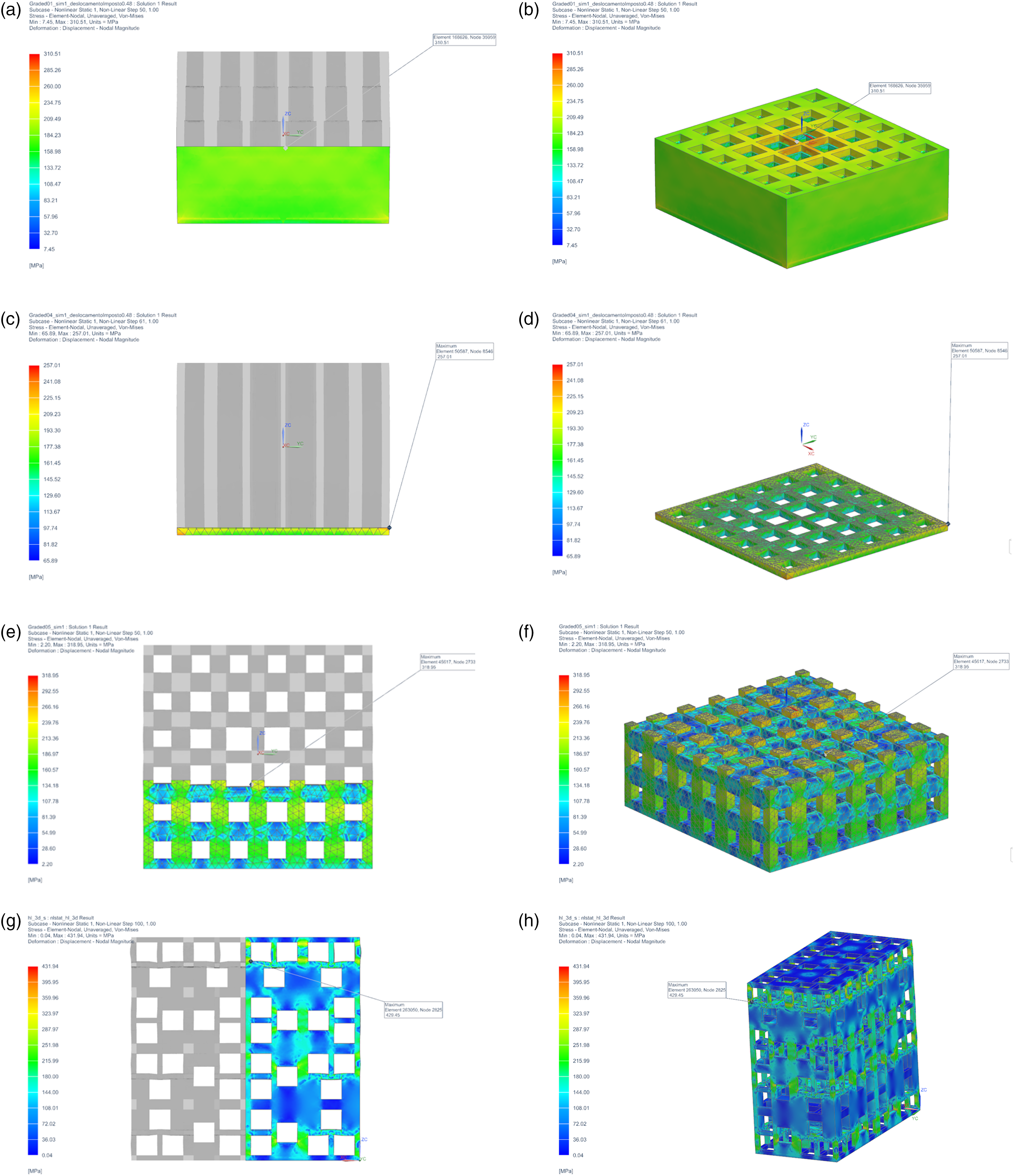
Examples of the location of the maximum von Mises stress after an imposed displacement. Two views of the cross-sections are displayed per sample: (a)(b) G1; (c)(d) G4; (e)(f) G5; (g)(h) G12.

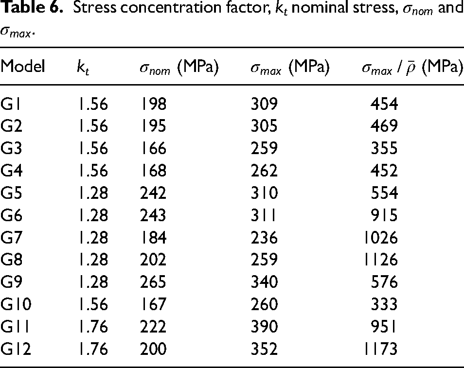
The sub-modelling technique was applied for samples G2, G9 and G11. A small piece of each structure is cut from the main model, from the region where the von Mises stress field registers the highest values, at which small details (corner filets) are added (Figure 9). The displacement field calculated in the analyses with the full structures is used as the only boundary condition. The upper bound of the maximum von Mises stress was estimated, along with an approximation for the nominal von Mises stress in that zone, leading to a value for the upper bound of the stress concentration factor, k_t. The values obtained for k_t of samples G2, G9 and G11, were respectively 1.56, 1.28 and 1.76. 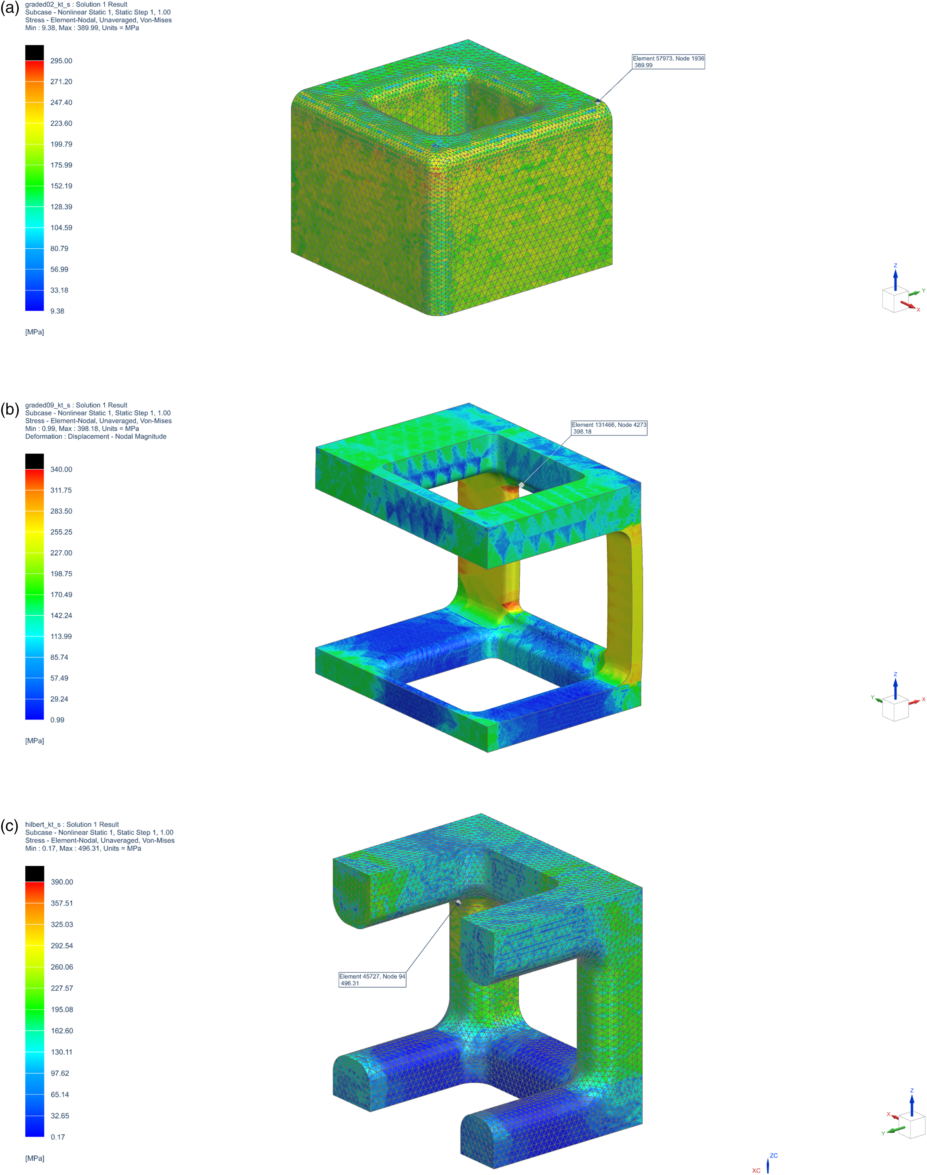After this, a nominal stress $σ_{n o m}$ was calculated for the entire sample without fillets. An estimation of the upper bound of the maximum von Mises stress $σ_{m a x}$ was made by multiplying the stress concentration factor by the nominal stress, as presented in Table 6. The values of the upper bound of the maximum von Mises stress $σ_{m a x},$ scaled with the relative density, are in general, lower than the previous ones presented in Table 5, in particular for samples which present the highest values.

Figure 9.

Localization of the von Mises maximum stress after applying a sub-modelling technique for (a)–(c) samples G2, G9 and G11, respectively.

Table 6.

Stress concentration factor, k_t nominal stress, $σ_{n o m}$ and $σ_{m a x}$ .

Model	k_t	$σ_{n o m}$ (MPa)	$σ_{m a x}$ (MPa)	$σ_{m a x} / \bar{ρ}$ (MPa)
G1	1.56	198	309	454
G2	1.56	195	305	469
G3	1.56	166	259	355
G4	1.56	168	262	452
G5	1.28	242	310	554
G6	1.28	243	311	915
G7	1.28	184	236	1026
G8	1.28	202	259	1126
G9	1.28	265	340	576
G10	1.56	167	260	333
G11	1.76	222	390	951
G12	1.76	200	352	1173

The compression properties of the porous materials are affected by their porosity, P, which could be defined as P = 1− $\bar{ρ}$ . Porous materials are designated as cellular materials if the relative density is around or lower than 0.3.³⁸ Authors defined that the elastic limit stress of open cellular regular hexagonal materials is scaled to the relative density with a slope of 3/2.³⁸ To compare with the theoretical predictions, the data of the elastic limit stress of all samples was plotted as a function of the relative density in Figure 10(a). A solid line with a slope of 3/2 was superimposed on the obtained data, indicating that it has a good correlation with the Gibson-Ashby model, although not all the structures are cellular solids, neither are they made of hexagonal cells. This means that the relative density has a strong effect on the elastic limit stress.

Figure 10.

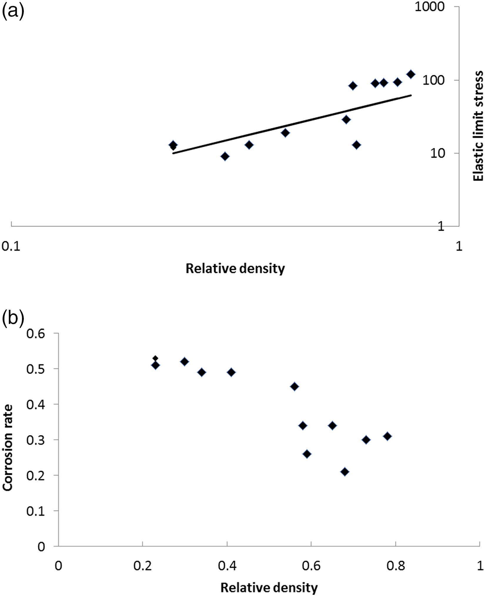
(a) Log–log plot of the yield stress as a function of the relative density. A solid line with a slope of 3/2 is superimposed to the obtained data; (b) corrosion rate as a function of the relative density.

Besides relative density, the arrangements of pores may have an influence on the mechanical properties of the porous structures. One of the purposes of the current work was to evaluate if a graded structure, for example with inner large and low-density cells surrounded by outer smaller and high-density cells (dense-out) could mimic the trabecular bone structure and attain suitable properties for bone substitutes. This was the case of porous graded structures (G1–G4) which were designed by stacking three planes with the mentioned graded structure. Although G1 and G2 have different stacking sequences, they exhibit the same elastic limit stress, probably because they have the same relative density. Samples G3 and G4 may be regarded as upper and lower bound values for type (a) structures, as they are made only of the highest and lowest density planes, respectively. Among the group (a), G4 is the one that presents the lowest value of $σ_{e l}$ , but the value is still very high, when compared with other geometries.

Group (b) includes lattice graded structures G5–G9, being each face of samples G5, G6 and G7 of the dense-out type, while each face of G8 and G9 is of the dense-in type.

Comparing the elastic limit stress of structures G4, G5 and G9, which have almost the same relative density, one concludes that G5 and G9 possess lower elastic limit stress due to their pore arrangement. Samples G6, G7, G8 and G9 attain the almost the same values of $σ_{e l}$ , despite the fact that they have different geometries and different relative densities, with the exception of G7 and G8.

Hilbert inspired geometries G11 and G12 present lower values of $σ_{e l}$ in comparison with G10, which has pores only in one direction.

The graded structures studied in the present work may not be directly compared with the ones currently available in the literature. For example, Li et al.,²³ only reported, for gradients in one plane, that a distribution with the presence of outer dense cells leads to a lower elastic limit stress in comparison with an inner dense cell configuration, being the former preferable to simulate bone.

Overall, the iron structures that present lower relative density and lower elastic limit stress are G6, G7, G8 and G12. It means that three lattice graded (G6, G7 and G8) and one more random pore distribution (G12) may be regarded as good choices to simulate trabecular bone substitutes.

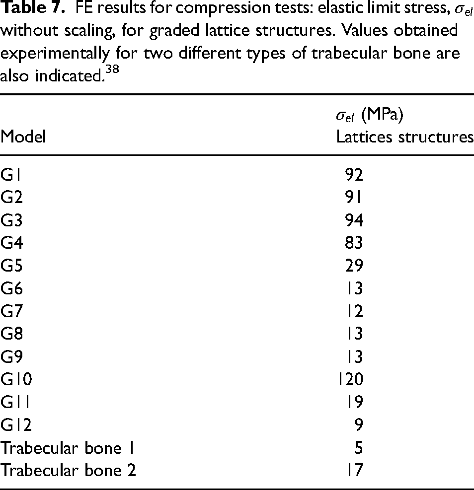
Bone properties depend on many factors, leading to a dispersion of values of the elastic limit stress of trabecular bone, that can vary in the range 0.2–80 MPa,⁴⁴ or around 5 and 17 MPa (Table 7).⁴⁵ From Table 7, one may conclude that samples G5–G9 and G11–G12 exhibit values of elastic limit from 9 to 29 MPa, thus falling in the range of human trabecular bone. The results obtained are comparable with previous results attained with iron non-graded structures that showed elastic limit stress in the range of 13–32 MPa⁹, or in the range of 4–22 MPa achieved by Sharma and Pandey.⁴⁶

Table 7.

FE results for compression tests: elastic limit stress, $σ_{e l}$ without scaling, for graded lattice structures. Values obtained experimentally for two different types of trabecular bone are also indicated.³⁸

Model	$σ_{e l}$ (MPa)Lattices structures
G1	92
G2	91
G3	94
G4	83
G5	29
G6	13
G7	12
G8	13
G9	13
G10	120
G11	19
G12	9
Trabecular bone 1	5
Trabecular bone 2	17

Corrosion modelling

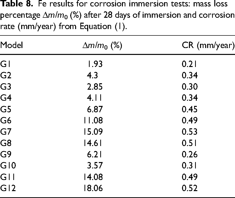
Figure 11(a) shows an image, obtained with COMSOL, of the iron structure G1 after immersion in SBF for 364 days, while Figure 11(b) displays a view of the top plane of the sample. A plot of the mass loss as a function of time is exhibited in Figure 11(c). Figure 12 presents images of all degraded iron samples at the maximum timespans of simulations. The timespan is not equal to all specimens, because on some structures it is not possible to go further, due to non-convergence problems caused by the thinning of struts. FE results for corrosion immersion tests expressed in mass loss percentage Δm/m₀ (%) after 28 days of immersion and corrosion rate (mm/year) from equation (1) are displayed in Table 8.

Figure 11.

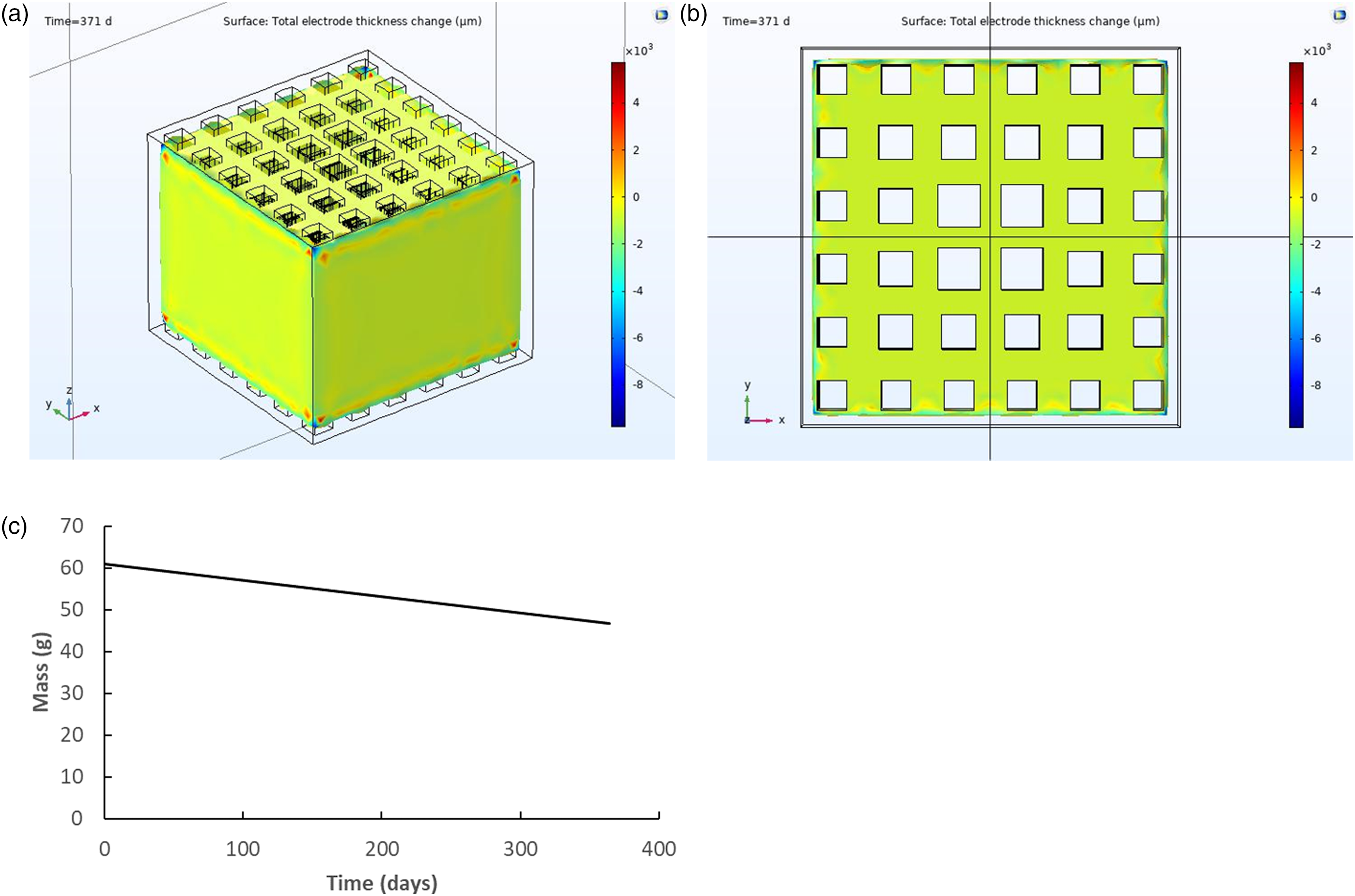
FE results for the corrosion of iron sample G1: (a) image of the degraded sample after 364 days of immersion; (b) view of top plane; (c) mass loss as a function of time.

Figure 12.

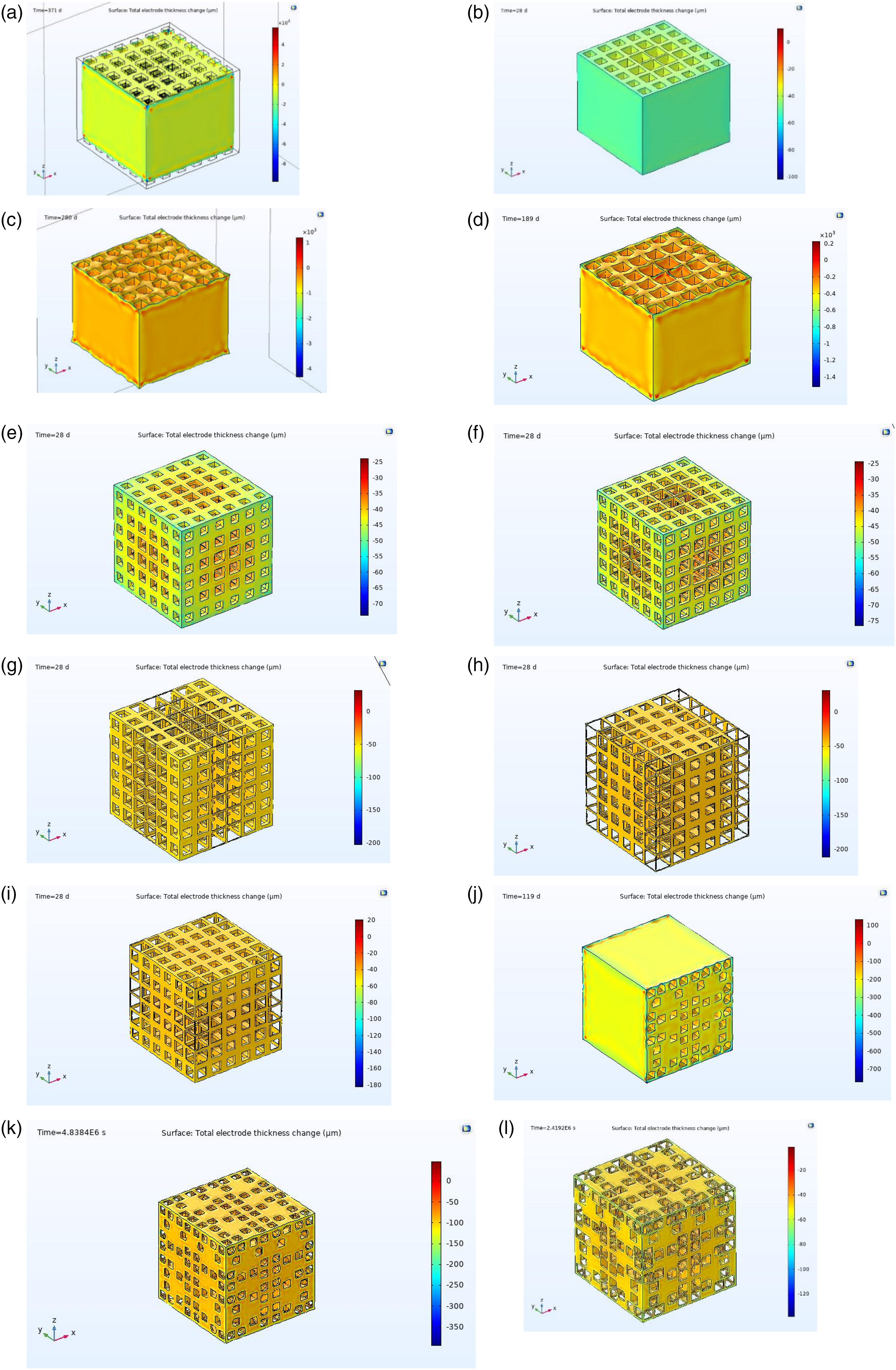
FE results for the corrosion of iron samples G1 to G12: (a)–(k) images after the maximum corrosion time simulated in days for (a) G1, t = 364 days; (b) G2, t = 28 days; (c) G3, t = 280 days; (d) G4, t = 190 days; (e) G5, t = 28 days; (f) G6, t = 28 days; (g) G7, t = 28 days; (h) G8, t = 28 days; (i) G9, t = 28 days; (j) G10, t = 120 days; (k) G11, t = 60 days; (l) G12, t = 28 days.

Table 8.

Fe results for corrosion immersion tests: mass loss percentage Δm/m₀ (%) after 28 days of immersion and corrosion rate (mm/year) from Equation (1).

Model	Δm/m₀ (%)	CR (mm/year)
G1	1.93	0.21
G2	4.3	0.34
G3	2.85	0.30
G4	4.11	0.34
G5	6.87	0.45
G6	11.08	0.49
G7	15.09	0.53
G8	14.61	0.51
G9	6.21	0.26
G10	3.57	0.31
G11	14.08	0.49
G12	18.06	0.52

The images of Figure 12 revealed that the degradation, that is, the change of thickness is more pronounced at the external surfaces and at the struts, which have an initial lower thickness. This is in agreement with the findings of Li et al.²³ that obtained a faster degradation of the struts of the border samples, while struts in the center remained almost intact. However, as stated above, the structures of the current works are not directly comparable with the geometries of such studies.²³

The relative density of the structures also seems to influence the degradation properties. Table 8 indicate that specimens with low relative density G6, G7, G8, G11 and G12 present the highest values of mass loss percentage and corrosion rate. This is in accordance with works that report that structures with high porosity exhibit high weight loss, showing high corrosion rates in comparison with lower porosity arrangements.^8,23 Figure 10(b) presents the corrosion rate as a function of the relative density. It is clear that structures with lower relative densities, that is, higher porosities tend to have higher corrosion rates.

The degradation dependence on geometry may be regarded as follows. In type (a) porous graded samples, specimens G1 and G2 possess almost the same relative density but different geometries, being the weight loss higher in G2, which has larger pores at the surface. Comparing G3 (type a) with G5 (type b) and G4 (type a) with G6 (type b), one can find that samples with pores along the three axes have faster thickness changes than specimens with pores in one direction only.

Samples G3 and G10 (type c) have almost the same relative density, but G10 with a sort of random pore distribution seems to degrade faster than a graded porous structure (G3).

Although G4, G5 and G9 have almost the same relative density and different geometry, their degradation rate is almost the same for the three specimens. It appears that the degradation mechanism is geometry-dependent, since different designs will allow for different pathways of fluid flow inside the porous structure.

The results obtained for the corrosion rate evaluated by the mass loss are in the range 2–18% (Table 8). Experimental data, from other authors, report that after immersion in SBF, porous iron shows a mass loss of 7%¹⁰ or of 5–16%,²³ which is the ideal degradation rate for bone replacement. The values of mass loss obtained for specimens G5–G9 and G11–G12 fall into that interval, except for sample G12 which presents a higher value of 18%.

The average immersion corrosion rate was found to be in the interval of 0.2–0.53 mm/year (Table 8). The values obtained are close to the corrosion rate indicated for ideal bone substitutes of 0.2–0.5 mm/year.⁴⁷

In summary, structures G6, G7, G8 and G12 that have low relative densities combine low elastic limit stress with large corrosion rates, presenting values that are adequate for bone replacement.

Conclusions

In the pursuit of adequate structures for iron biodegradable structures for bone replacement, several porous arrangements were studied. Bone substitutes should have a porous structure, to allow for cell activity associated with fluid flow and to reduce the stiffness avoiding or at least minimizing the stress-shielding effect.

Three groups of iron porous structures, in a total of 12 geometries, were designed and their mechanical and corrosion properties were evaluated by FE analysis.

Compression results showed that the properties of the iron porous structures were influenced by their relative density and geometry. These two factors also influence the degradation properties.

One may conclude that three lattices graded (G6, G7 and G8) and another structure with a more random pore distribution (G12) may be regarded as good choices as bone substitutes. Those structures have low relative densities combined with low elastic limit stress with large corrosion rates. They exhibit elastic limit stress close to the values for human trabecular bone and degradation rates close to the ideal values established for biodegradable implants.

The modelling study demonstrates that it is possible to match the iron properties to the ones required for biodegradable devices, by choosing adequate porous arrangements that tailor the mechanical and the corrosion behaviour.

Highlights

Porous iron structures to be used as bone biodegradable implants are studied.

Several types of porous structures are analysed, such as porous graded, lattice graded, and a sort of random distribution of pores.

FE analyses of uniaxial compression and of the corrosion of the porous structures were undertaken.

Low relative density structures present mechanical properties closer to the human bone.

Corrosion rates are adequate for use as bone temporary implants.

Footnotes

Acknowledgements

This work was supported by FCT, through IDMEC, under LAETA, Project UIDB/50022/2020, and FCT project PTDC/CTM-CTM-3354/2021. The authors also acknowledge the support given by the projects CQE-UIDB/00100/2020 and UIDB/50006/2020.

Declaration of conflicting interests

The author(s) declared no potential conflicts of interest with respect to the research, authorship, and/or publication of this article.

Funding

The author(s) disclosed receipt of the following financial support for the research, authorship, and/or publication of this article: This work was supported by the Fundação para a Ciência e a Tecnologia (grant number CQE-UIDB/00100/2020 and UIDB/50006/2020, projects UIDB/50022/2020, PTDC/CTM-CTM-3354/2021).

ORCID iDs

F Alves

L Reis

AM Deus

MB Silva

C Santos

MF Vaz

References

Zheng

Witte

. Biodegradable metals. Mater Sci Eng R Reports 2014; 77: 1–34.

Hermawan

. Updates on the research and development of absorbable metals for biomedical applications. Prog Biomater 2018; 7: 93–110.

Sansone

Pagani

Melato

. The effects on bone cells of metal ions released from orthopaedic implants. A review. Clin CASES Miner BONE Metab 2013; 10: 34–40.

Basri

Prakoso

Sulong

, et al. Mechanical degradation model of porous magnesium scaffolds under dynamic immersion. Proc IMechE Part L: J Materials: Design and Applications 2020; 234: 175–185.

Dong

Lin

Boccaccini

, et al. Corrosion behavior of biodegradable metals in two different simulated physiological solutions: comparison of Mg, Zn and Fe. Corros Sci 2021; 182: 109278.

Paiva

JCC

Oliveira

Vaz

, et al. Biodegradable bone implants as a new hope to reduce device-associated infections—A systematic review. Bioengineering 2022; 9: 409.

Salama

Vaz

Colaço

, et al. Biodegradable iron and porous iron: mechanical properties, degradation behaviour, manufacturing routes and biomedical applications. J Funct Biomater 2022; 13: 72.

Sharma

Pandey

. Corrosion rate modelling of biodegradable porous iron scaffold considering the effect of porosity and pore morphology. Mater Sci Eng C 2019; 103: 109776.

Salama

Alves

Reis

, et al. Finite element simulations of mechanical behaviour and degradation of iron lattices. Proc IMechE Part L: J Materials Design and Applications 2023: 237: 1379–1393.

10.

Putra

Leeflang

Minneboo

, et al. Extrusion-based 3D printed biodegradable porous iron. Acta Biomater 2021; 121: 741–756.

11.

Jahr

Lietaert

, et al. Additively manufactured biodegradable porous iron. Acta Biomater 2018; 77: 380–393.

12.

du Plessis

Yadroitsava

Yadroitsev

, et al. Numerical comparison of lattice unit cell designs for medical implants by additive manufacturing. Virtual Phys Prototyp 2018; 13: 266–281.

13.

Amani

Dancette

Delroisse

, et al. Compression behavior of lattice structures produced by selective laser melting: x-ray tomography based experimental and finite element approaches. Acta Mater 2018; 159: 395–407.

14.

, et al. Design and performance evaluation of additively manufactured composite lattice structures of commercially pure Ti (CP–Ti). Bioact Mater 2021; 6: 1215–1222.

15.

Chatzigeorgiou

Piotrowski

Chemisky

, et al. Numerical investigation of the effective mechanical properties and local stress distributions of TPMS-based and strut-based lattices for biomedical applications. J Mech Behav Biomed Mater 2022; 126: 105025.

16.

Yang

Huang

Song

. Constructing lattices with graded features in spatial distribution for tissue engineering. Mater Lett 2022; 311: 131609.

17.

Md Yusop

Al Sakkaf

Nur

Modifications on porous absorbable Fe-based scaffolds for bone applications: a review from corrosion and biocompatibility viewpoints. J Biomed Mater Res Part B Appl Biomater 2022; 110: 18–44.

18.

Feng

Hao

, et al. A review on functionally graded materials and structures via additive manufacturing: from multi-scale design to Versatile functional properties. Adv Mater Technol 2020; 5: 1900981.

19.

Zhang

X-Y

Fang

Leeflang

, et al. Topological design, permeability and mechanical behavior of additively manufactured functionally graded porous metallic biomaterials. Acta Biomater 2019; 84: 437–452.

20.

Al-Ketan

Lee

D-W

Rowshan

, et al. Functionally graded and multi-morphology sheet TPMS lattices: design, manufacturing, and mechanical properties. J Mech Behav Biomed Mater 2020; 102: 103520.

21.

Maskery

Aboulkhair

Aremu

, et al. A mechanical property evaluation of graded density Al-Si10-Mg lattice structures manufactured by selective laser melting. Mater Sci Eng A 2016; 670: 264–274.

22.

Garrido Silva

Alves

Sardinha

, et al. Functionally graded cellular cores of sandwich panels fabricated by additive manufacturing. Proc IMechE Part L: J Material Design and Applications 2022; 236: 1814–1828.

23.

Jahr

Pavanram

, et al. Additively manufactured functionally graded biodegradable porous iron. Acta Biomater 2019; 96: 646–661.

24.

Xiao

Song

. Additively-manufactured functionally graded Ti-6Al-4V lattice structures with high strength under static and dynamic loading: experiments. Int J Impact Eng 2018; 111: 255–272.

25.

Niknam

Akbarzadeh

. Graded lattice structures: simultaneous enhancement in stiffness and energy absorption. Mater Des 2020; 196: 109129.

26.

Choy

Sun

C-N

Leong

, et al. Compressive properties of functionally graded lattice structures manufactured by selective laser melting. Mater Des 2017; 131: 112–120.

27.

Efremov

Martínez

Lefebvre

. 3D periodic cellular materials with tailored symmetry and implicit grading. Comput Des 2021; 140: 103086.

28.

Han

Wang

, et al. Continuous functionally graded porous titanium scaffolds manufactured by selective laser melting for bone implants. J Mech Behav Biomed Mater 2018; 80: 119–127.

29.

Limmahakhun

Oloyede

Sitthiseripratip

, et al. Stiffness and strength tailoring of cobalt chromium graded cellular structures for stress-shielding reduction. Mater Des 2017; 114: 633–641.

30.

Yang

Mertens

Ferrucci

, et al. Continuous graded gyroid cellular structures fabricated by selective laser melting: design, manufacturing and mechanical properties. Mater Des 2019; 162: 394–404.

31.

Liang

Yang

Xie

, et al. Trabecular-like Ti-6Al-4V scaffolds for orthopedic: fabrication by selective laser melting and in vitro biocompatibility. J Mater Sci Technol 2019; 35: 1284–1297.

32.

Murr

Gaytan

Medina

, et al. Next-generation biomedical implants using additive manufacturing of complex, cellular and functional mesh arrays. Philos Trans R Soc A Math Phys Eng Sci 2010; 368: 1999–2032.

33.

Zhou

Jin

. Functionally graded scaffolds with programmable pore size distribution based on triply periodic minimal surface fabricated by selective laser melting. Materials (Basel) 2020; 13: 5046.

34.

Nguyen

CHP

Kim

Choi

. Design for additive manufacturing of functionally graded lattice structures: a design method with process induced anisotropy consideration. Int J Precis Eng Manuf Technol 2021; 8: 29–45.

35.

Yang

Chen

Sun

, et al. Compressive properties of bidirectionally graded lattice structures. Mater Des 2022; 218: 110683.

36.

Avchukir

Burkitbayeva

. Conductive polymer/SiO2 composite as an anticorrosive coating against carbon dioxide corrosion of mild steel. A simulation study. Eurasian Chem J 2020; 22: 295.

37.

Martínez-Magallanes

Cuan-Urquizo

Crespo-Sánchez

, et al. Hierarchical and fractal structured materials: design, additive manufacturing and mechanical properties. Proc IMechE Part L: J Material Design and Applications 2023: 237: 650–666.

38.

Gibson

Ashby

. Cellular solids: structure and properties. 2nd ed. Cambridge: Cambridge University Press, 1997.

39.

Al Baida

Langlade

Kermouche

, et al. Identifying the stress–strain curve of materials by microimpact testing. Application on pure copper, pure iron, and aluminum alloy 6061-T651. J Mater Res 2015; 30: 2222–2230.

40.

Neves

. Finite element modelling of iron corrosion behavior . Master Thesis, Universidade de Lisboa, Instituto Superior Técnico, 2021.

41.

Sharma

Pandey

. Corrosion behaviour of the porous iron scaffold in simulated body fluid for biodegradable implant application. Mater Sci Eng C 2019; 99: 838–852.

42.

Comsol Software for Multiphysics Simulation: Corrosion Module, https://www.comsol.com.

43.

ASTM G31-72. Standard Practice For Laboratory Immersion Corrosion Testing For Metals. ASTM Int. Epub ahead of print 2004. DOI: 10.1520/G0031-72R04.

44.

Keaveny

Morgan

Niebur

, et al. Biomechanics of trabecular bone. Annu Rev Biomed Eng 2001; 3: 307–333.

45.

Ghouse

Reznikov

Boughton

, et al. The design and in vivo testing of a locally stiffness-matched porous scaffold. Appl Mater Today 2019; 15: 377–388.

46.

Sharma

Pandey

. Morphological and mechanical characterization of topologically ordered open cell porous iron foam fabricated using 3D printing and pressureless microwave sintering. Mater Des 2018; 160: 442–454.

47.

Gao

Yao

, et al. Highly biodegradable and bioactive Fe-Pd-bredigite biocomposites prepared by selective laser melting. J Adv Res 2019; 20: 91–104.

Mechanical and corrosion performance of biodegradable iron porous structures

Abstract

Keywords

Introduction

Materials and methods

Architecture of the porous structures

FE modelling of compression

Simulations of immersion degradation tests in SBF

Results and discussion

Compression modelling

Corrosion modelling

Conclusions

Highlights

Footnotes

Acknowledgements

Declaration of conflicting interests

Funding

ORCID iDs

References