Sage Journals: Discover world-class research

Abstract

This study presents a dynamic analysis for a model of a suspended cable subjected to both static and dynamic loading conditions. To enhance stability and reduce undesired vibrations, particularly in the resonance region, the nonlinear integral positive position feedback controller with time delay (NIPPFC) is implemented. The differential equation (DE) for a hung cable is developed using the Hamilton variation approach (HVA) and solved by the multiple-scales approach (MSA) in to appropriate order to get the approximate solutions (AS). By comparing the AS to the determined numerical solutions (NS) using the Runge–Kutta method of fourth order (RK-4), the accuracy of the AS is confirmed. The modulation equations (ME) are obtained by exploring solvability criteria and resonance instances. Graphical representations of the time histories and frequency responses of the derived solutions are presented using MATLAB software and Wolfram Mathematica 13.2. Additionally, a graphical analysis is performed on the temporal histories of the achieved solutions, both with and without control. Resonance curves are also utilized to explore stability analysis and steady-state solutions. Furthermore, the model’s nonlinear dynamics are investigated through bifurcation analysis and visualized using bifurcation diagrams to identify critical parameters leading to qualitative changes in system behavior. The Poincaré map is utilized to study periodic and chaotic oscillations, providing insights into the system’s long-term stability and the emergence of chaotic dynamics. The significance of the acquired results lies in their contribution to understanding and mitigating dynamic instabilities and chaotic behavior in flexible structures under varying operational conditions. Furthermore, a comparative analysis with conventional controllers, such as the linear negative displacement feedback controller (LDFC), linear negative velocity feedback controller (LVFC), and negative cubic velocity feedback controller (CVFC), showed that the NIPPFC significantly enhances damping. The amplitude of $q (τ)$ was reduced up to 99.44%, with the best result achieved at time delay $T = 0.004$ . This model is widely applied in the analysis and design of flexible structures such as suspension bridges, transmission lines, and cable-supported systems. In addition, it helps engineers analyze how structures respond to static and dynamic forces, such as weight, wind, earthquakes, or moving loads. By monitoring displacements, it predicts critical behaviors like vibrations, deflections, or resonance, preventing structural instability or failure. It also aids in vibration control and optimization to improve safety and performance.

Keywords

positive position feedback controller multiple scale algorithm bifurcation analysis stability Poincare’ maps dynamical system

Introduction

Suspended cables, fundamental elements in large-scale engineering structures, have attracted considerable attention because of their intricate dynamic behavior and associated control challenges.^1–3 Their inherent characteristics make them susceptible to various excitation mechanisms, including rain-wind-induced vibrations, vortex-induced resonance, and aerodynamic interference.^4–6 Elastic suspended cables’ mechanical and mathematical modeling, as well as the analytical techniques to be applied in order to look into the pertinent finite-amplitude dynamics, were covered in Ref. 7. For single- and multi-degrees-of-freedom cable models, the key characteristics of Ref. 8 regular and complicated response, as well as the related bifurcation behavior, were examined independently. Discussions and comparisons between theoretical and experimental outcomes have taken place. The authors of Ref. 9 addressed the random stimulation of hanging cables and nonlinear strings in fluid and airflow. Key details on the building of suspension bridges in various locations were included in Ref. 10. An advanced analytical method for suspension bridge main cables was introduced in Ref. 11, featuring a catenary cable element for nonlinear static analysis. The tangent stiffness matrix and internal force vector of the element were computed explicitly using exact analytical formulas of the elastic catenary. The mechanical properties of an elastic hanging wire under a homogeneous thermal load were described by a continuous monodimensional system that was introduced in Ref. 12. For the material’s linear elasticity, a non-homogeneous structural formula was introduced to account for the change in ambient temperature. In Ref. 13, the authors explored the evolution of main cable form control research from the perspectives of construction control technology, construction control analysis, and methods for finding the primary cable shape.

After 10 years of operation, thirty magnetorheological (MR) dampers used to reduce vibration in stay cables were chosen in Ref. 14 to examine their long-term mechanical performance. The complexity of cable dynamics has led to the development of various sophisticated control strategies, each addressing specific aspects of vibration suppression. LDFC emerges as a fundamental approach, where the control force operates in direct opposition to the displacement.^15,16 Under time-delayed conditions, LDFC demonstrates unique stability characteristics, particularly when managing multiple vibration modes.^17,18 In Ref. 19, subharmonic and superharmonic responses in a hanging wire were suppressed using the longitudinal time-delay feedback control technique. The nonlinear DEs of the planner motion were developed using the Galerkin method and transferred into delayed DEs. Studies have shown that velocity feedback maintains robust performance even under varying environmental conditions,²⁰ though its effectiveness can be compromised by time delay in the feedback loop.¹⁶ The CVFC addresses the inherent nonlinearities present in cable systems.²¹ This nonlinear control strategy provides amplitude-dependent damping, offering enhanced performance for large amplitude vibrations while maintaining sensitivity to smaller oscillations.²² The cubic term in the feedback law directly interacts with the cable’s geometric nonlinearities, creating a more natural control response.²³ Experimental studies have demonstrated its effectiveness in managing both forced and parametric excitations,^24,25 particularly when combined with linear feedback components.

The MSA is a perturbation technique used to analyze DEs that exhibit behavior on different time or spatial scales. Instead of using a single variable, the method introduces multiple independent scales. The solution is then expanded as a series, with each term depending on both fast and slow scales. It is widely used in physics and engineering for studying nonlinear oscillations, wave propagation, and dynamical systems with multiple interacting effects. In Ref. 26, the authors derived the regulation equations utilizing equations of Lagrange, which are subsequently resolved by MSA and numerically using RK-4. In addition, time histories and frequency responses are shown, resonance situations and solvability criteria are examined, and patterns of system behavior are illustrated using bifurcation diagrams, Lyapunov exponent spectrums, and Poincaré maps. An analysis of the effect of a piezoelectric device on a 2DOF dynamical system is presented in Ref. 27. In Ref. 28, the authors used MSA to examine the worst resonance scenario of a Duffing oscillator with controlled feedback. We looked at how time delay affected stability and amplitude analysis. A multi-excitation force shearer magnetic braking mechanism is examined and solved using MSA in Ref. 29. In the worst resonance condition, LVFC outperformed CVFC at 96.7%, demonstrating 99.95% control efficacy. The 3DOF auto-parametric system, composed of a damped Duffing oscillator and a damped spring pendulum, is studied in Ref. 30. The MSA is used to solve this equation. The research also examines nonlinear stability and stability zones, resonance curves, temporal histories, and resonance instances. Additionally, Ref. 31 investigates the impact of an electromagnetic harvesting device on another 3DOF dynamical system. The authors examined the models’ nonlinear oscillation in Refs. 32 and 33. The EOM are formulated through the application of Lagrange’s equations. The MSA is used to find the required AS up to the third degree of approximation. In Ref. 34, the authors explore variational control methods for dynamical structure systems, using geometric mechanics principles to respect the system’s energy structure and dynamics, highlighting their potential for managing nonlinear, distributed-parameter systems beyond traditional methods. The Duffing Van der Pol equation was solved effectively using the HPM in Ref. 35, demonstrating the system’s capacity to capture the intricate dynamics of nonlinear oscillation structures. Furthermore, Ref. 36 underlined how crucial it is to choose a suitable starting estimate in order to increase HPM’s accuracy when used with nonlinear oscillators.³⁷ Illustrated the adaptability of HPM in resolving a nonlinear epidemic model, going beyond mechanical systems. In Ref. 38, the authors analyzed the stagnation-point flow of Reiner Rivlin fluid over a stretching cylinder, using numerical methods to study heat and mass transfer. Results show that adjusting physical parameters improves system efficiency. The magnetized nanofluid flow over a nonlinear stretching surface, considering effects like variable viscosity, thermal radiation, and bio convection was analyzed in Ref. 39. Numerical results show how these factors influence heat and mass transfer. Recent research highlights the use of mathematical⁴⁰ and numerical⁴¹ models to analyze nanofluid flow, emphasizing the roles of thermal radiation, chemical reactions, and magneto hydrodynamics in enhancing heat and mass transfer for improved engineering system performance.

This work investigates the dynamics of a hanging wire under static and dynamic stress conditions. To enhance stability and minimize unwanted vibrations, particularly in the resonance zone, the NIPPFC is applied. The HVA is used to formulate the DE for the suspended cable, while the MSA solves it up to the second order to obtain an AS. A comparison with the NS, derived using the RK-4 method, verifies the accuracy of the AS. To obtain the ME, solvability criteria and resonance situations are examined. The obtained solutions’ frequency responses and time histories are illustrated, with a comparative graphical analysis of the temporal histories under controlled and uncontrolled conditions. Resonance curves are employed to investigate the stability and steady-state characteristics of the system. In order to determine the crucial factors that result in qualitative changes in the system’s behavior, the nonlinear dynamics of the model are further examined using bifurcation analysis and represented using bifurcation diagrams. Periodic and chaotic vibrations are studied using the Poincaré map, which sheds light on the long-term stability of the system and the appearance of chaotic dynamics. The investigation and building of flexible structures, such as transmission lines, suspension bridges, and cable-supported systems, commonly employ this concept. Furthermore, it helps engineers analyze the effects of both static and dynamic forces on structures, such as weight, earthquakes, winds, or movement loads.

The proposed NIPPFC technique for suspended cables enhances efficiency by reducing vibrational impacts, highlighting the innovative contributions of this study. Another key innovation is the use of the MSA to derive the AS up to the second order, allowing for a more accurate and comprehensive understanding of the system’s dynamic behavior, particularly in the presence of nonlinearities. By comparing the AS with the NS obtained using the RK-4, the study validates the accuracy of the analytical approach. This dual-method strategy ensures the reliability and robustness of the analytical techniques employed. Using bifurcation diagrams and Poincaré maps, the study explores complicated dynamic phenomena. Understanding the entire spectrum of system responses requires fresh insights into the system’s stability and possible chaotic behavior, which are provided by this exhaustive examination. Furthermore, it helps engineers analyze the effects of both static and dynamic forces on structures, such as weight, earthquakes, winds, or movement loads. A comparative analysis with conventional controllers, such as LDFC, LVFC, and CVFC, showed that the NIPPFC significantly enhances damping.

Investigation of the dynamical system mathematically

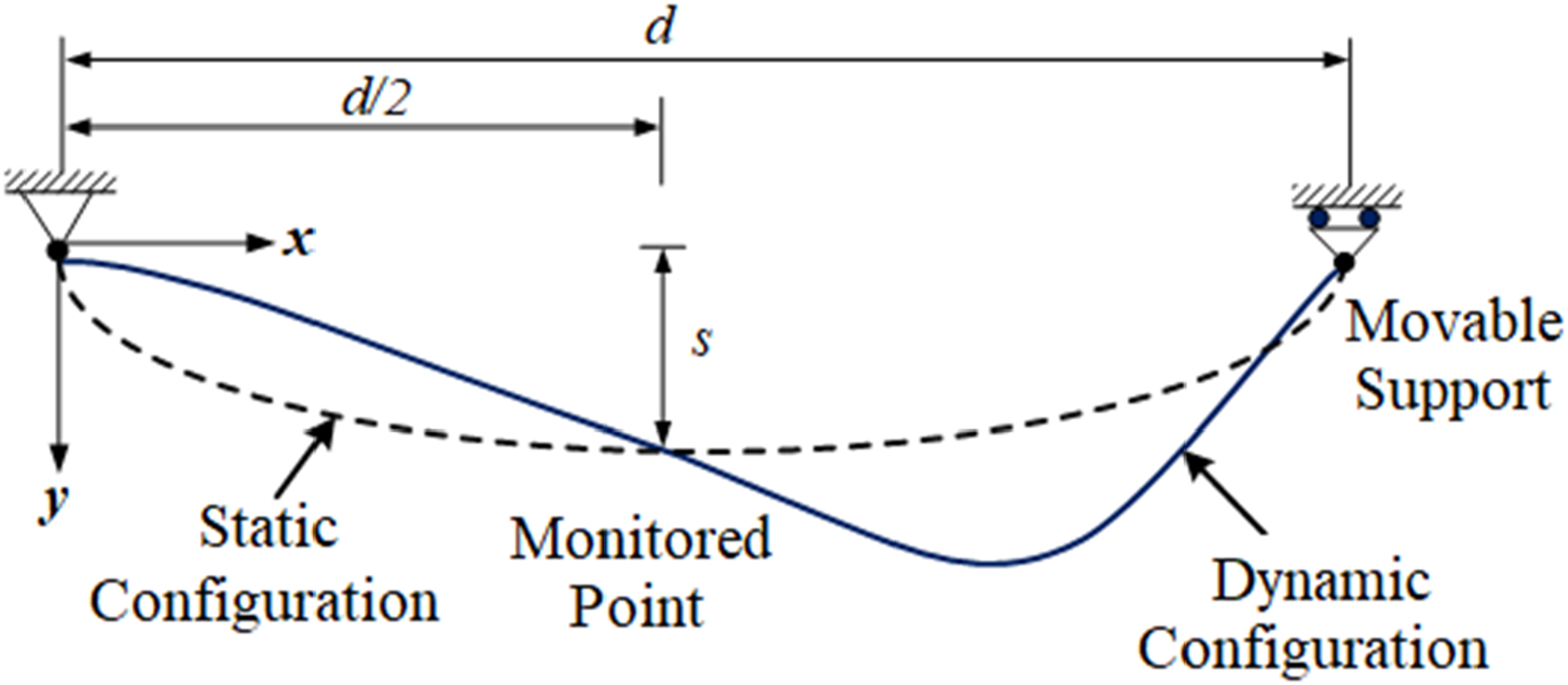
This part represents a dynamical cable system suspended between a fixed support and a movable support with a total span d, used to analyze the behavior of flexible cables under static and dynamic conditions. The static configuration, shown as a dashed line, represents the cable’s equilibrium shape under its weight, while the dynamic configuration, depicted as a solid curve, illustrates its deformation under external forces such as wind, vibrations, or moving loads. Displacements in the horizontal $u (x, t)$ and vertical $υ (x, t)$ directions are tracked over time and space, with a monitored point used to evaluate specific performance metrics. Also $s$ represents the initial sag of the cable at its lowest point, as shown in Figure 1. The movable support introduces additional dynamics, simulating boundary motion that impacts the cable’s response. This model is essential for predicting cable behavior, minimizing vibrations, and optimizing the stability and performance of structures like suspension bridges and cable-stayed systems.¹⁹

Figure 1.

The suspended cable system’s schematic (basic system).

Using the Hamilton variation principle, the nonlinear motion equation of the suspended cable is established while ignoring shear, torsional, and bending stiffness. The formula is provided by¹⁹

ρ_{m} \ddot{v} + 2 c \dot{v} - H v^{″} - \frac{E A}{d} (y^{″} + v^{″}) [\int_{0}^{d} (y^{'} v^{'} + 0.5 v^{' 2}) d x] = F_{e} (x, t),

(1)

where

ρ_{m}

represents the mass of the hung cable per unit length,

c

its coefficient of damping and

E

its elastic modulus. The symbols

A

refers to the hung cable’s cross-sectional area,

H

is its horizontal tension

(H = \frac{ρ_{m} g d^{2}}{8 s}, H \leq E A)

, and

g

expresses the acceleration brought on by gravity when applied to the right end of the moving support. The external excitation is represented by

F_{e} (x, t) = r (x) \cos Ω t

, where

Ω

denotes the frequency of the external excitation and

r (x)

represents the distribution function of this excitation.

The suspended cable’s sag-to-span ratio is thought to be rather low $(\frac{s}{d} < \frac{1}{8})$ , consequently, its form can be characterized as a parabola $y (x) = 4 s (\frac{x}{d}) [1 - (\frac{x}{d})] .$ presenting parameters without dimensions

x^{*} = x / d, y^{*} = y / d, v^{*} = v / d, β = E A / H, r^{*} = r d / H, t^{*} = t \sqrt{g / 8 s}, τ^{*} = τ \sqrt{g / 8 s}, Ω^{*} = Ω \sqrt{8 s / g}, c^{*} = (c / ρ_{m}) \sqrt{8 s / g} .

Once non-dimensionalization is done, (1) may be written as

\ddot{v} + 2 c \dot{v} - v^{″} - β (y^{″} + v^{″}) [\int_{0}^{d} (y^{'} v^{'} + 0.5 v^{' 2}) d x] = r (x) \cos Ω t .

(2)

Applying the Galerkin technique to discretize (2), it is assumed that the non-dimensional displacement function is

v (x, t) = q (t) ϕ (x),

(3)

where the mode function is denoted by

ϕ (x)

and the vibration’s function of displacement by

q (t)

.¹⁹ Through substituting (3) into (2), we obtain

\ddot{q} (t) + ω_{1}^{2} q (t) + μ_{1} \dot{q} (t) + \sum_{i, j = 1}^{\infty} Γ_{i j} q_{i} (t) q_{j} (t) + \sum_{i, j, k = 1}^{\infty} ρ_{i j k} q_{i} (t) q_{j} (t) q_{k} (t) = f \cos Ω t .

(4)

Here,

Γ_{i j} = - β \int_{0}^{1} [{ϕ_{j}}^{″} (x) \int_{0}^{1} {ϕ_{i}}^{'} (x) y^{'} d x] ϕ (x) d x - 0.5 β \int_{0}^{1} [y^{″} \int_{0}^{1} {ϕ_{j}}^{'} (x) {ϕ_{i}}^{'} (x) d x] ϕ (x) d x,

ρ_{i j k} = - 0.5 β \int_{0}^{1} [{ϕ_{j}}^{″} (x) \int_{0}^{1} {ϕ_{k}}^{'} (x) {ϕ_{i}}^{'} (x) d x] ϕ (x) d x, f = - \int_{0}^{1} r (x) ϕ (x) d x, μ_{1} = 2 \int_{0}^{1} c ϕ^{2} (x) d x .

This investigation primarily focuses on a single mode. To facilitate the description and manage nonlinear terms, we aim for a more thorough analysis of the nonlinear aspects response; a new time scale is presented $τ = ω_{1} t$ . It can be inserted into (4) to yield the following expression

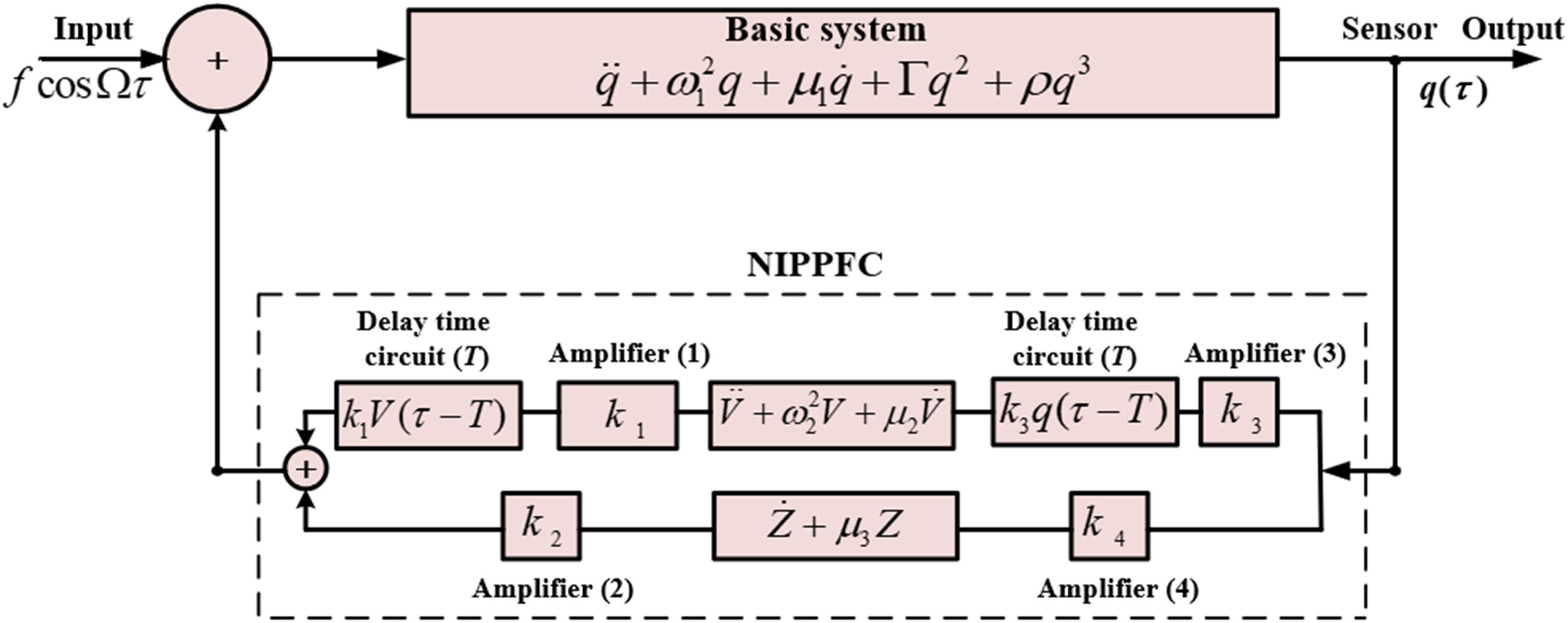
\ddot{q} (τ) + ω_{1}^{2} q (τ) + μ_{1} \dot{q} (τ) + Γ q^{2} (τ) + ρ q^{3} (τ) = f \cos Ω τ .

(5)

The non-dimensional (5) is modified by adding NIPPFC for lowering produced vibrations in the system, as shown in Figure 2. In light of these factors, the suspended cable system’s mathematical equation will be built as follows:

\ddot{q} (τ) + ω_{1}^{2} q (τ) + μ_{1} \dot{q} (τ) + Γ q^{2} (τ) + ρ q^{3} (τ) = f \cos Ω τ + k_{1} V (τ - T) + k_{2} Z (τ),

\ddot{V} (τ) + ω_{2}^{2} V (τ) + μ_{2} \dot{V} (τ) = k_{3} q (τ - T), \dot{Z} (τ) + μ_{3} Z (τ) = k_{4} q (τ) .

(6)

Here, the over-dot indicates a derivative with respect to

τ

μ_{1}, ω_{1}

are the basic system’s linear damping coefficient and resonant frequency, respectively. The notations

Γ

and

ρ

are the weak nonlinear stiffness coefficients,

Ω

and

f

show the excitation force’s frequency and amplitude, respectively. Whereas,

V (τ)

and

Z (τ)

indicate the NIPPFC’s second-order part variable and the integrating section variable, respectively. The controller’s internal frequency and damping factor are denoted by

ω_{2}

and

μ_{2}

, respectively. A positive scalar,

k_{1}

, represents the feedback gain in the second-order section, while the integrating section’s positive scalar feedback gain is denoted by

k_{2}

. The controller gains

k_{3}

and

k_{4}

point to such that

k_{3} > 0, k_{4} > 0 .

The notations

μ_{3}

and

T

represent the frequency of the loss integrator and time delay, respectively, as depicted in Figure 2.

Figure 2.

The NIPPFC of the suspended cable model.

The suggested strategy and resonance categorization

In this part, the MSA helps derive the approximate analytical solutions for equations (6). Thus, our analysis focuses on the system’s dynamic behavior in a small region around the stationary equilibrium point, incorporating the smallness of variables and parameters in accordance with

μ_{s} = ε {\tilde{μ}}_{s}, k_{j} = ε {\tilde{k}}_{j}, f = ε \tilde{f}, Γ = ε \tilde{Γ}, ρ = ε \tilde{ρ}; (s = 1, 2), (j = 1, 2, 3) .

(7)

where

0 < ε ≪ 1

is a tiny parameter.

Based on the MSA, the solutions $q, V,$ and $Z$ can be expressed as shown in the following illustration.²⁶

q = q_{0} (τ_{0}, τ_{1}) + ε q_{1} (τ_{0}, τ_{1}) + O (ε^{2}),

V = V_{0} (τ_{0}, τ_{1}) + ε V_{1} (τ_{0}, τ_{1}) + O (ε^{2}), Z = Z_{0} (τ_{0}, τ_{1}) + ε Z_{1} (τ_{0}, τ_{1}) + O (ε^{2}) .

(8)

Here,

τ_{n} = ε^{n} τ (n = 0, 1)

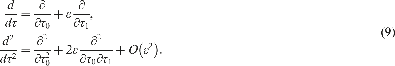
represent distinct time scales, where

τ_{0}

is fast and

τ_{1}

is slowly. It is essential to convert the derivatives with respect to

τ

into these scales. Therefore, to achieve this goal, the differential operators listed below can be utilized:

\frac{d}{d τ} = \frac{\partial}{\partial τ_{0}} + ε \frac{\partial}{\partial τ_{1}}, \frac{d^{2}}{d τ^{2}} = \frac{\partial^{2}}{\partial τ_{0}^{2}} + 2 ε \frac{\partial^{2}}{\partial τ_{0} \partial τ_{1}} + O (ε^{2}) .

(9)

Because of their tiny magnitude, these operators make it obvious that terms $O (ε^{2})$ and above are disregarded. The sets of partial DEs that correspond to the various powers of $ε$ are obtained by substituting (7)–(9) into equation (6).

(i) Order of $ε^{0}$

\frac{\partial^{2} q_{0}}{\partial τ_{0}^{2}} + ω_{1}^{2} q_{0} = 0,

(10)

\frac{\partial^{2} V_{0}}{\partial τ_{0}^{2}} + ω_{2}^{2} V_{0} = 0 .

(11)

\frac{\partial Z_{0}}{\partial τ_{0}} + μ_{3} Z_{0} = k_{4} q_{0} .

(12)

$(ii) Order of ε$

\frac{\partial^{2} q_{1}}{\partial τ_{0}^{2}} + ω_{1}^{2} q_{1} = \frac{1}{2} \tilde{f} e^{i Ω τ_{0}} - \tilde{Γ} q_{0}^{2} - \tilde{ρ} q_{0}^{3} + {\tilde{k}}_{1} V_{0 T} + {\tilde{k}}_{2} Z_{0} - {\tilde{μ}}_{1} \frac{\partial q_{0}}{\partial τ_{0}} - 2 \frac{\partial^{2} q_{0}}{\partial τ_{0} \partial τ_{1}},

(13)

\frac{\partial^{2} V_{1}}{\partial τ_{0}^{2}} + ω_{2}^{2} V_{1} = {\tilde{k}}_{3} q_{0 T} - {\tilde{μ}}_{2} \frac{\partial V_{0}}{\partial τ_{0}} - 2 \frac{\partial^{2} V_{0}}{\partial τ_{0} \partial τ_{1}},

(14)

\frac{\partial Z_{1}}{\partial τ_{0}} + μ_{3} Z_{1} = k_{4} q_{1} - \frac{\partial Z_{0}}{\partial τ_{1}} .

(15)

Because the previous equations (10)–(15) may be solved sequentially, the importance of the solutions provided by the main set of equations (10)–(12) is highlighted. Therefore, the following are the general solutions to (10) through (12).

q_{0} (τ) = B_{1} (τ_{1}) e^{i ω_{1} τ_{0}} + {\bar{B}}_{1} (τ_{1}) e^{- i ω_{1} τ_{0}},

(16)

V_{0} (τ) = B_{2} (τ_{1}) e^{i ω_{2} τ_{0}} + {\bar{B}}_{2} (τ_{1}) e^{- i ω_{2} τ_{0}},

(17)

Z_{0} (τ) = \frac{k_{4} B_{1} (τ_{1})}{μ_{3} + i ω_{1}} e^{i ω_{1} τ_{0}} + \frac{k_{4} {\bar{B}}_{1} (τ_{1})}{μ_{3} - i ω_{1}} e^{- i ω_{1} τ_{0}} .

(18)

Here,

B_{s} (s = 1, 2)

indicate obscured, intricate processes operating on time scales

τ_{1}

, whereas

{\bar{B}}_{i}

displays their complex conjugate.

Assume that

q (τ - T) = q_{T} = q_{0 T} (τ_{0}, τ_{1}) + ε q_{1 T} (τ_{0}, τ_{1}) + O (ε^{2}), V (τ - T) = V_{T} = V_{0 T} (τ_{0}, τ_{1}) + ε V_{1 T} (τ_{0}, τ_{1}) + O (ε^{2}),

(19)

q_{0 T} = B_{1 T} (τ_{1}) e^{i ω_{1} (τ_{0} - T)} + {\bar{B}}_{1 T} (τ_{1}) e^{- i ω_{1} (τ_{0} - T)}, V_{0 T} = B_{2 T} (τ_{1}) e^{i ω_{2} (τ_{0} - T)} + {\bar{B}}_{2 T} (τ_{1}) e^{- i ω_{2} (τ_{0} - T)},

(20)

Expanding $B_{s T} (τ_{1})$ in Taylor series, such that

B_{s T} (τ_{1}) = B_{s} (τ_{1}) - ε T {\dot{B}}_{s} (τ_{1}) + . . . . . .

(21)

Using simply the first term assumption and substituting (21) into (20), we get

q_{0 T} = B_{1} (τ_{1}) e^{i ω_{1} (τ_{0} - T)} + {\bar{B}}_{1} (τ_{1}) e^{- i ω_{1} (τ_{0} - T)}, V_{0 T} = B_{2} (τ_{1}) e^{i ω_{2} (τ_{0} - T)} + {\bar{B}}_{2} (τ_{1}) e^{- i ω_{2} (τ_{0} - T)},

(22)

It is possible to solve equations (13)–(15) by substituting the previous solutions’ responses to (16)–(18) and (22) by removing the secular terms. The following conditions are used to eliminate them.

- 2 i ω_{1} \frac{\partial B_{1}}{\partial τ_{1}} - i ω_{1} {\tilde{μ}}_{1} B_{1} - 3 \tilde{ρ} B_{1}^{2} {\bar{B}}_{1} + \frac{{\tilde{k}}_{2} k_{4}}{μ_{3} + i ω_{1}} B_{1} = 0,

(23)

- 2 i ω_{2} \frac{\partial B_{2}}{\partial τ_{1}} - i ω_{2} {\tilde{μ}}_{2} B_{2} = 0,

(24)

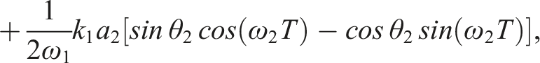
The next steps produce the second-order solutions, which are listed as follows:

q_{2} = \frac{\tilde{f}}{2 (ω_{1}^{2} - Ω^{2})} e^{i Ω τ_{0}} + \frac{\tilde{Γ} B_{1}^{2}}{3 ω_{1}^{2}} e^{2 i ω_{1} τ_{0}} + \frac{\tilde{ρ} B_{1}^{3}}{8 ω_{1}^{2}} e^{3 i ω_{1} τ_{0}} + \frac{{\tilde{k}}_{1} B_{2} e^{- i ω_{2} T}}{ω_{1}^{2} - ω_{2}^{2}} e^{i ω_{2} τ_{0}} - \frac{2 \tilde{Γ} B_{1} {\bar{B}}_{1}}{ω_{1}^{2}} + C C,

(25)

V_{2} = \frac{{\tilde{k}}_{3} B_{1} e^{- i ω_{1} T}}{ω_{2}^{2} - ω_{1}^{2}} e^{i ω_{1} τ_{0}} + C C,

(26)

Z_{2} = \frac{1}{24} k_{4} [\frac{12 \tilde{f} e^{i Ω τ_{0}}}{(ω_{1}^{2} - Ω^{2}) (μ_{3} + i Ω)} - \frac{12 {\tilde{k}}_{2} k_{4} B_{1} e^{i ω_{1} τ_{0}}}{ω_{1} {(ω_{1} - i μ_{3})}^{3}} - \frac{12 {\tilde{μ}}_{1} B_{1} e^{i ω_{1} τ_{0}}}{{(ω_{1} - i μ_{3})}^{2}} + \frac{8 \tilde{Γ} B_{1}^{2} e^{2 i ω_{1} τ_{0}}}{ω_{1}^{2} (μ_{3} + 2 i ω_{1})}

+ \frac{3 \tilde{ρ} B_{1}^{3} e^{3 i ω_{1} τ_{0}}}{ω_{1}^{2} (μ_{3} + 3 i ω_{1})} + \frac{24 {\tilde{k}}_{1} B_{2} e^{- i ω_{2} T} e^{i ω_{2} τ_{0}}}{(ω_{1}^{2} - ω_{2}^{2}) (μ_{3} + i ω_{2})} - \frac{48 \tilde{Γ} B_{1} {\bar{B}}_{1}}{ω_{1}^{2} μ_{3}} + \frac{36 \tilde{ρ} μ_{3} B_{1}^{2} {\bar{B}}_{1} e^{i ω_{1} τ_{0}}}{ω_{1} {(ω_{1} - i μ_{3})}^{3}} + \frac{36 \tilde{ρ} B_{1}^{2} {\bar{B}}_{1} e^{i ω_{1} τ_{0}}}{{(μ_{3} + i ω_{1})}^{3}}] + C C .

(27)

Here,

C C

demonstrates the conjugations of the preceding expressions.

We categorize resonance cases, handle one of them, and obtain the ME. If any of the denominators in the final two solution approaches disappear, these conditions could appear.³⁰ Consequently, the following possibilities arise.

• Primary external resonance is acquired at $Ω = ω_{1},$

• Internal resonance at $ω_{2} = ω_{1},$ and $ω_{1} = 0$ .

The system being studied will behave in a very complex way if any of the resonance requirements listed above are met. It’s important to keep in mind that even when waves are far from resonance, the solutions that are produced are still appropriate. Let’s now investigate the issue in more detail and look at a combination of the primary external and internal resonance that happened at exactly that duration, that is, $Ω \approx ω_{1}, ω_{2} \approx ω_{1}$ . The detuning factors $σ_{s} (s = 1, 2)$ that help achieve this goal can then be taken into consideration. Next, one can assume the detuning parameters $σ_{s} (s = 1, 2)$ that help accomplish this goal, which indicates the proximity of $Ω$ and $ω_{2}$ to $ω_{1}$ . As a result, one states:

Ω = ω_{1} + σ_{1}, ω_{2} = ω_{1} + σ_{2},

(28)

where

σ_{s} = ε {\tilde{σ}}_{s}

. Detuning parameters can also be thought of as a separation from the strict resonance and oscillations.³¹ Solvability requirements can be obtained by eliminating secular terms. As a consequence, the following formulas determine the probability that the requirements are fulfilled.

- 2 i ω_{1} \frac{\partial B_{1}}{\partial τ_{1}} - i ω_{1} {\tilde{μ}}_{1} B_{1} - 3 \tilde{ρ} B_{1}^{2} {\bar{B}}_{1} + \frac{{\tilde{k}}_{2} k_{4}}{μ_{3} + i ω_{1}} B_{1} + {\tilde{k}}_{1} B_{2} e^{- i ω_{2} T} e^{i {\tilde{σ}}_{2} τ_{1}} + \frac{1}{2} {\tilde{f}}_{1} e^{i {\tilde{σ}}_{1} τ_{1}} = 0, - 2 i ω_{2} \frac{\partial B_{2}}{\partial τ_{1}} - i ω_{2} {\tilde{μ}}_{2} B_{2} + {\tilde{k}}_{3} B_{1} e^{- i ω_{1} T} e^{- i {\tilde{σ}}_{2} τ_{1}} = 0 .

(29)

The obtained solvability condition (29), which depends on $τ_{1}$ , contains four nonlinear partial DEs with respect to $B_{s}$ .

Hence, we can utilize the subsequent polar form to present these functions:

B_{s} (τ_{1}) = \frac{{\tilde{a}}_{s} (τ_{1})}{2} e^{i α_{s} (τ_{1})}; a_{s} = ε {\tilde{a}}_{s} (s = 1, 2) .

(30)

As the functions $B_{s}$ are independent of the scale $τ_{0}$ , the first-order derivative operator can be expressed in a simplified form as follows

\frac{\partial B_{s}}{\partial τ_{0}} = 0, \frac{\partial B_{s}}{\partial τ} = ε \frac{\partial B_{s}}{\partial τ_{1}} .

(31)

Regarding (31), the modified phases below can transform the solvability criteria of partial DEs (29) into ordinary differential equations

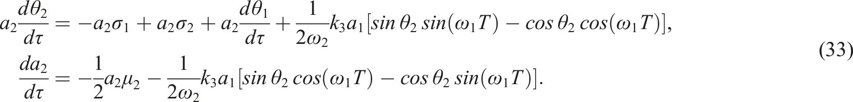
θ_{1} (τ_{1}) = τ_{1} {\tilde{σ}}_{1} - α_{1} (τ_{1}), θ_{2} (τ_{1}) = τ_{1} {\tilde{σ}}_{2} - α_{1} (τ_{1}) + α_{2} (τ_{1}) .

(32)

By dividing the real and imaginary components and inserting (30)–(32) into (29), the system below can be produced depending on the preceding

a_{1} \frac{d θ_{1}}{d τ} = a_{1} σ_{1} - \frac{3}{8} ρ a_{1}^{3} + \frac{μ_{3} k_{2} k_{4}}{2 (μ_{3}^{2} + ω_{1}^{2})} a_{1} + \frac{1}{2 ω_{1}} f \cos θ_{1}

+ \frac{1}{2 ω_{1}} k_{1} a_{2} [\sin θ_{2} \sin (ω_{2} T) + \cos θ_{2} \cos (ω_{2} T)],

\frac{d a_{1}}{d τ} = - \frac{1}{2} a_{1} μ_{1} - \frac{k_{2} k_{4}}{2 (μ_{3}^{2} + ω_{1}^{2})} a_{1} + \frac{1}{2 ω_{1}} f \sin θ_{1}

+ \frac{1}{2 ω_{1}} k_{1} a_{2} [\sin θ_{2} \cos (ω_{2} T) - \cos θ_{2} \sin (ω_{2} T)],

a_{2} \frac{d θ_{2}}{d τ} = - a_{2} σ_{1} + a_{2} σ_{2} + a_{2} \frac{d θ_{1}}{d τ} + \frac{1}{2 ω_{2}} k_{3} a_{1} [\sin θ_{2} \sin (ω_{1} T) - \cos θ_{2} \cos (ω_{1} T)], \frac{d a_{2}}{d τ} = - \frac{1}{2} a_{2} μ_{2} - \frac{1}{2 ω_{2}} k_{3} a_{1} [\sin θ_{2} \cos (ω_{1} T) - \cos θ_{2} \sin (ω_{1} T)] .

(33)

Steady-state strategies and analyzing stability

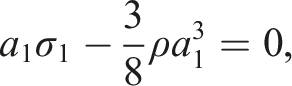
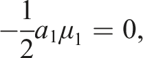
In this section, we concentrate on the solutions corresponding to the system’s steady-state condition. In this scenario, the solutions would be displayed at the final stage of the temporary procedures. We consider $\frac{d a_{s}}{d τ} = \frac{d θ_{s}}{d τ}$ to have a value of zero in this scenario, where $(s = 1, 2)$ .²⁷ Accordingly, equation (33) lead to generate the following algebraic equations

\frac{μ_{3} k_{2} k_{4}}{2 (μ_{3}^{2} + ω_{1}^{2})} a_{1} + \frac{1}{2 ω_{1}} f \cos θ_{1} + \frac{1}{2 ω_{1}} k_{1} a_{2} [\sin θ_{2} \sin (ω_{2} T) + \cos θ_{2} \cos (ω_{2} T)]

a_{1} σ_{1} - \frac{3}{8} ρ a_{1}^{3} = 0,

- \frac{k_{2} k_{4}}{2 (μ_{3}^{2} + ω_{1}^{2})} a_{1} + \frac{1}{2 ω_{1}} f \sin θ_{1} + \frac{1}{2 ω_{1}} k_{1} a_{2} [\sin θ_{2} \cos (ω_{2} T) - \cos θ_{2} \sin (ω_{2} T)]

- \frac{1}{2} a_{1} μ_{1} = 0,

- a_{2} σ_{1} + a_{2} σ_{2} + \frac{1}{2 ω_{2}} k_{3} a_{1} [\sin θ_{2} \sin (ω_{1} T) - \cos θ_{2} \cos (ω_{1} T)] = 0, - \frac{1}{2} a_{2} μ_{2} - \frac{1}{2 ω_{2}} k_{3} a_{1} [\sin θ_{2} \cos (ω_{1} T) - \cos θ_{2} \sin (ω_{1} T)] = 0 .

(34)

Based on the analysis of the previous system (34), with the removal of the modified phases $θ_{1}$ and $θ_{2}$ , the following frequency response equations are obtained.

f_{1}^{2} + 2 a_{2} k_{1} f_{1} (\cos ω_{2} T - \sin ω_{2} T) + k_{1}^{2} a_{2}^{2}

= ω_{1}^{2} \{{(\frac{3}{4} ρ a_{1}^{3} - 2 σ_{1} a_{1} - \frac{μ_{3} k_{2} k_{4}}{(μ_{3}^{2} + ω_{1}^{2})} a_{1})}^{2} + {(μ_{1} a_{1} + \frac{k_{2} k_{4}}{(μ_{3}^{2} + ω_{1}^{2})} a_{1})}^{2}\}, a_{1}^{2} = \frac{ω_{2}^{2}}{k_{3}^{2}} \{{(μ_{2} a_{2})}^{2} + 4 {(σ_{1} a_{2} - σ_{2} a_{2})}^{2}\} .

(35)

The following system is obtained by linearizing (33) using the Lyapunov first (indirect) technique, which is used to examine the stability characteristic of these solutions²⁸

[\begin{array}{l} {\dot{a}}_{1} \\ {\dot{θ}}_{1} \\ {\dot{a}}_{2} \\ {\dot{θ}}_{2} \end{array}] = [J] [\begin{array}{l} a_{1} \\ θ_{1} \\ a_{2} \\ θ_{2} \end{array}] = [\begin{array}{l} J_{11} J_{12} J_{13} J_{14} \\ J_{21} J_{22} J_{23} J_{24} \\ J_{31} J_{32} J_{33} J_{34} \\ J_{41} J_{42} J_{43} J_{44} \end{array}] [\begin{array}{l} a_{1} \\ θ_{1} \\ a_{2} \\ θ_{2} \end{array}],

(36)

where

J_{n m}; (n, m = 1 : 4)

are expressed in the Appendix.

Thus, the stability of the steady-state solution relies on our ability to evaluate and resolve the characteristic equation. The characteristic equation of the Jacobian matrix is represented as follows:³¹

| \begin{array}{l} J_{11} - λ J_{12} J_{13} J_{14} \\ J_{21} J_{22} - λ J_{23} J_{24} \\ J_{31} J_{32} J_{33} - λ J_{34} \\ J_{41} J_{42} J_{43} J_{44} - λ \end{array} | = 0,

(37)

λ^{4} + Γ_{1} λ^{3} + Γ_{2} λ^{2} + Γ_{3} λ + Γ_{4} = 0 .

(38)

Here,

Γ_{1}

represents a negative of the sum of the diagonal elements of

[J]

Γ_{2}

refers to the sum of the principal minors (determinants of 2 × 2 sub-matrices on the diagonal),

Γ_{3}

denotes the negative of the sum of determinants of 3 × 3 sub-matrices and

Γ_{4}

is the determinant of

[J]

. These coefficients have the forms

Γ_{1} = - (J_{11} + J_{22} + J_{33} + J_{44}),

Γ_{2} = J_{11} J_{22} + J_{11} J_{33} + J_{11} J_{44} + J_{22} J_{33} + J_{22} J_{44} + J_{33} J_{44}

- (J_{12} J_{21} + J_{13} J_{31} + J_{14} J_{41} + J_{23} J_{32} + J_{24} J_{42} + J_{34} J_{43}),

Γ_{3} = - (J_{11} \det (M_{11}) + J_{22} \det (M_{22}) + J_{33} \det (M_{33}) + J_{44} \det (M_{44})), Γ_{4} = \det (J) .

(39)

Here,

M_{11} = [\begin{array}{l} J_{22} J_{23} J_{24} \\ J_{32} J_{33} J_{34} \\ J_{42} J_{43} J_{44} \end{array}], M_{22} = [\begin{array}{l} J_{11} J_{13} J_{14} \\ J_{31} J_{33} J_{34} \\ J_{41} J_{43} J_{44} \end{array}], M_{33} = [\begin{array}{l} J_{11} J_{12} J_{14} \\ J_{21} J_{22} J_{24} \\ J_{41} J_{42} J_{44} \end{array}], M_{44} = [\begin{array}{l} J_{11} J_{12} J_{13} \\ J_{21} J_{22} J_{23} \\ J_{31} J_{32} J_{33} \end{array}] .

The solution’s state is asymptotically stable if and only if all real parts of the roots of (38) are negative, according to the Routh–Hurwitz condition.³³ This scenario arises if the coefficients satisfy

Γ_{1} > 0, Γ_{3} (Γ_{1} Γ_{2} - Γ_{3}) - Γ_{4} {Γ_{1}}^{2} > 0, Γ_{1} Γ_{2} - Γ_{3} > 0, Γ_{4} > 0,

(40)

which are numerically analyzed.

Results and discussion

This section examines both the controlled and uncontrolled scenarios, including the resonance condition, to demonstrate the system’s performance in terms of amplitude and phase. We examine the effects of particular factors on system amplitude and compare various control schemes. We also investigate the connection between the detuning parameters $σ_{s} (s = 1, 2)$ and the system amplitude. As well as compute Poincaré maps and perform bifurcation analysis to determine the stability and chaotic behavior of the system. Additionally, the system (33) of the aforementioned modulation can be numerically solved using the RK-4 to show how the functions $q, V, Z,$ and their associated phase planes behave at resonance with and without control. Consequently, the following initial conditions and data are considered

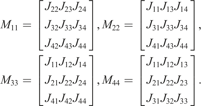
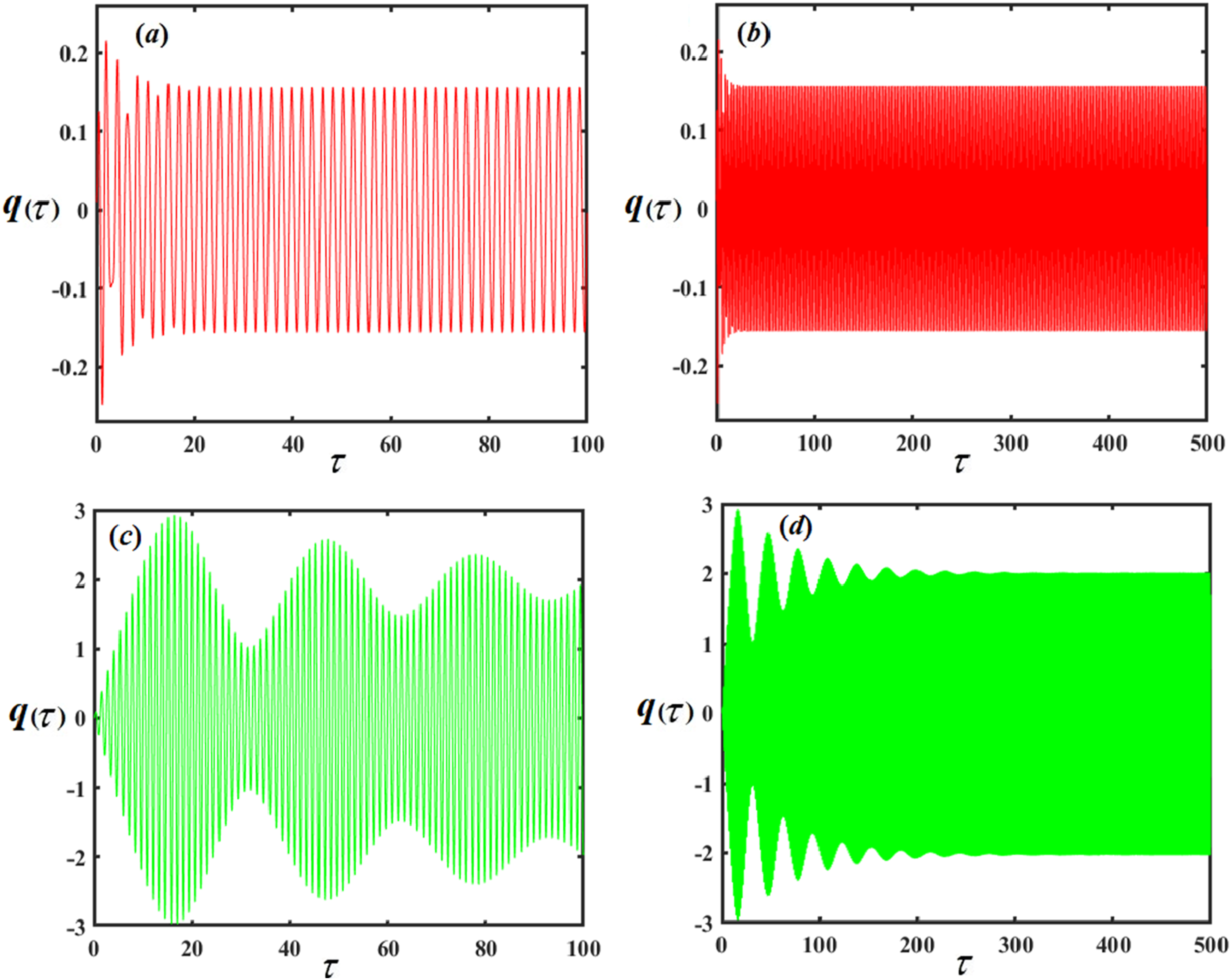
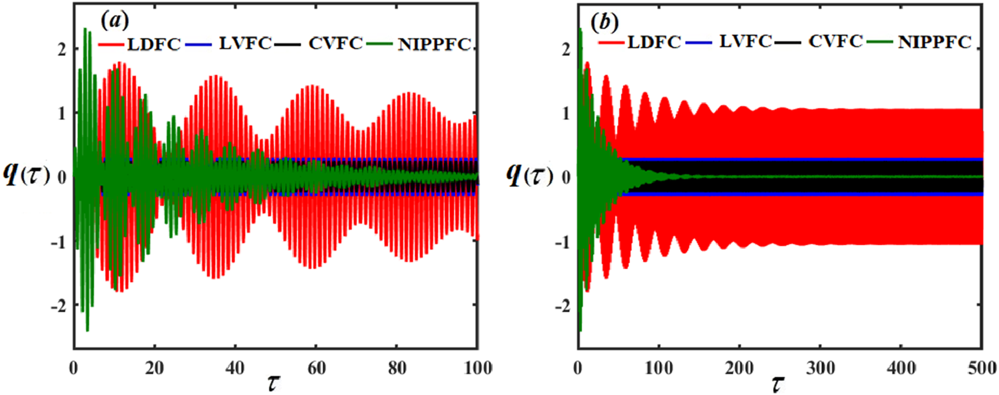
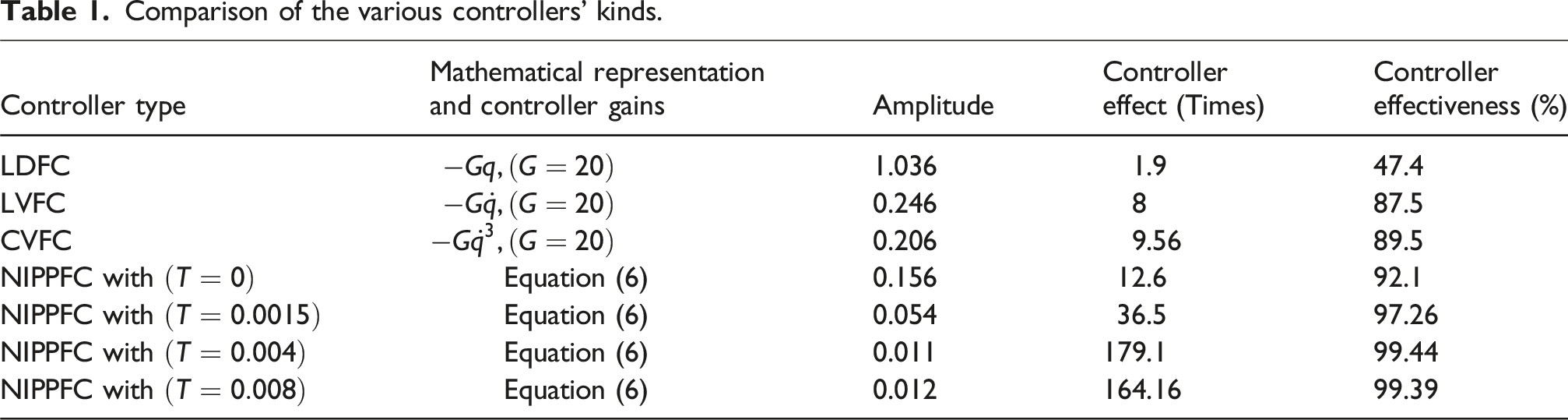
μ_{1} = 0.03, μ_{2} = 0.02, μ_{3} = 0.2, ω_{1} = 5, ω_{2} = 5, Ω = 5, f = 2.5, k_{1} = 20, k_{2} = 2, k_{3} = 1, k_{4} = 1.5, Γ = 0.2, ρ = 0.4, T = 0.004, a_{1} (0) = 0, a_{2} (0) = 0, θ_{1} (0) = 0.5, θ_{2} (0) = 0 .

For short and long time scales, respectively, Figure 3 displays the time history of the function $q$ in the basic case (without resonance and without control) as red and at resonance without control as light green. We observe that the amplitudes of waves during the basic case and the resonance case without control are, respectively, 0.156 and 1.97, indicating a threat to the system. The system must remain operational by controlling and minimizing these harmful vibrations. On the other hand, Figure 4 displays the time history of the same function $q$ at resonance with different kinds of controllers for both short and long time scales, in which the red color refers to LDFC $(k_{1} = 20)$ with an amplitude of the function $q$ equal to 1.036; therefore, the amplitude of $q$ is reduced by 47.4%, blue color point to LVFC $(k_{1} = 20)$ with an amplitude of 0.246, so the amplitude of $q$ is reduced by 87.5%; black color refers to CVFC $(k_{1} = 20)$ with the amplitude of 0.206; therefore, the amplitude of $q$ is reduced by 89.5%, the green represents NIPPFC with $(T = 0.004)$ and gains $(k_{1} = 20, k_{2} = 2, k_{3} = 1, k_{4} = 1.5)$ with the amplitude of 0.011, so the amplitude of $q$ is reduced by 99.44%; for this data, the NIPPFC is the best type. Figure 5 displays the time history of the same function $q$ at resonance with the nonlinear integral positive position feedback controller without time delay (NIPPF) and NIPPFC with $(T = 0.004)$ for both short and long time scales, we observe that the NIPPFC with $(T = 0.004)$ is the best. Figure 6 shows the time variation of the function $q$ at resonance with NIPPFC with multi-time delay $(T = 0.0015, 0.004, 0.008)$ for both short and long time scales, we observe that the NIPPFC with $(T = 0.004)$ is the best. The prior results are summarized in Table 1.

Figure 3.

Time response solution $q (τ)$ at various scales of $τ$ (a, b) at the basic case, (c, d) at resonance without control.

Figure 4.

The time response solution $q (τ)$ at various scales of $τ$ in resonance case with various types of controllers.

Figure 5.

Comparison between the time history of $q (τ)$ at various scales of $τ$ at resonance with the NIPPF and NIPPFC with $(T = 0.004)$ .

Figure 6.

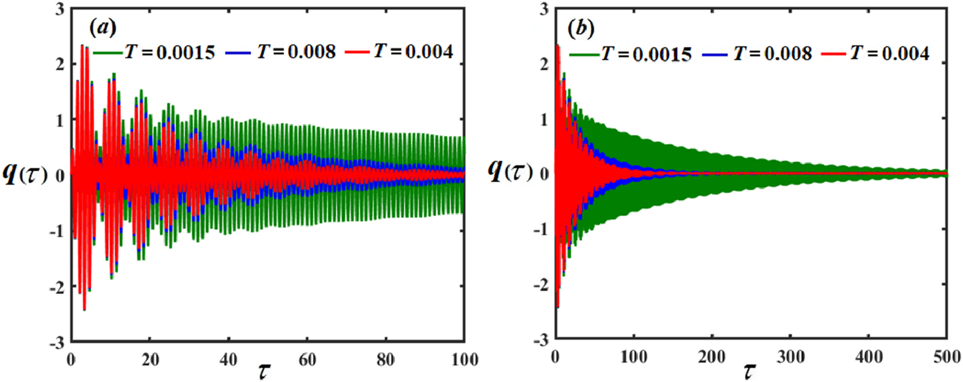
Comparison between the time history of $q (τ)$ at resonance with NIPPFC with different values of time delay at various scales of $τ$ .

Table 1.

Comparison of the various controllers’ kinds.

Controller type	Mathematical representation and controller gains	Amplitude	Controller effect (Times)	Controller effectiveness (%)
LDFC	$- G q, (G = 20)$	1.036	1.9	47.4
LVFC	$- G \dot{q}, (G = 20)$	0.246	8	87.5
CVFC	$- G {\dot{q}}^{3}, (G = 20)$	0.206	9.56	89.5
NIPPFC with $(T = 0)$	Equation (6)	0.156	12.6	92.1
NIPPFC with $(T = 0.0015)$	Equation (6)	0.054	36.5	97.26
NIPPFC with $(T = 0.004)$	Equation (6)	0.011	179.1	99.44
NIPPFC with $(T = 0.008)$	Equation (6)	0.012	164.16	99.39

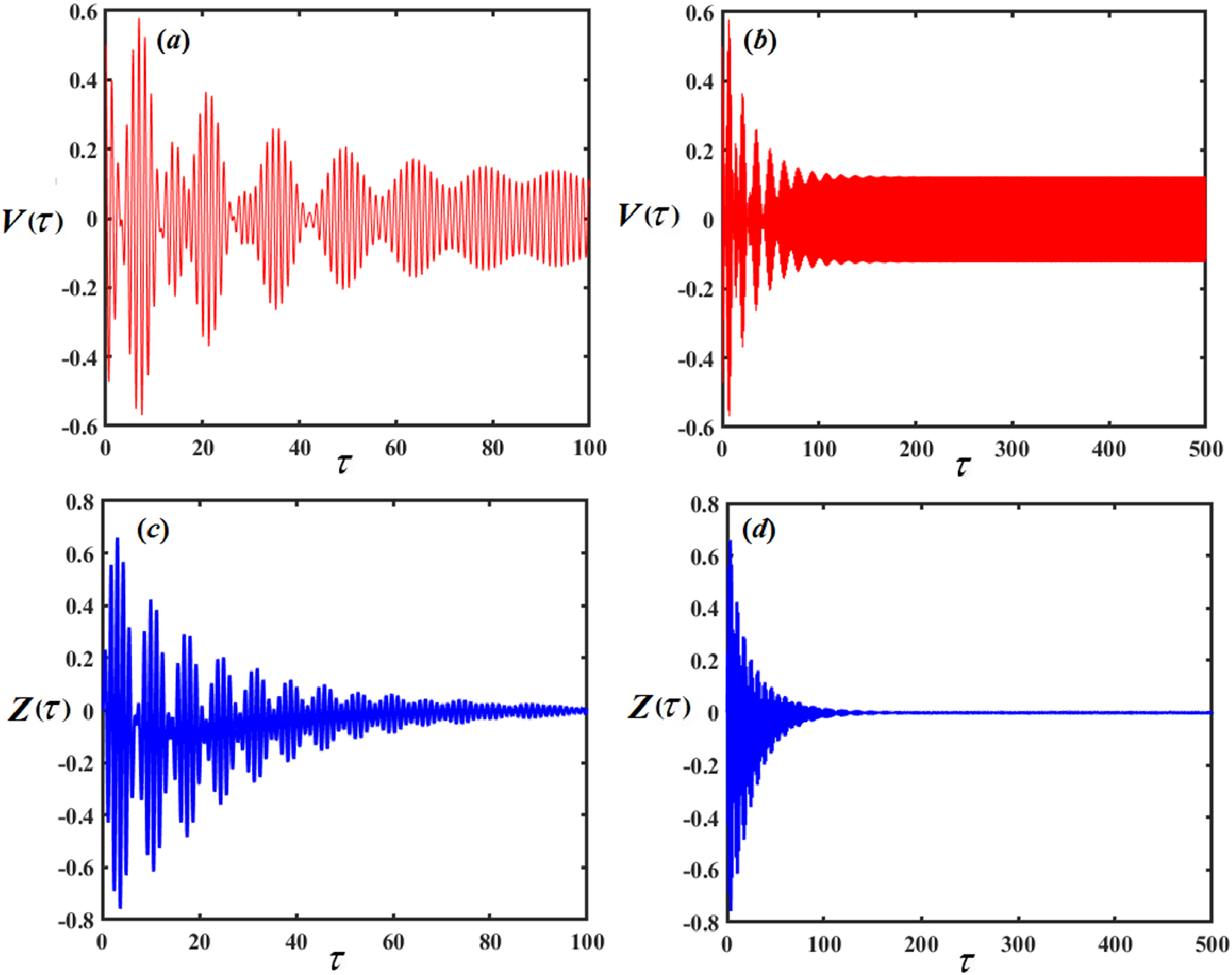
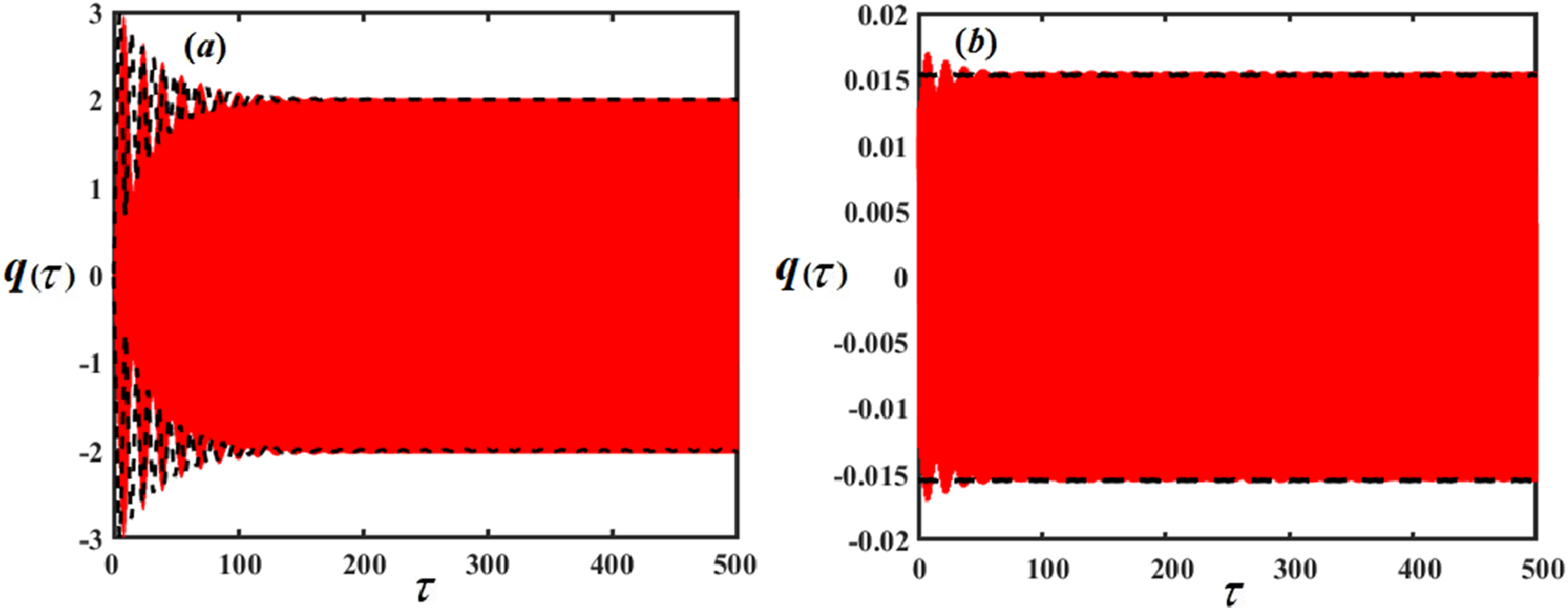
Figure 7 shows the time history of the functions $V$ and $Z$ at resonance with NIPPFC with $(T = 0.004)$ for both short and long-term scales. The AS driven by MSA and the NS utilizing RK-4 at the resonance case without control are contrasted by the curves in Figure 8(a). However, Figure 8(b) shows the comparison of the AS and the NS for the resonance case with NIPPFC with $(T = 0.004) .$ There is a great deal of agreement between the numerical and analytical solutions.

Figure 7.

The time history of the controllers $V$ and $Z$ at resonance with NIPPFC with $(T = 0.004)$ at various scales of $τ$ .

Figure 8.

The variation between AS, shown by the black line, and NS, shown by the red line, in resonance cases $(Ω = ω_{1}, ω_{2} = ω_{1})$ (a) without control, (b) with NIPPFC with $(T = 0.004)$ .

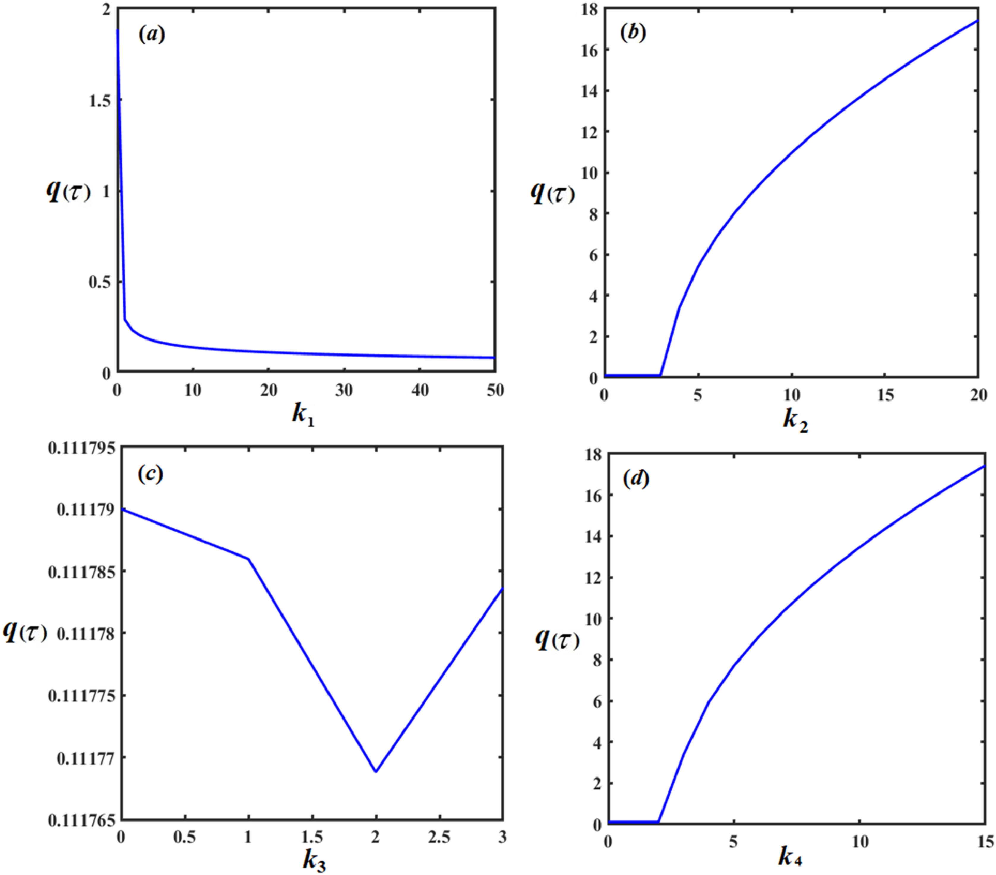
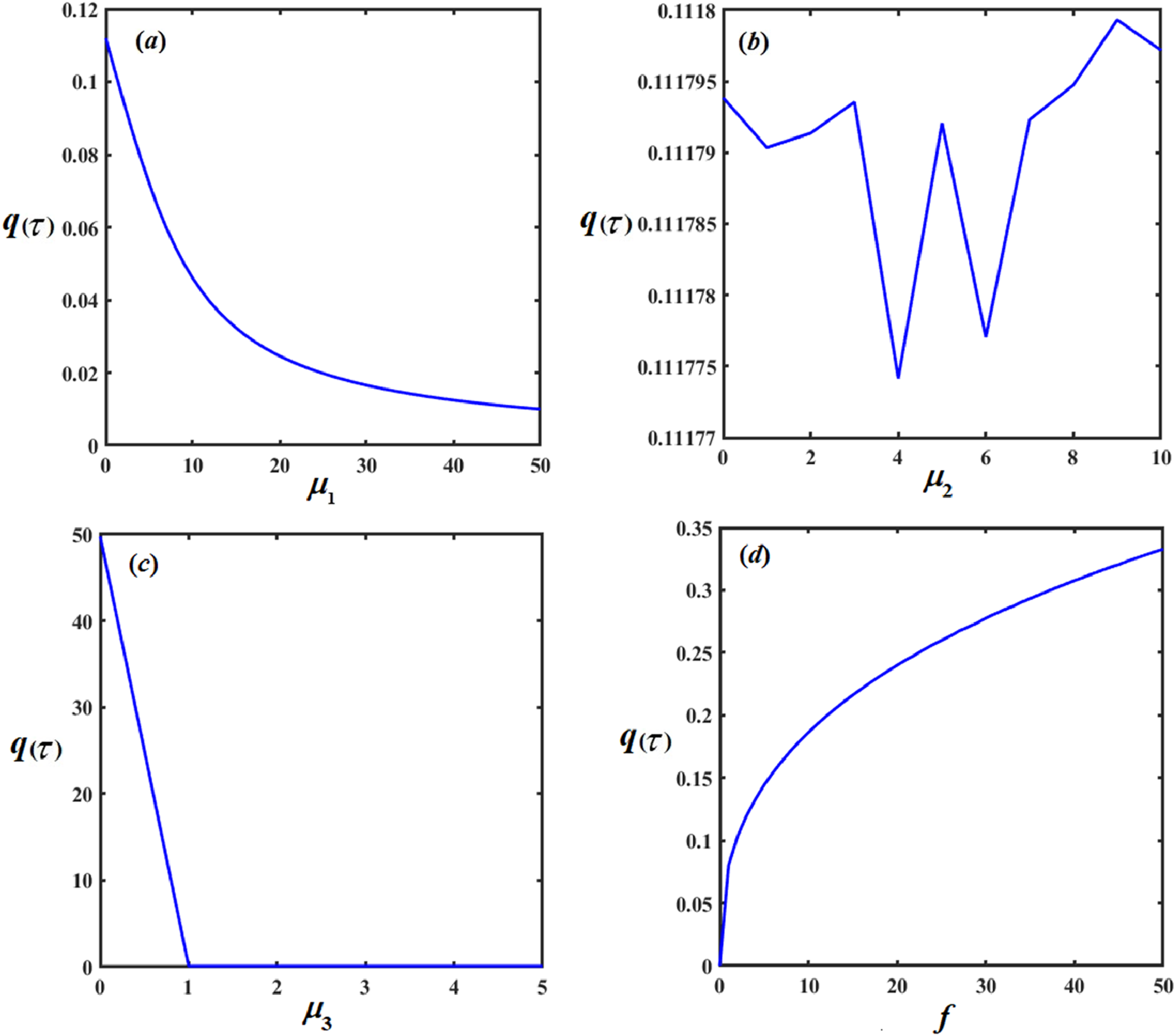
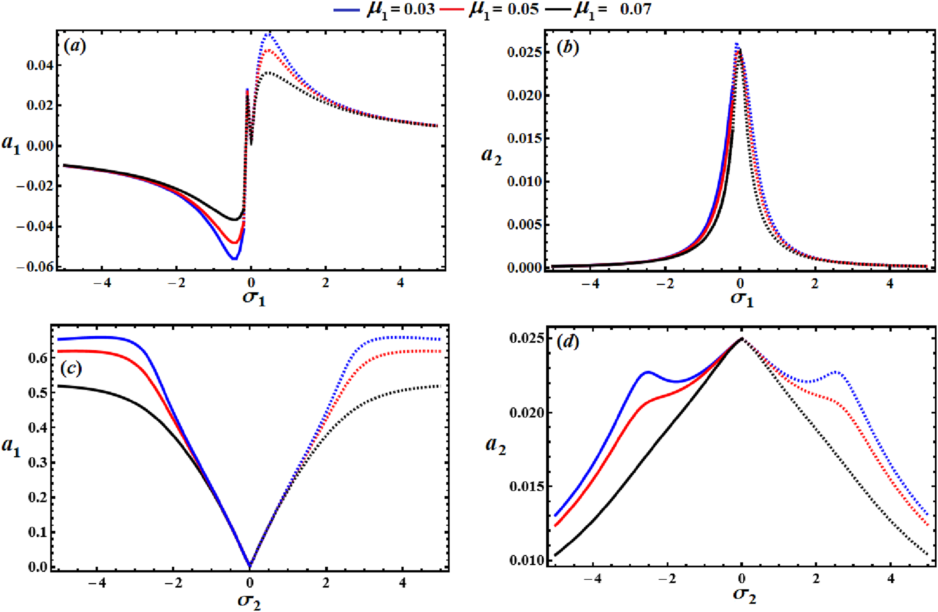
We will show how the amplitude of $q (τ)$ changes with the system parameters, $k_{1}, k_{2}, k_{3}, k_{4}, μ_{1}, μ_{2}, μ_{3},$ and $f$ are changed. It is noticed that when $k_{1}, k_{3}, μ_{1}$ and $μ_{3}$ values grow, the amplitude’s $q (τ)$ value falls. Although $k_{2}$ and $k_{4}$ have no influence on $q (τ)$ at first, they eventually cause it to rise, but the effect of $μ_{2}$ on $q (τ)$ is oscillating. On the other hand, when $f$ increases, $(τ)$ ’s amplitude also increases, as shown in Figures 9 and 10.

Figure 9.

System parameter effects $k_{1}, k_{2}, k_{3},$ and $k_{4}$ on the amplitude of the system $q (τ)$ .

Figure 10.

System parameter effects $μ_{1}, μ_{2}, μ_{3},$ and $f$ on the amplitude of the system $q (τ)$ .

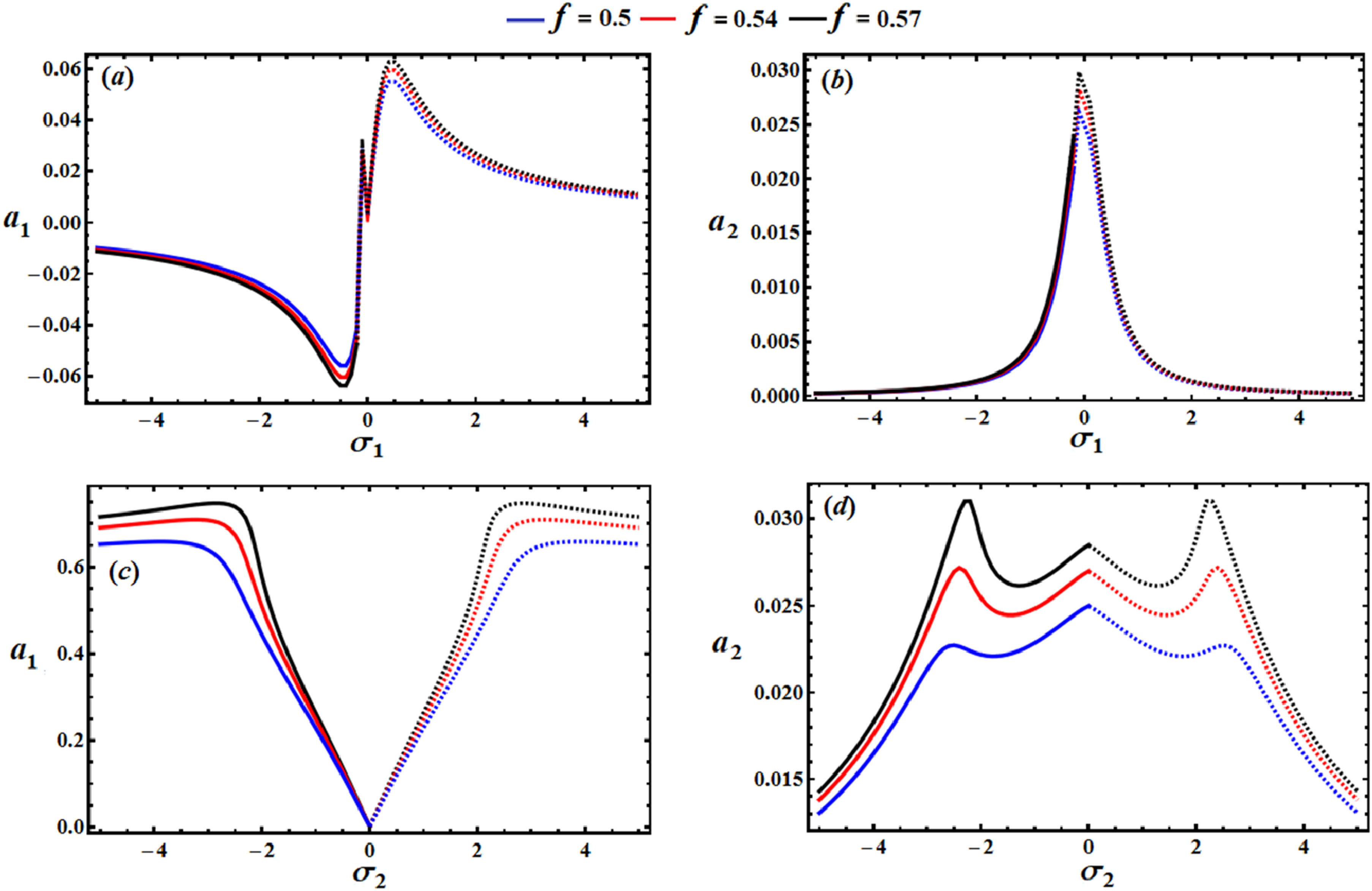
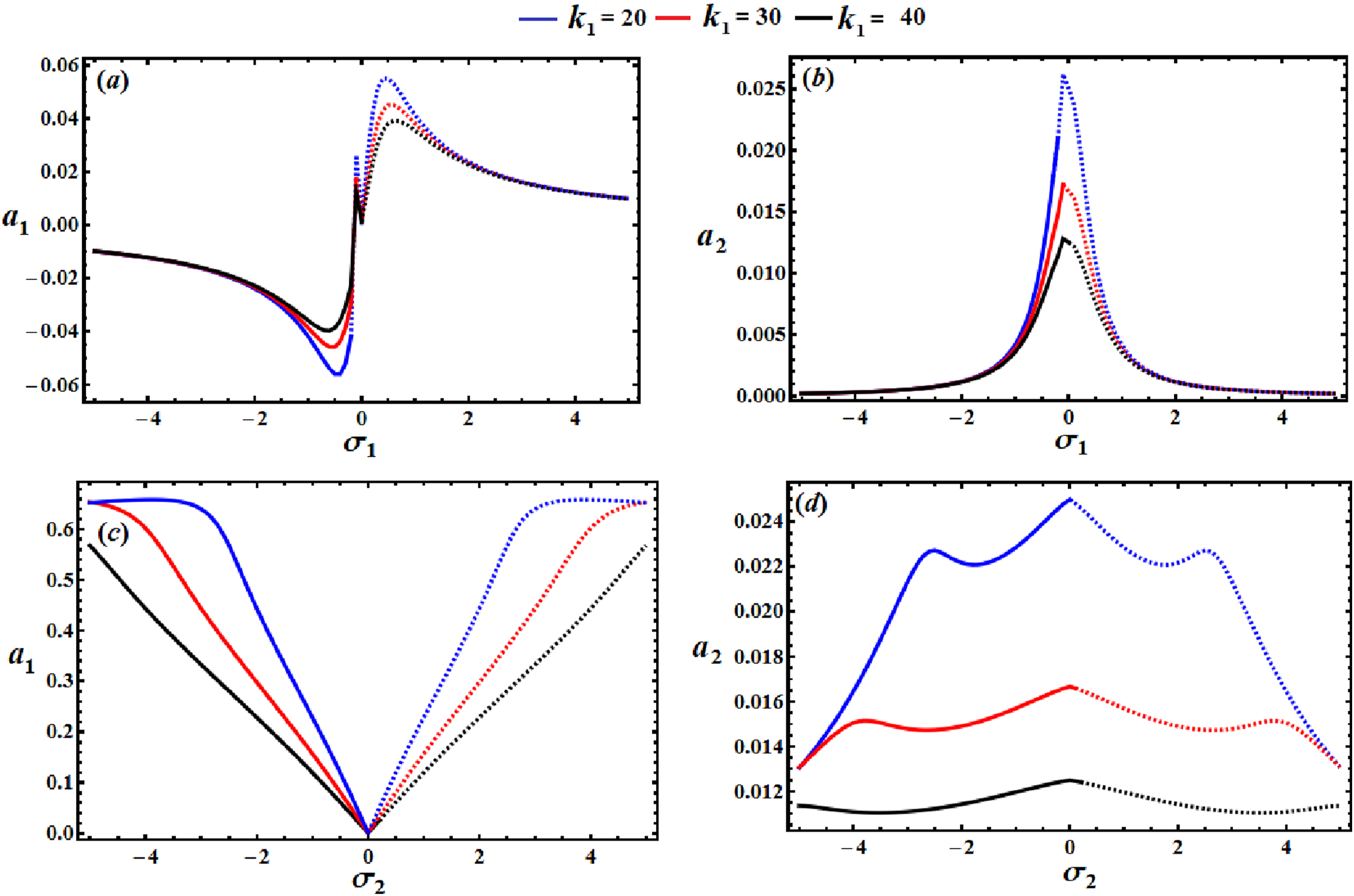
The resonant curves of response that are obtained from the NS of (24), illustrated in Figures 11–13 will indicate the stability zones of fixed points. Keep in mind that dashed lines denote unstable fixed points, whereas solid lines signify stable ones. Certain stability criterion factors, including controller gain $k_{1}$ , damping coefficient $μ_{1}$ , and excitation amplitude of force $f$ , were demonstrated to affect stability analysis significantly. As the values provided for the system parameters vary, Figures 11–13 display the system amplitude $q (τ)$ versus the detuning parameter $σ_{i}, (i = 1, 2)$ . As the values of $k_{1}$ and $μ_{1}$ grow, we see the amplitude decrease, as shown in Figures 12–13 but as the value of $f$ rises, the amplitude increases, as shown in Figure 11. The ranges that represent the zones of stability and instability in Figure 11(a) and (b) are $σ_{1} \leq - 0.2$ and $- 0.2 < σ_{1}$ , respectively, but the stability and instability regions in Figure 11(c) and (d) are $σ_{2} \leq 0$ and $0 < σ_{2}$ , respectively. The ranges in Figure 12(a) and (b) that correspond to the domains of stability and instability are $σ_{1} \leq - 0.2$ and $- 0.2 < σ_{1}$ for the blue curve and $σ_{1} \leq - 0.1$ and $- 0.1 < σ_{1}$ for the red curve, as well as $σ_{1} \leq 0$ and $0 < σ_{1}$ for the black curve. However, the stability and instability areas in Figure 12(c) and (d) are $σ_{1} \leq 0$ and $0 < σ_{1}$ for the blue color and $σ_{1} \leq 0.1$ and $0.1 < σ_{1}$ for the red curve, as well as $σ_{1} \leq 0.2$ and $0.2 < σ_{1}$ for the black curve. The domains that show stability and instability areas in Figure 13(a) and (b) are $σ_{1} \leq - 0.2$ and $- 0.2 < σ_{1}$ , respectively, but the stability and instability zones in Figure 13(c) and (d) are $σ_{2} \leq 0$ and $0 < σ_{2}$ , respectively.

Figure 11.

Amplitudes’ resonance curves $a_{s} (s = 1, 2)$ : (a), (b) versus $σ_{1}; σ_{2} = 0$ , (c), (d) versus $σ_{2}; σ_{1} = 0$ with NIPPFC with $(T = 0.004)$ .

Figure 12.

Resonance curves for amplitudes $a_{s}$ : (a), (b) versus $σ_{1}; σ_{2} = 0$ , (c), (d) versus $σ_{2}; σ_{1} = 0$ with NIPPFC with $(T = 0.004)$ .

Figure 13.

Resonance curves for amplitudes $a_{s}$ : (a), (b) versus $σ_{1}; σ_{2} = 0$ , (c), (d) vs $σ_{2}; σ_{1} = 0$ with NIPPFC with $(T = 0.004)$ .

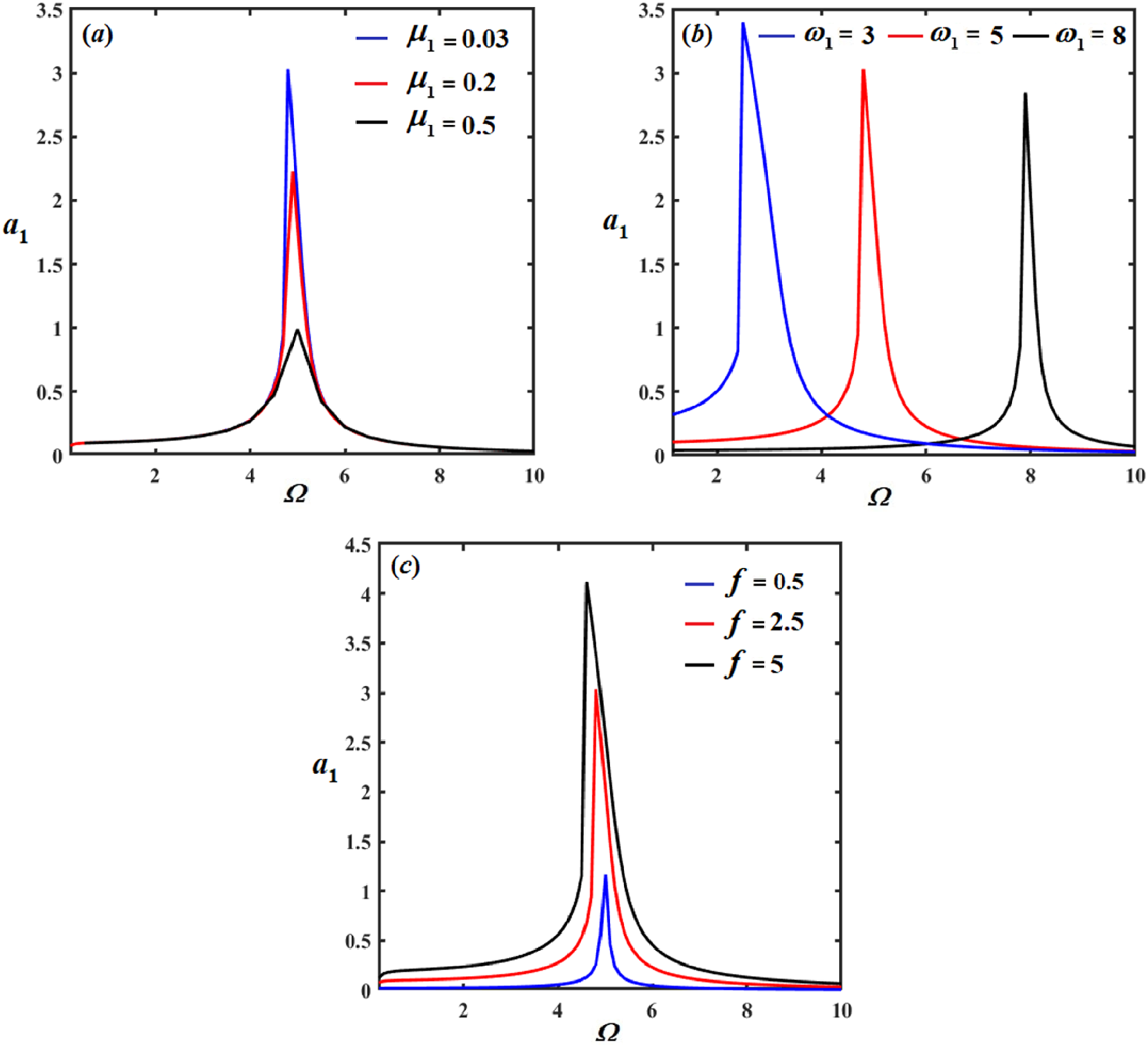
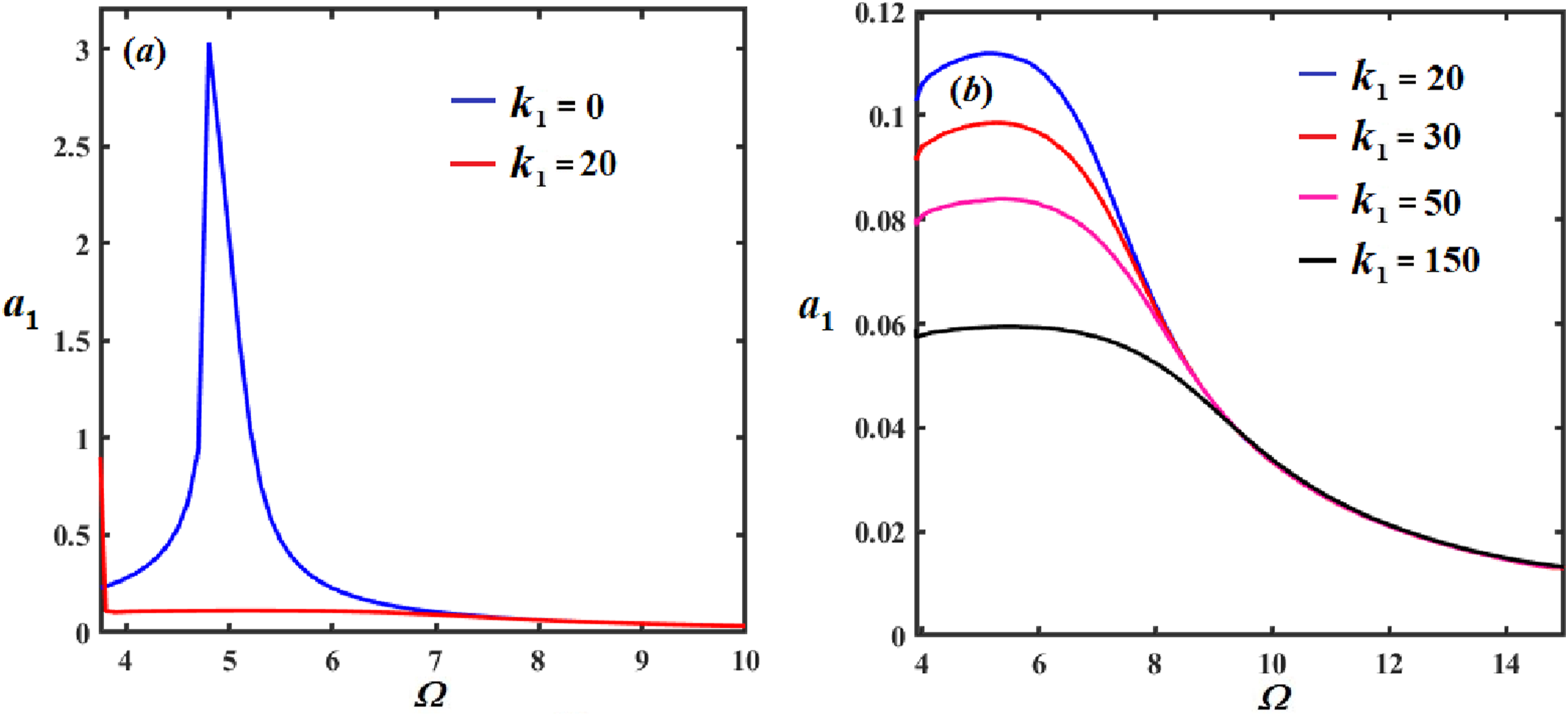
A dynamical system’s frequency response curve illustrates how the response of the system’s amplitude varies with the frequency of the excitation range. The amplitude-frequency behavior of the system without control $(k_{1} = k_{2} = k_{3} = k_{4} = 0)$ under various $μ_{1}$ , $ω_{1}$ , and $f$ values is shown in Figure 14. The system amplitude $a_{1}$ is decreased with increasing the coefficient of damping $μ_{1}$ , as explored in Figure 14(a) while Figure 14(b) shows the greatest amplitude at $Ω = ω_{1},$ As shown in Figure 14(c), the amplitude increases with the increase of the amplitude $f$ . Figure 15(a) presents the amplitude response without control $(k_{1} = k_{2} = k_{3} = k_{4} = 0)$ with a blue line and with NIPPFC $(k_{1} = 20, k_{2} = 2, k_{3} = 1, k_{4} = 1.5)$ with $(T = 0.004)$ with a red line. As the controller gain is increased $(k_{1} = 20, k_{1} = 30, k_{1} = 50, k_{1} = 150)$ , the system’s amplitude decreases, as explored in Figure 15(b).

Figure 14.

Amplitude–frequency curve $a_{1}$ without control $(k_{1} = k_{2} = k_{3} = k_{4} = 0)$ .

Figure 15.

(a) Amplitude–frequency curve $a_{1}$ without control $(k_{1} = k_{2} = k_{3} = k_{4} = 0)$ and with NIPPFC $(k_{1} = 20, k_{2} = 2, k_{3} = 1, k_{4} = 1.5)$ with $(T = 0.004)$ (b) Amplitude–frequency curve $a_{1}$ at different values of controller gain $(k_{1} = 20, k_{1} = 30, k_{1} = 50, k_{1} = 150)$ .

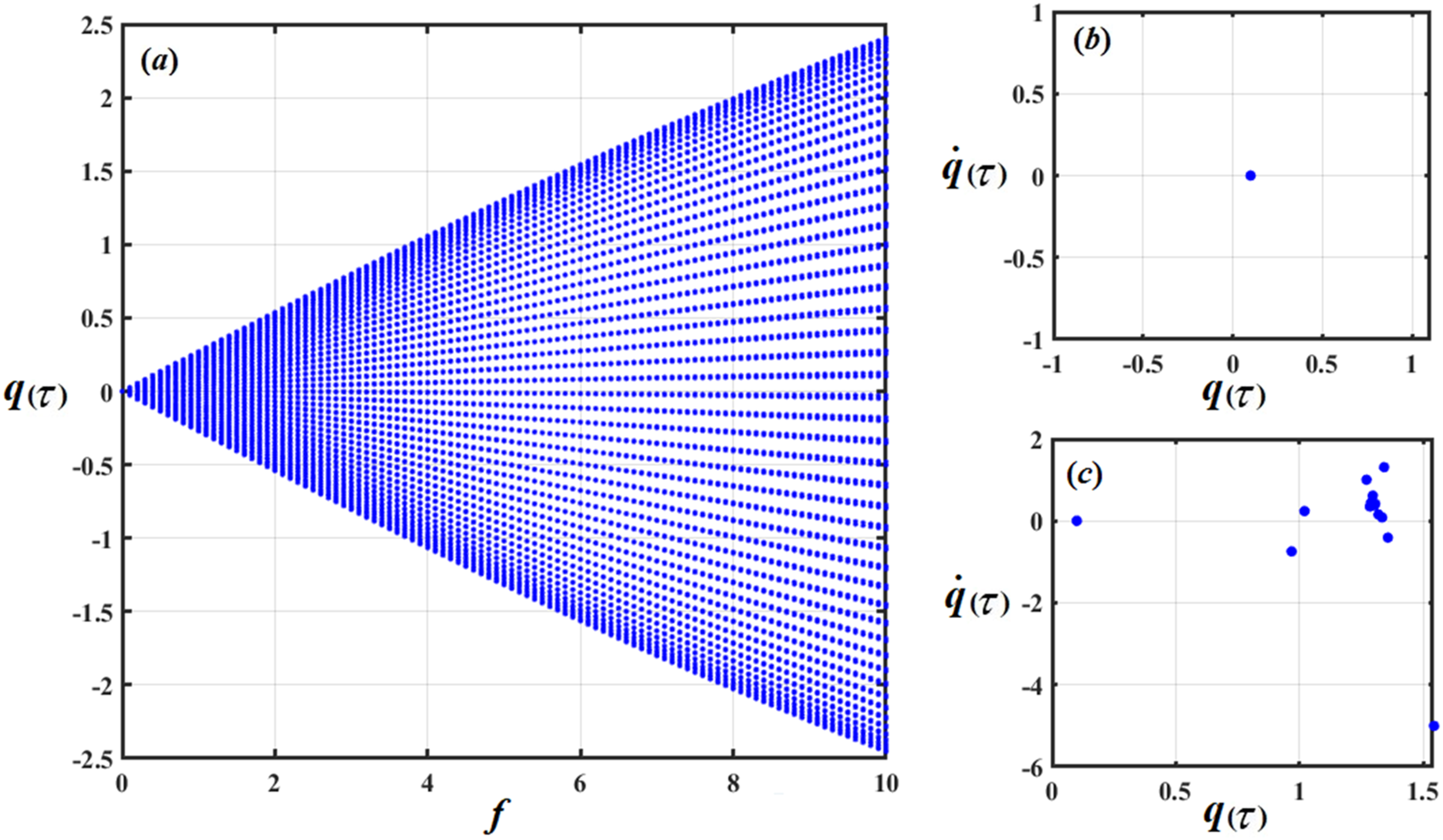
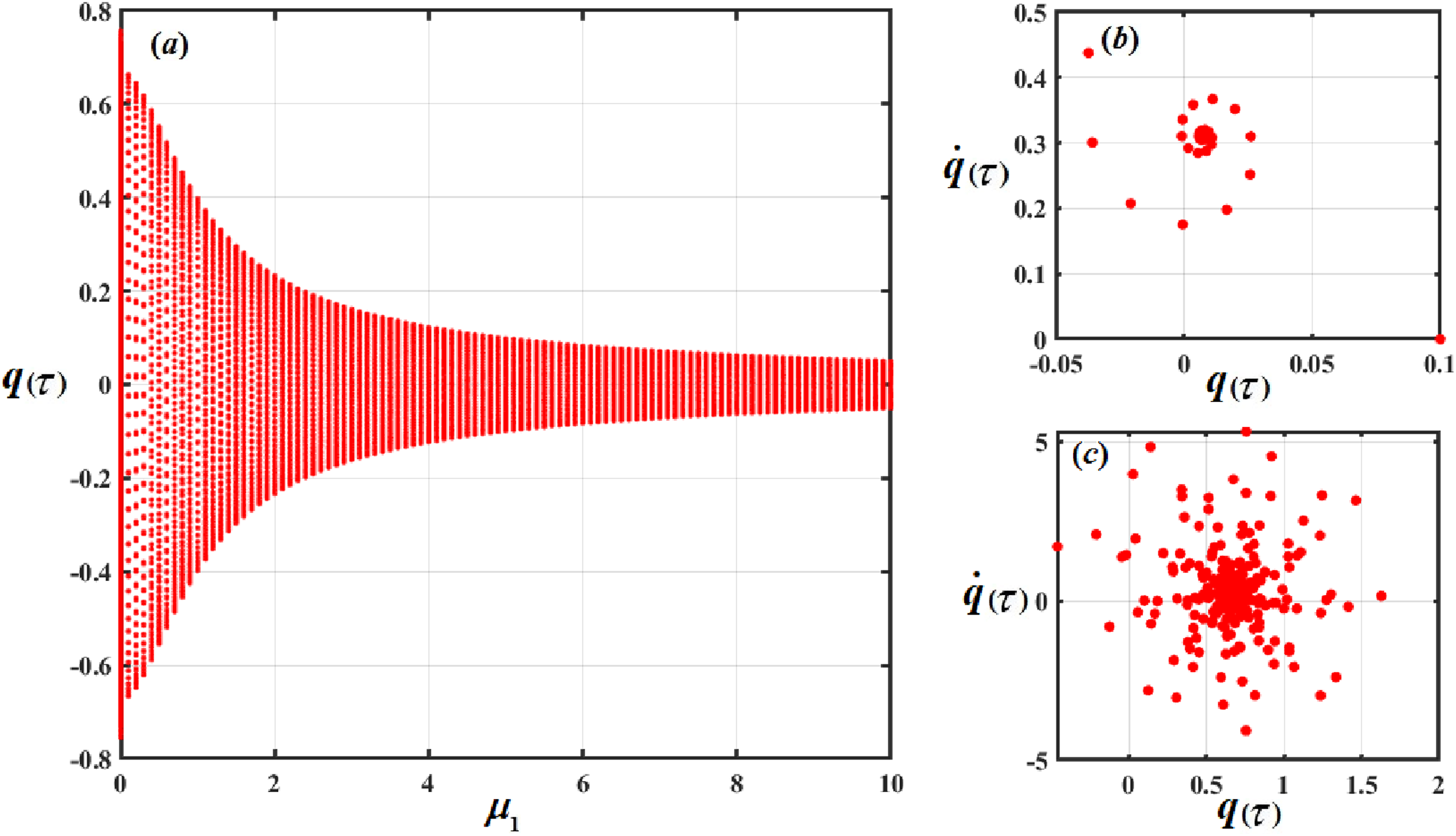
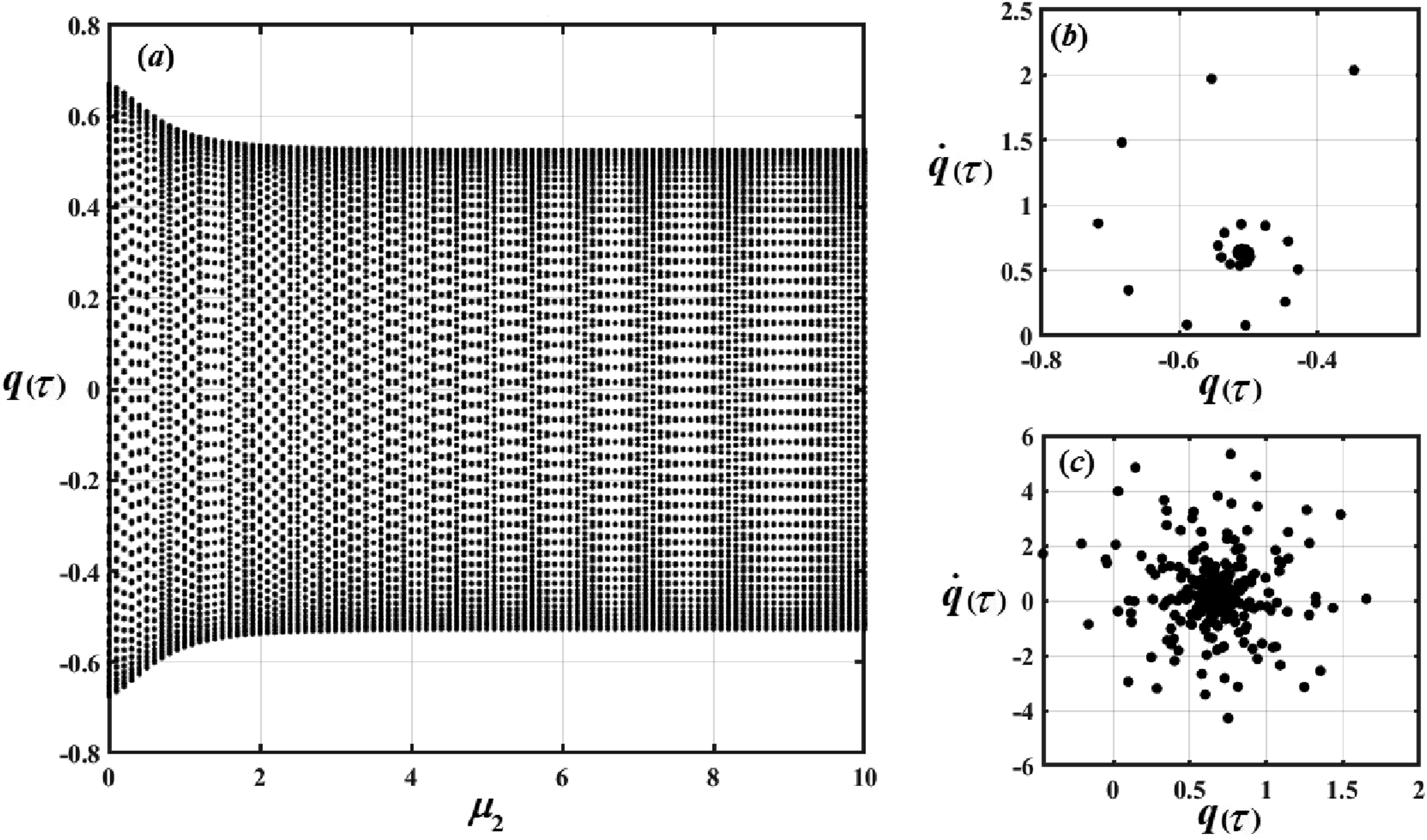
Bifurcation curves graphically depict how a system behaves when a parameter changes. The formation of new equilibrium points or periodic cycles is an instance of a transitional phase in the system’s behavior that they identify.⁴² The bifurcation charts of $q (τ)$ with $f, μ,$ and $μ_{2}$ are shown in Figures 16–18 together with Poincare’ maps at various values of $f, μ,$ and $μ_{2}$ show characteristics of different motion kinds. The excitation amplitude $f$ has periods, as shown in the diagram in Figure 16(a), and each period indicates a distinct type of motion for the system. We noticed that the system moves periodically at $f \in [0, 3]$ , but in the period at $f \in (3, 10)$ , the motion is chaotic. To study the various motions of the system, the drawn figures are presented for different values of $f$ . Figure 16(b), we analyze the case of $f = 0.0005$ , where the blue-dot pattern in the Poincaré map closely resembles a single point, reinforcing the earlier conclusion about the system’s periodic motion. Conversely, at $f = 5$ , as shown in Figure 16(c), the system enters a chaotic state, causing the blue dots to disperse randomly. The damping coefficient $μ_{1}$ exhibits periodic behavior, as shown in Figure 17(a), with each period corresponding to a distinct type of system motion. The system displays chaotic motion for $μ_{1} \in [0, 4]$ , while for $μ_{1} \in (4, 10)$ , the motion is periodic. In Figure 17(b), We examine $μ_{1} = 8$ , where the red-dot pattern in the Poincaré map closely resembles a spiral curve, supporting the previous conclusion about the system’s periodic motion. On the other hand, at $μ_{1} = 0.03$ , as seen in Figure 17(c), the system transformed into a chaotic state, causing the red dots to diverge randomly. The damping coefficient $μ_{2}$ has periods, as shown in the diagram in Figure 18(a), and ever y stage denotes a different kind of system motion. The system is moving chaotically, as we noticed at $μ_{2} \in [0, 3]$ . For the period at $μ_{2} \in (3, 10)$ , the system moves periodically. We analyze the value $μ_{2} = 8$ in Figure 18(b), the Poincaré map’s black-dot pattern closely matches a spiral curve, confirming the earlier finding of the system’s periodic motion. Due to the chaotic state that appears for specific $μ_{2}$ values, the black dots at $μ_{2} = 0.0005$ in Figure 18(c) are randomly distributed.

Figure 16.

(a) Bifurcation diagram of $q (τ)$ with the amplitude $f$ , (b) and (c) Poincaré maps of $q (τ)$ at $f = 0.0005$ and $f = 5,$ respectively.

Figure 17.

(a) Bifurcation diagram of $q (τ)$ with the damping coefficient $μ_{1}$ , (b) and (c) Poincaré maps of $q (τ)$ at $μ_{1} = 8$ and $μ_{1} = 0.03,$ respectively.

Figure 18.

(a) Bifurcation diagram of $q (τ)$ with the damping coefficient $μ_{2}$ , (b) and (c) Poincaré maps of $q (τ)$ at $μ_{2} = 8$ and $μ_{2} = 0.0005,$ respectively.

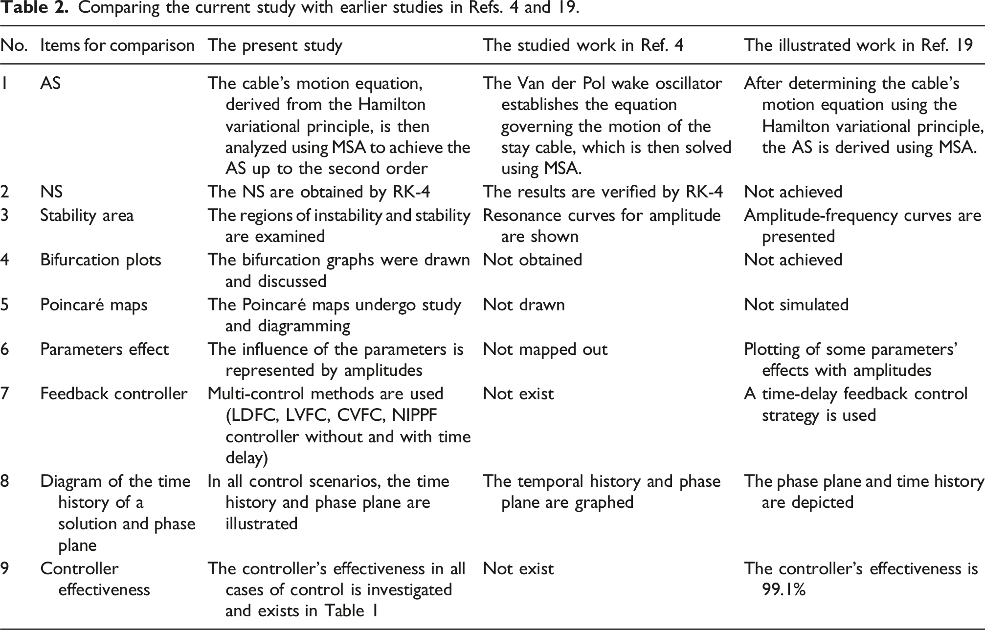
Note that the benchmark work is compared to other previous efforts, including Refs. 4 and 19 in Table 2. These comparisons cover the derived solutions AS, NS, stability regions, bifurcation diagrams, Poincaré maps, parameters effect on the amplitude, feedback controller, and diagram of the time history of a solution and phase plane, and controller effectiveness.

Table 2.

Comparing the current study with earlier studies in Refs. 4 and 19.

No.	Items for comparison	The present study	The studied work in Ref. 4	The illustrated work in Ref. 19
1	AS	The cable’s motion equation, derived from the Hamilton variational principle, is then analyzed using MSA to achieve the AS up to the second order	The Van der Pol wake oscillator establishes the equation governing the motion of the stay cable, which is then solved using MSA.	After determining the cable’s motion equation using the Hamilton variational principle, the AS is derived using MSA.
2	NS	The NS are obtained by RK-4	The results are verified by RK-4	Not achieved
3	Stability area	The regions of instability and stability are examined	Resonance curves for amplitude are shown	Amplitude-frequency curves are presented
4	Bifurcation plots	The bifurcation graphs were drawn and discussed	Not obtained	Not achieved
5	Poincaré maps	The Poincaré maps undergo study and diagramming	Not drawn	Not simulated
6	Parameters effect	The influence of the parameters is represented by amplitudes	Not mapped out	Plotting of some parameters’ effects with amplitudes
7	Feedback controller	Multi-control methods are used (LDFC, LVFC, CVFC, NIPPF controller without and with time delay)	Not exist	A time-delay feedback control strategy is used
8	Diagram of the time history of a solution and phase plane	In all control scenarios, the time history and phase plane are illustrated	The temporal history and phase plane are graphed	The phase plane and time history are depicted
9	Controller effectiveness	The controller’s effectiveness in all cases of control is investigated and exists in Table 1	Not exist	The controller’s effectiveness is 99.1%

Conclusion

A dynamic model of a hanging wire under both static and dynamic stress conditions is discussed in this paper. The NIPPFC with a time delay is used to improve stability and lessen unwanted vibrations, especially in the resonance zone. The HVA is used to build the DE for a hanging cable. The MSA is used to solve this equation up to the second order to obtain the AS. The correctness of the AS is verified by contrasting it with the calculated NS using the RK-4. Solvability requirements and resonance cases are examined to acquire the ME. The solutions’ time histories and frequency responses are graphically represented using MATLAB and Wolfram Mathematica 13.2. Moreover, the time histories of the derived solutions are visually compared in both controlled and uncontrolled cases. Additionally, stability analysis and steady-state solutions are discussed using resonance curves. To determine the critical parameters that result in qualitative changes in the behavior of the system, the nonlinear dynamics of the model are further examined using bifurcation analysis and represented using bifurcation diagrams. Periodic and chaotic oscillations are studied using the Poincaré map, which sheds light on the long-term stability of the system and the appearance of chaotic dynamics. The amplitude of $q (τ)$ was found to be reduced by 47.4%, 87.5%, 89.5%, 92.1%, 97.26%, 99.44%, and 99.39%, respectively, as a consequence of the LDFC, LVFC, CVFC, NIPPF controller without delay $(T = 0)$ , NIPPFC with delay $(T = 0.0015)$ , NIPPFC with $(T = 0.004)$ , and NIPPFC with $(T = 0.008)$ . We observe that the NIPPFC with $(T = 0.004)$ is the best controller for this system. This model is commonly employed in the investigation and creation of flexible structures, including cable-supported systems, transmission lines, and suspension bridges. Additionally, it aids engineers in analyzing how static and dynamic forces like weight, earthquakes, storms, or movement loads affect buildings. It prevents structural instability or failure by anticipating crucial behaviors like vibrations, deflections, or resonance using displacement monitoring. Additionally, it helps with vibration optimization and control to enhance performance and safety. Future research will focus on extending the proposed NIPPFC to large-scale structures such as suspension bridges, incorporating distributed sensors and actuators. Additional efforts will address energy efficiency, robustness under environmental disturbances, and sensitivity to parameter variations. Real-time chaos detection mechanisms and adaptive gain tuning will also be explored. Finally, experimental validation for the obtained results is provided.

Footnotes

ORCID iDs

T. S. Amer

Mohamed K. Abohamer

Author Contributions

Taher A. Bahnasy: Investigation, Methodology, Corroboration, Validation, Data duration, Examination, Visualization, and Reviewing.

Tarek S. Amer: Resources, Conceptualization, Formal analysis, Methodology, Validation, and Reviewing.

Abdel Karim S. Elameer: Formal analysis, Investigation, Methodology, Writing-Original draft preparation, Visualization, and Reviewing.

Mohamed K. Abohamer: Conceptualization, Methodology, Validation, Examination, Corroboration, Reviewing, and Editing.

Funding

The authors received no financial support for the research, authorship, and/or publication of this article.

Declaration of conflicting interests

The authors declared no potential conflicts of interest with respect to the research, authorship, and/or publication of this article.

Data Availability Statement

The datasets used and/or analyzed during the current study available from the corresponding author on reasonable request.*

Appendix

J_{11} = \frac{\partial {\dot{a}}_{1}}{\partial a_{1}} = - 0.5 μ_{1} - \frac{0.5 k_{2} k_{4}}{μ_{3}^{2} + ω_{1}^{2}}, J_{12} = \frac{\partial {\dot{a}}_{1}}{\partial θ_{1}} = \frac{f_{1} {\cos θ}_{1}}{2 ω_{1}}, J_{13} = \frac{\partial {\dot{a}}_{1}}{\partial a_{2}} = \frac{k_{1} \cos (ω_{2} T) {\sin θ}_{2}}{2 ω_{1}}

- \frac{k_{1} \sin (ω_{2} T) {\cos θ}_{2}}{2 ω_{1}}, J_{14} = \frac{\partial {\dot{a}}_{1}}{\partial θ_{2}} = \frac{a_{2} k_{1} \cos (ω_{2} T) {\cos θ}_{2}}{2 ω_{1}} + \frac{a_{2} k_{1} \sin (ω_{2} T) {\sin θ}_{2}}{2 ω_{1}},

J_{21} = \frac{\partial {\dot{θ}}_{1}}{\partial a_{1}} = - \frac{9}{8} ρ a_{1} + \frac{σ_{1}}{a_{1}} + \frac{0.5 k_{2} k_{4} μ_{3}}{a_{1} (μ_{3}^{2} + ω_{1}^{2})}, J_{22} = \frac{\partial {\dot{θ}}_{1}}{\partial θ_{1}} = \frac{f_{1} {\sin θ}_{1}}{2 a_{1} ω_{1}},

J_{23} = \frac{\partial {\dot{θ}}_{1}}{\partial a_{2}} = \frac{k_{1} \cos (ω_{2} T) {\cos θ}_{2}}{2 ω_{1} a_{1}} + \frac{k_{1} \sin (ω_{2} T) {\sin θ}_{2}}{2 ω_{1} a_{1}},

J_{24} = \frac{\partial {\dot{θ}}_{1}}{\partial θ_{2}} = - \frac{k_{1} a_{2} \cos (ω_{2} T) {\sin θ}_{2}}{2 ω_{1} a_{1}} + \frac{k_{1} a_{2} \sin (ω_{2} T) {\cos θ}_{2}}{2 ω_{1} a_{1}},

J_{31} = \frac{\partial {\dot{a}}_{2}}{\partial a_{1}} = - \frac{k_{3} \cos (ω_{1} T) {\sin θ}_{2}}{2 ω_{2}} - \frac{k_{3} \sin (ω_{1} T) {\cos θ}_{2}}{2 ω_{2}},

J_{32} = \frac{\partial {\dot{a}}_{2}}{\partial θ_{1}} = 0, J_{33} = \frac{\partial {\dot{a}}_{2}}{\partial a_{2}} = - 0.5 μ_{2}, J_{34} = \frac{\partial {\dot{a}}_{2}}{\partial θ_{2}} = - \frac{k_{3} a_{1} \cos (ω_{1} T) {\cos θ}_{2}}{2 ω_{2}}

+ \frac{k_{3} a_{1} \sin (ω_{1} T) {\sin θ}_{2}}{2 ω_{2}}, J_{41} = \frac{\partial {\dot{θ}}_{2}}{\partial a_{1}} = - \frac{3 ρ a_{1}}{4} - \frac{f_{1} {\cos θ}_{1}}{2 a_{1}^{2} ω_{1}}

- \frac{k_{1} a_{2} \cos (ω_{2} T) {\cos θ}_{2}}{2 a_{1}^{2} ω_{1}} - \frac{k_{1} a_{2} \sin (ω_{2} T) {\sin θ}_{2}}{2 a_{1}^{2} ω_{1}} - \frac{k_{3} \cos (ω_{1} T) {\cos θ}_{2}}{2 a_{2} ω_{2}}

+ \frac{k_{3} \sin (ω_{1} T) {\sin θ}_{2}}{2 a_{2} ω_{2}}, J_{42} = \frac{\partial {\dot{θ}}_{2}}{\partial θ_{1}} = - \frac{f_{1} {\sin θ}_{1}}{2 a_{1} ω_{1}}, J_{43} = \frac{\partial {\dot{θ}}_{2}}{\partial a_{2}} = - \frac{3 ρ a_{1}^{2}}{8 a_{2}}

+ \frac{σ_{2}}{a_{2}} + \frac{f_{1} {\cos θ}_{1}}{2 a_{1} a_{2} ω_{1}} + \frac{k_{1} \cos (ω_{2} T) {\cos θ}_{2}}{a_{1} ω_{1}} + \frac{k_{1} \sin (ω_{2} T) {\sin θ}_{2}}{a_{1} ω_{1}} + \frac{0.5 k_{2} k_{4} μ_{3}}{a_{2} (μ_{3}^{2} + ω_{1}^{2})},

J_{44} = \frac{\partial {\dot{θ}}_{2}}{\partial θ_{2}} = - \frac{k_{1} a_{2} \cos (ω_{2} T) {\sin θ}_{2}}{2 a_{1} ω_{1}} + \frac{k_{1} a_{2} \sin (ω_{2} T) {\cos θ}_{2}}{2 a_{1} ω_{1}} + \frac{k_{3} a_{1} \cos (ω_{1} T) {\sin θ}_{2}}{2 a_{2} ω_{2}} + \frac{k_{3} a_{1} \sin (ω_{1} T) {\cos θ}_{2}}{2 a_{2} ω_{2}} .

References

Huang

Chen

. Cable structures in bridge engineering. J Bridge Eng 2019; 24(8): 02019001.

Gimsing

Georgakis

. Cable supported bridges: concept and design. John Wiley & Sons Ltd., 2012.

Agrawal

Fujino

Bhartia

. Instability due to time delay and its compensation in active control of structures. Earthq Eng Struct Dynam 1993; 22(3): 211–224.

Cong

Jiang

Kang

, et al. Nonlinear dynamic analysis of vortex-induced resonance of a flexible cable. Nonlinear Dyn 2023; 112(2): 793–810.

Deng

Huang

, et al. Experimental investigation on aerodynamic interference of two kinds of suspension bridge hangers. J Fluid Struct 2019; 90: 57–70.

Deng

Chen

. Unsteady theoretical analysis on the wake-induced vibration of suspension bridge hangers. J Bridge Eng 2018; 24(2): 04018113.

Rega

. Nonlinear vibrations of suspended cables—Part I: modeling and analysis. Appl Mech Rev 2004; 57(6): 443–478.

Rega

. Nonlinear vibrations of suspended cables—Part II: deterministic phenomena. Appl Mech Rev 2004; 57(6): 479–514.

Ibrahim

. Nonlinear vibrations of suspended cables—Part III: random excitation and interaction with fluid flow. Appl Mech Rev 2004; 57(6): 515–549.

10.

Ugli Shakirov

Ugli Khudoyberdiyev

Achilov

. A suspension bridge as one of modern prospective type of construction. Ares 2022; 3(2): 13–17.

11.

Zhang

, et al. An improved analytical algorithm on main cable system of suspension bridge. Appl Sci 2018; 8(8): 1358.

12.

Lepidi

Gattulli

. Static and dynamic response of elastic suspended cables with thermal effects. Int J Solid Struct 2012; 49(9): 1103–1116.

13.

Huang

. Review of the main cable shape control of the suspension bridge. Appl Sci 2023; 13(5): 3106.

14.

Wang

Hua

Wang

, et al. Mechanical behavior of magnetorheological dampers after long-term operation in a cable vibration control system. Struct Control Health Monit 2019; 26(1): e2280.

15.

Wang

Schaechter

. Dynamics of controlled mechanical systems with delayed feedback. Appl Mech Rev 2003; 56(3): 37.

16.

Peng

Xia

Sun

, et al. Stability in parametric resonance of a controlled stay cable with time delay. Int J Struct Stabil Dynam 2024; 24(21): 2450233.

17.

Liu

Olgac

Cheng

. Delayed resonator with multiple distributed delays-considering and optimizing the inherent loop delay. J Sound Vib 2024; 576: 118290.

18.

Zhu

Xiao

Huang

, et al. Spatiotemporal dynamics optimization of a delayed reaction-diffusion mussel-algae model based on PD control strategy. Chaos Solitons Fractals 2023; 173: 113751.

19.

Peng

, et al. Time-delay feedback control of a suspended cable driven by subharmonic and superharmonic resonance. Chaos Solitons Fractals 2024; 181: 114646.

20.

Zhao

Huang

Chen

, et al. Nonlinear vibration behaviors of suspended cables under two-frequency excitation with temperature effects. J Sound Vib 2018; 416: 279–294.

21.

Warminski

Zulli

Rega

, et al. Revisited modelling and multimodal nonlinear oscillations of a sagged cable under support motion. Meccanica 2016; 51(11): 2541–2575.

22.

Tang

. Subharmonic and homoclinic solutions for second order Hamiltonian systems with new superquadratic conditions. Chaos Solitons Fractals 2015; 73: 183–190.

23.

Tang

Peng

, et al. Vibration control of nonlinear vibration of suspended cables based on quadratic delayed resonator. J Phys : Conf Ser 2020; 1545(1): 012005.

24.

Mirhashemi

Haddadpour

. Nonlinear dynamics of a nearly taut cable subjected to parametric aerodynamic excitation due to a typical pulsatile wind flow. Int J Eng Sci 2023; 188: 103865.

25.

Sun

Zhou

. Nonlinear responses of suspended cable under phase-differed multiple support excitations. Nonlinear Dyn 2021; 104(2): 1097–1116.

26.

Bahnasy

Amer

Abohamer

, et al. Stability and bifurcation analysis of a 2DOF dynamical system with piezoelectric device and feedback control. Sci Rep 2024; 14: 26477.

27.

Amer

Bahnasy

Abosheiaha

, et al. The stability analysis of a dynamical system equipped with a piezoelectric energy harvester device near resonance, 2024; 44(1): 382–410.

28.

Amer

Bahnasy

. Duffing oscillator’s vibration control under resonance with a negative velocity feedback control and time delay. Sound Vib 2021; 55(3): 191–201.

29.

Amer

Bahnasy

Almahalawy

. Vibration analysis of permanent magnet motor rotor system in shearer semi-direct drive cutting unite with speed controller and multi-excitation forces. AMIS 2021; 3: 373–381.

30.

Amer

Starosta

Almahalawy

, et al. The stability analysis of a vibrating auto-parametric dynamical system near resonance. Appl Sci 2022; 12(3): 1737.

31.

Amer

Arab

Galal

. On the influence of an energy harvesting device on a dynamical system. Control 2024; 43(2): 669–705.

32.

Bek

Amer

Almahalawy

, et al. The asymptotic analysis for the motion of 3DOF dynamical system close to resonances. Alex Eng J 2021; 60: 3539–3551.

33.

Amer

Starosta

Elameer

, et al. Analyzing the stability for the motion of an unstretched double pendulum near resonance. Appl Sci 2021; 11(20): 9520.

34.

Tian

Shen

Chen

, et al. Discovery potential for heavy neutral leptons with displaced vertices at the LHC. Mod Phys Lett A 2025; 39: 2450223.

35.

Moussa

Youssouf

Wassiha

, et al. Homotopy perturbation method to solve Duffing–Van der Pol equation. Adv Differ Equ Control Process 2024; 31: 299–315.

36.

Alsolami

. A good initial guess for approximating nonlinear oscillators by the homotopy perturbation method. FU Mech Eng 2023; 21: 021–029.

37.

Alshomrani

Alharbi

Alanazi

, et al. Homotopy perturbation method for solving a nonlinear system for an epidemic. Adecp 2024; 31: 347–355.

38.

Imran

Zeemam

Basit

, et al. Exploration of stagnation-point flow of Reiner–Rivlin fluid originating from the stretched cylinder for the transmission of the energy and matter. Sci Rep 2025; 15: 6515.

39.

Chaudhry

Basit

Akhtar

, et al. Computational heat and mass transfer analysis of magnetized nanofluid flow under the influences of motile microorganisms and thermal radiation. Mod Phys Lett B 2025; 39: 2350111.

40.

Basit

Bashir

Imran

, et al. Analysis of efficient partial differential equations model for nano-fluid flow through wedge involving minimal energy and thermal radiation. J Radiat Res Appl Sci 2025; 18: 101331.

41.

Basit

Imran

Anwar-Ul-Haq

, et al. Advancing renewable energy systems: a numerical approach to investigate nanofluidics’ role in engineering involving physical quantities. Sci Rep 2025; 15: 261.

42.

Bahnasy

Amer

Almahalawy

, et al. A chaotic behavior and stability analysis on quasi-zero stiffness vibration isolators with multi-control methodologies, J Low Freq Noise Vib Act Control 2025; 44, 1094, 1116.

Chaotic behavior analysis of a hanging wire system with NIPPFC controller

Abstract

Keywords

Introduction

Investigation of the dynamical system mathematically

The suggested strategy and resonance categorization

Steady-state strategies and analyzing stability

Results and discussion

Conclusion

Footnotes

ORCID iDs

Author Contributions

Funding

Declaration of conflicting interests

Data Availability Statement

Appendix

References