Sage Journals: Discover world-class research

Abstract

Monitoring pipeline infrastructure is essential for ensuring safety, efficiency, and environmental sustainability in energy transportation. External disturbances, such as knocking and drilling, are common challenges that can impact pipeline integrity. The proposed approach develops a multimodal framework for detecting and localizing external disturbances in oil and gas pipelines by integrating statistical methods, signal processing, and advanced diagnostics. The experimental study was conducted on pipelines under three conditions: healthy, knocking, and drilling to assess the capability of the framework to detect and localize external disturbances. The proposed approach effectively classified pipeline conditions. External disturbance localization was precise for knocking disturbances due to their distinct high-frequency characteristics. However, drilling localization was challenging with the current experimental setup. Drilling generated low-frequency vibrations with longer wavelengths, reducing energy loss and broader time responses across closely spaced nodes in the 2-meter pipe setup. This behavior provides insight into the spatial arrangement of the optimal node spacing for effective localization of low-frequency disturbances in long-range pipeline systems.

Keywords

detection external disturbance localization oil and gas pipeline statistical analysis

Introduction

Pipelines are essential links of the energy sectors for the transportation and distribution of bulk energy products from one part of the country to another and from refineries to terminals. These cross-country pipelines pass through diverse terrains such as city outskirts, villages, rivers, remote lands, and challenging landscapes, making them vulnerable targets for external disturbance. External disturbances are referred to as any action that obstructs, damages, or tampers with the oil and gas pipelines. These intentional or unintentional actions can compromise the system’s integrity and may lead to damage or failure. The term also includes activities such as theft, tapping, knocking, drilling, or other forms of sabotage.

These high and rising value of the transported products are becoming lucrative targets, including attempts to tap for illegal extraction. The sabotage of the pipeline has serious implications and causes major risks to humans and the environment. Despite the efforts of oil and gas companies, the incident of external disturbance persists and raise concerns about the safety and reliability of the pipeline. Corrosion and external interference remain the leading causes of pipeline damage incidents.^1–3 External disturbances, particularly third-party interference, are frequently cited as the primary contributors to pipeline failures.^4–7 In Nigeria, pipelines and related facilities were repeatedly attacked, which caused great loss of life and property. The Nigerian National Petroleum Corporation (NNPC) documented huge cases of vandalism between 2000 and 2008.

Table 1 outlines historical incidents of external interference in oil and gas pipelines, including theft, vandalism, tampering, and sabotage. It summarizes the types of interference, impacts, and consequences as documented in various studies.

Table 1.

Incidents of external interference in oil and gas pipelines.

Incident and location	Type of interference	Impact and consequences
Balticconnector pipeline damage (2023) Baltic sea⁸	Anchor dragging (suspected deliberate damage to subsea cables and pipelines)	Energy supply disruption, infrastructure, and physical damage
Nord stream pipeline sabotage (2022) Baltic sea⁹	Sabotage (explosives)—deliberately ruptured Nord Streams 1 and 2	Gas leakage, environmental disturbance, impact on human lives and infrastructure
Transnet pipeline theft incident (2020) South Africa¹⁰	Tampering–illegal tapping	Leakage, massive fuel spillage, environmental damage, toxic exposure
Pemex pipeline explosion (2019) Mexico¹¹	Stealing gasoline from the pipeline	Pipeline rupture and explosion, fatalities, injuries
Oil spill incidents and pipeline vandalism (1970 and 2006) Nigeria^12,13	Vandalism, theft, and unauthorized tapping	Fatalities, injuries, environmental devastation, contamination of potable water sources (streams, rivers)

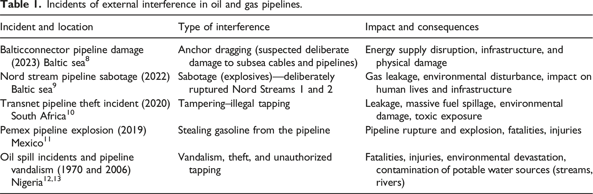
The problem is receiving considerable attention in the energy sectors because of the threats and vulnerability of their long-distance pipeline networks. The ability to predict the pipeline against external disturbance is valuable knowledge in the industries. Hence, there is a need for reliable pipeline monitoring technology for fault detection and localization.

Pipeline monitoring technologies have seen significant advancements in fault detection,^14–18 localization,^19–22 and structural health monitoring.^23–26 Table 2 provides a synthesis of recent advances, key contributions, and research gaps identified in the literature on pipeline monitoring, leak detection, and fault localization. The table highlights the progress made and addresses the challenges identified in the most relevant studies discussed in the field.

Table 2.

Recent advances, contributions, and research gaps in pipeline monitoring, leak detection, and fault localization.

Area	Key contributions	Identified research gaps
Recent advances and reviews on Pipeline inspection, leak detection, and monitoring technologies^27–29	- Discussed advances in leakage detection and localization methods in pipeline systems - Covers commonly used subsea inspection and monitoring technologies, along with recent developments and trends.	- Each technique has some merits and drawbacks. - Real-time intelligent leak detection systems are needed. - Monitoring of oil and gas pipeline networks using efficient wireless communications technology can be more beneficial.
Fault detection and localization in pipeline monitoring	- Development and analysis of a distributed leak detection and localization system for crude oil pipelines.³⁰ - Reviews global developments in pipeline robot localization techniques.³¹	- Fault localization is critical in pipeline monitoring. - Current limitations in pipeline robot localization technologies need addressing. - Future research should focus on system performance analysis under various failures and utilize sensor fusion and data-centric frameworks for accurate fault detection.³²
Advanced techniques (AI, IoT, machine learning)	- Implemented to enable real-time monitoring of pipeline operations through the Internet of Things (loT) platform.³³ - AI-based pipe leakage detection using AE signals³⁴ - Data-driven multi-fault detection using artificial neural networks³⁵ - Integration of data-driven techniques for monitoring and assessment of pipelines.¹⁷	- Challenges persist in the deployment of industrial IoT-based solutions. - Real-time data analysis using machine learning algorithms for anomaly detection. - Lack of large-scale datasets for training AI models. - Energy-efficient IoT devices for remote monitoring remain a challenge.

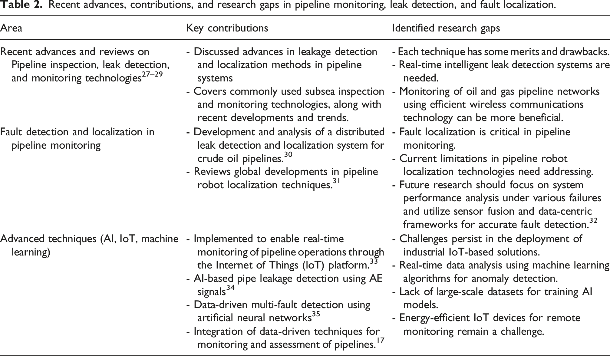
Signal processing techniques have also been extensively explored. A monitoring method³⁶ based on the vibration signals obtained from the pipe in its healthy and flawed states was used and was further processed through the Hilbert–Huang transform (HHT) and its associated signal decomposition technique, empirical mode decomposition (EMD). The EMD decomposes the vibration signals into a series of intrinsic mode functions (IMFs). Damage-sensitive parameters, such as damage index EM-EDI evaluate the deviation in structural integrity. Leak localization³⁷ has been achieved through empirical mode decomposition and cross-correlation (EMD-CC), which adaptively extracts effective leak signals and significantly improves localization accuracy.

Despite these advancements in pipeline monitoring and fault detection, several challenges are still present. Many existing studies focus on fault detection and localization with limited integration of multimodal approaches. Monitoring techniques are often constrained by their limited applicability in real-world dynamic conditions. Moreover, unprocessed or improperly processed signals may lead to inaccurate conclusions. Pipeline monitoring and fault detection systems have traditionally employed individual methods, which are often insufficient to address the complexities of real-time conditions. These approaches lack the necessary integration to analyze dynamic pipeline response comprehensively. The application of the multimodal approach remains limited in pipeline monitoring research. Real-time signals from pipelines generate large datasets that are difficult to analyze efficiently. A critical challenge is to isolate the faulty signals for quick and reliable decision-making. Partial-model-based damage identification using stiffness separation techniques has demonstrated effective strategies for structural health monitoring in long-span steel truss bridges by significantly reducing computation time.³⁸ This approach detects the damage using only partial structural information and depends on the partial model information. Similarly, the stiffness separation method has been applied to large-scale space truss structures to simplify the high-dimensional damage identification problem.³⁹ This method treats displacement responses as additional boundary conditions, and the truss structure is divided into smaller substructures. This reduces both the analytical model size and the number of unknown parameters.

Our proposed methodology introduces a multimodal framework that integrates statistical analysis (ANOVA and post-hoc tests), signal decomposition (EMD), wavelet analysis, cross-correlation, and damage index computation. Each method addresses specific challenges. This approach reduces the computational load and accelerates the prediction process for real-time applications. The proposed method is more generalizable, covering diverse pipeline conditions and external disturbance scenarios. This approach will also provide insight into the nature of commonly observed external disturbance and its associated pattern through an experimental data-driven multimodal approach.

In our experimental setup, vibration signals are collected from a pipeline under various controlled disturbances. The collected signals are relatively simple, with peaks occurring at random times and locations in response to knocking or external excitation designed to simulate the effect of intermittent events that might occur in the field, such as drilling, vandalism, or theft. Although the experimental signals are straightforward, they describe how each step of our approach can effectively detect these disturbances and validate the algorithms in a clear and controlled manner. Real-world signals in pipelines are often complex, continuous, and affected by a mix of noise, environmental interferences, and operational vibrations. This makes anomaly detection more challenging. Our methodology demonstrates a comprehensive, layered process that is sufficiently secure simple experimental signals and compatible with handling the complexities of real-time monitoring in practical applications. This step-by-step approach effectively filters, analyses, and validates signals, ensuring that the algorithms work reliably even under the more challenging, noisy conditions encountered in real-life pipeline environments. The flow chart (Figure 1) covers the step-by-step procedure from initial data collection to external disturbance detection and localization. The integration of statistical analysis, EMD, wavelet transform, and cross-correlation forms the core of the proposed framework, and each method plays a specific role in a sequential, complementary manner.

Figure 1.

Flowchart of the multimodal framework for external disturbance detection and localization in pipelines.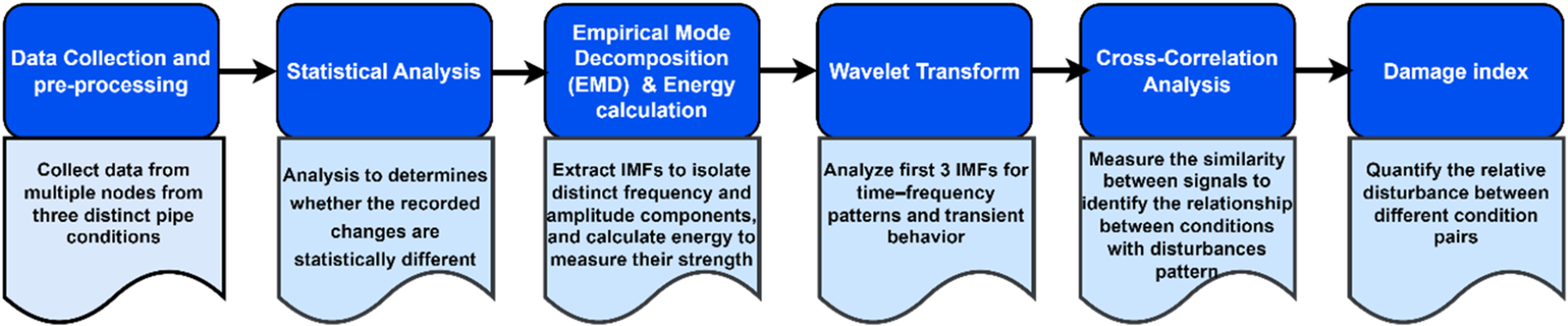

Statistical analysis is first used to confirm whether there are significant differences between signal conditions, such as healthy, knocking, and drilling. EMD then decomposes each signal into IMFs which separate different frequency and amplitude components to isolate the fault features. The continuous wavelet transform (CWT) is applied to the first three IMFs to provide a time–frequency representation, which helps visualize transient features and their evolution over time. Finally, cross-correlation analysis is used to assess similarity between signals recorded for distinct conditions of pipes at different sensor nodes. This step supports the localization of disturbances by capturing how vibrations propagate along the pipeline. These techniques form a robust multimodal framework for detecting and localizing external pipeline disturbances.

The paper is organized into five key sections to present the proposed methodology and its implementation systematically. The Introduction section outlines the significance of pipeline monitoring, highlights existing challenges, and identifies the need for a multimodal approach. Section 2 explores the governing equations and transient effects on pipeline dynamics to provide a theoretical foundation to understand pipeline responses under external forces such as knocking and drilling. Section 3 describes experimental data acquisition and a data-driven multimodal approach for detecting and localizing external disturbances in pipelines. Section 4 focuses on a data-driven multimodal approach to identify external disturbances in pipelines by processing signals from three conditions (healthy, knocking, and drilling) using statistical analysis, EMD, wavelet analysis, and cross-correlation techniques. Finally, Section 5 extends this framework to localize external disturbances by analyzing node-specific signals from four accelerometer locations.

Before implementing this detection approach, it is essential to understand the nature of various external disturbances and how the pipeline dynamically responds under transient effects. We use the PDE wave equation to simulate pipeline behavior under external forces. This foundational analysis provides insights into the pipeline’s vibrational response to transient disturbances, which informs the design and effectiveness of the anomaly detection approach.

Governing equations and transient effects on pipeline dynamics under external force

Vibration signals captured from the accelerometers mounted on the pipeline can be modeled as

s (t) = \sum_{i = 1}^{N} a_{i} (t) + η (t)

(1)

where

a_{i} (t)

is the contribution of various vibration sources due to external disturbances, and

η (t)

refers to noise.

External disturbances are often classified as transient events, as these activities induce sudden and temporary forces or disturbances to the pipeline, generating a change in the time-dependent parameters. This is also called short-duration impacts on the pipeline’s behavior. They can generate dynamic loading, which may produce vibration and shocks within the pipeline. These events can alter the vibration pattern, which can be effectively measured using accelerometers. It also simulates the real-world situation that a pipe may experience and provides valuable data for comparison with the actual responses.

The Gaussian function (equation (2)) is the best way to represent the force in transient simulation and effectively model the rise and decay of the transient nature of the real-world impacts.

{f (t)}_{k n o c k i n g} = F_{0} e^{- \frac{{(t - t_{0})}^{2}}{2 σ^{2}}}

(2)

F₀ is the peak magnitude of the force, t₀ is the time at which the force reaches its maximum value, and σ is the standard deviation that controls the width of the Gaussian curve.

The function represents a localized, time-dependent impact at a fixed point along the pipeline. To simulate the knocking effect, a specified number of impacts are defined, with the timing of these impacts randomly generated within the simulation period and magnitudes assigned randomly. This approach effectively simulates varying strengths and timings of hammering events. The equation was used to model the short-lived, transient characteristics of a knocking event at a specific location on the pipeline.

The drilling effect on the pipe can be simulated by periodic or continuous forces that impact the localized area over a period, as drilling applies a repetitive force in a specific direction. A sinusoidal function is applied to capture the oscillatory nature of drilling with a localized spatial context of the drilling point. A suitable equation (equation (3)) can be

{f (x, t)}_{d r i l l i n g} = Asin (ω t) e^{- \frac{x - x_{0}}{2 σ^{2}}}

(3)

A is the amplitude of the force and ω is the angular frequency representing the repetitive nature of drilling. x₀ is a position along the pipe where the drilling occurs. σ controls the spatial spread of the force. A sinusoidal force is applied at a specific location, and the drilling frequency defines the oscillatory behavior, imitating the repetitive drilling motion. Drill amplitude represents the strength of the drilling force. The force decays with the distance, simulating the localized nature of the drilling behavior.

Drilling typically induces the vibration with lower amplitude compared to sudden impacts like hammering or knocking. The amplitude of the drilling depends upon the type of drill being used and the pipeline material and thickness. Knocking causes higher amplitude vibrations due to sudden, localized impact that occurs when the pipe is externally disturbed. Knocking is generally higher peak forces over a short duration.

For modeling the dynamic response of a pipeline subjected to external disturbance, a wave equation is appropriate. The accelerometer captures the mechanical vibration governed by the wave equation (equation (4)).

The general form of the wave equation used to model the pipeline dynamic response is given by:

\frac{\partial^{2} u (x, t)}{\partial t^{2}} - c^{2} \frac{\partial^{2} u (x, t)}{\partial x^{2}} = f (x, t)

(4)

u(x, t) is the displacement of the pipeline at position x and time t, and c is the wave speed.

It is important to emphasize that these numerical simulations do not replicate the actual experimental conditions or data. Instead, the simulations aim to conceptually illustrate how knocking and drilling disturbances manifest dynamically in the pipeline. The intention is to provide a clear understanding of the underlying principles and physical phenomena associated with external interference, serving as a basis for the subsequent experimental and analytical phases.

Experimental data acquisition and data-driven multimodal approach for monitoring and localization of external disturbances in pipelines

Experimental setup for the data acquisition

This section outlines the experimental setup, measurement nodes, and data collection methodology. This experimental framework serves as the foundation for real-time monitoring and assessment of pipeline health.

The experiment is conducted as a part of a data-driven multimodal approach for external disturbance identification and localization in the pipeline. External disturbance, such as tampering events, generates mechanical vibrations that propagate along the pipeline. These vibrations are captured using accelerometers to understand the propagation of the wave generated due to external disturbance. Carbon steel pipes are commonly used in the oil and gas industry due to their desired mechanical properties and inherent corrosion resistance. This study utilized a 2-inch diameter, 6-meter-long carbon steel pipe, a common grade for oil and gas transmission applications. A custom test rig was designed and fabricated specifically for this experiment to explore the proposed external disturbance identification and localization approach.

The 6-meter pipe was cut into three equal sections (each 2 m long), with each section representing a different condition:

• Healthy pipe: The first section (healthy pipe) remained intact and was designated as the baseline reference condition representing the normal operating condition of the pipeline. The signal from this condition of the pipe is referred to as a healthy signal.

• Tampered Pipe: The second section (tampered pipe) was subjected to a series of knocking events, varying in time, magnitude, and location along the pipe, to simulate mechanical tampering. The signal obtained from this condition is referred to as a knocking signal.

• Drilling-affected pipe: The third section, referred to as the drilling-affected section, underwent drilling to replicate external disturbances caused by drilling activities. The signal obtained from this condition is referred to as a drilling-induced signal.

The experimental setup involves pipelines mounted on stands at both ends to facilitate effective data acquisition. Four data collection nodes were mounted along the pipeline. The experimental setup was designed to simulate a controlled pipeline system and to monitor critical parameters and abnormalities along the pipe. In the current lab-scale setup, four nodes are strategically placed to collect accelerometer responses wirelessly. Node 1 and Node 4, positioned approximately 5 cm from each end, served as boundary nodes to capture inlet and outlet conditions, respectively. Node 2 and Node 3 were positioned between them at approximately equal distances, around 63 cm apart from their adjacent nodes. This evenly spaced configuration was selected to monitor wave propagation and energy distribution across multiple points on the pipeline to understand and validate fault detection and localization for external disturbances. One end of the pipeline is equipped to supply pressurized air under controlled conditions via secured fittings to prevent air leaks. This test rig, shown in Figure 2, allows a comprehensive evaluation of how different tampering conditions impact the pipeline’s normal parameters.

Figure 2.

(a) Experimental setup with data collection nodes and (b) sensor integration with Arduino Uno R4.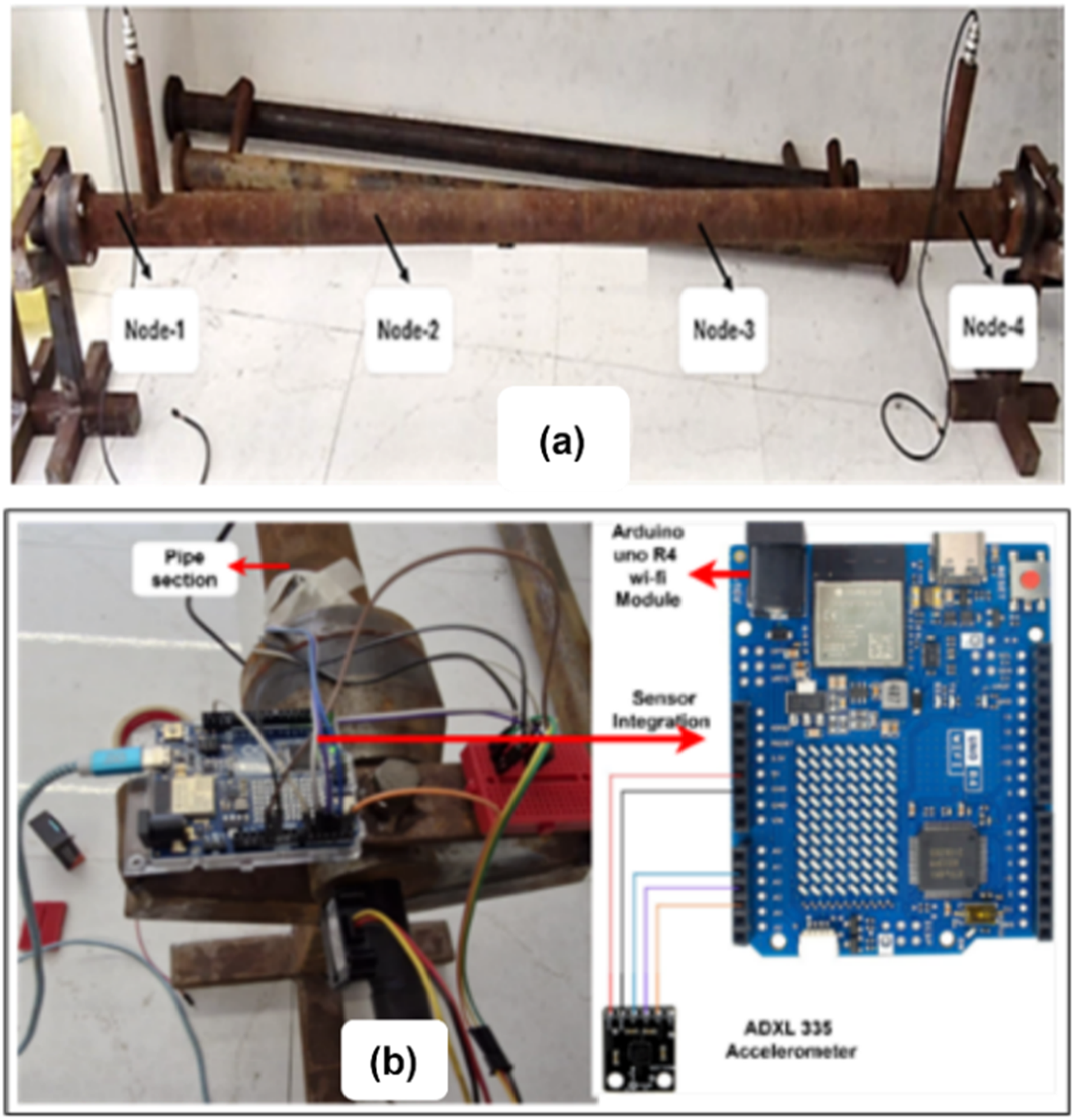

The data collection nodes comprised the ADXL335 accelerometer and Arduino Uno R4 modules, positioned along the pipeline to collect the vibration data. The ADXL335, a MEMS accelerometer, is selected for its low cost, compact size, and ability to measure acceleration across three axes (x, y, and z). Once the stable condition is achieved, the Arduino starts collecting the data from the accelerometer at predetermined intervals.

The ADXL335 accelerometer used in this study has a typical sensitivity of approximately 300 mV/g and a measurement range of ±3 g, making it suitable for detecting both low- and high-frequency vibrations caused by external disturbances. During the experimental phase, the data were collected using an Arduino Uno Wi-Fi module with wireless transmission. For the purpose of detailed time–frequency analysis, such as EMD and CWT, the recorded signals were normalized and post-processed in MATLAB. During this stage, the data were resampled at 1000 Hz to ensure adequate resolution for capturing transient features and preserving the integrity of the original signal.

The acceleration measurements in all three axes were recorded from four nodes under three distinct conditions of the pipe. Real-time monitoring was achieved, and the collected data was transmitted wirelessly to a database for further analysis. After the data collection, the signals were processed through the proposed algorithmic approach.

Data-driven multimodal approach for detection and localization of external disturbances in pipelines

The data-driven multimodal approach presented in Figure 3 is a systematic and effective approach for the detection and localization of external disturbances in oil and gas pipelines. The external disturbance detection algorithm is implemented and outlined step by step in Section 4, as illustrated in Figure 3, while the localization process is implemented and systematically detailed in Section 5.

Figure 3.

Flowchart illustrating the steps of the data-driven multimodal approach for external disturbance identification and localization in the pipeline.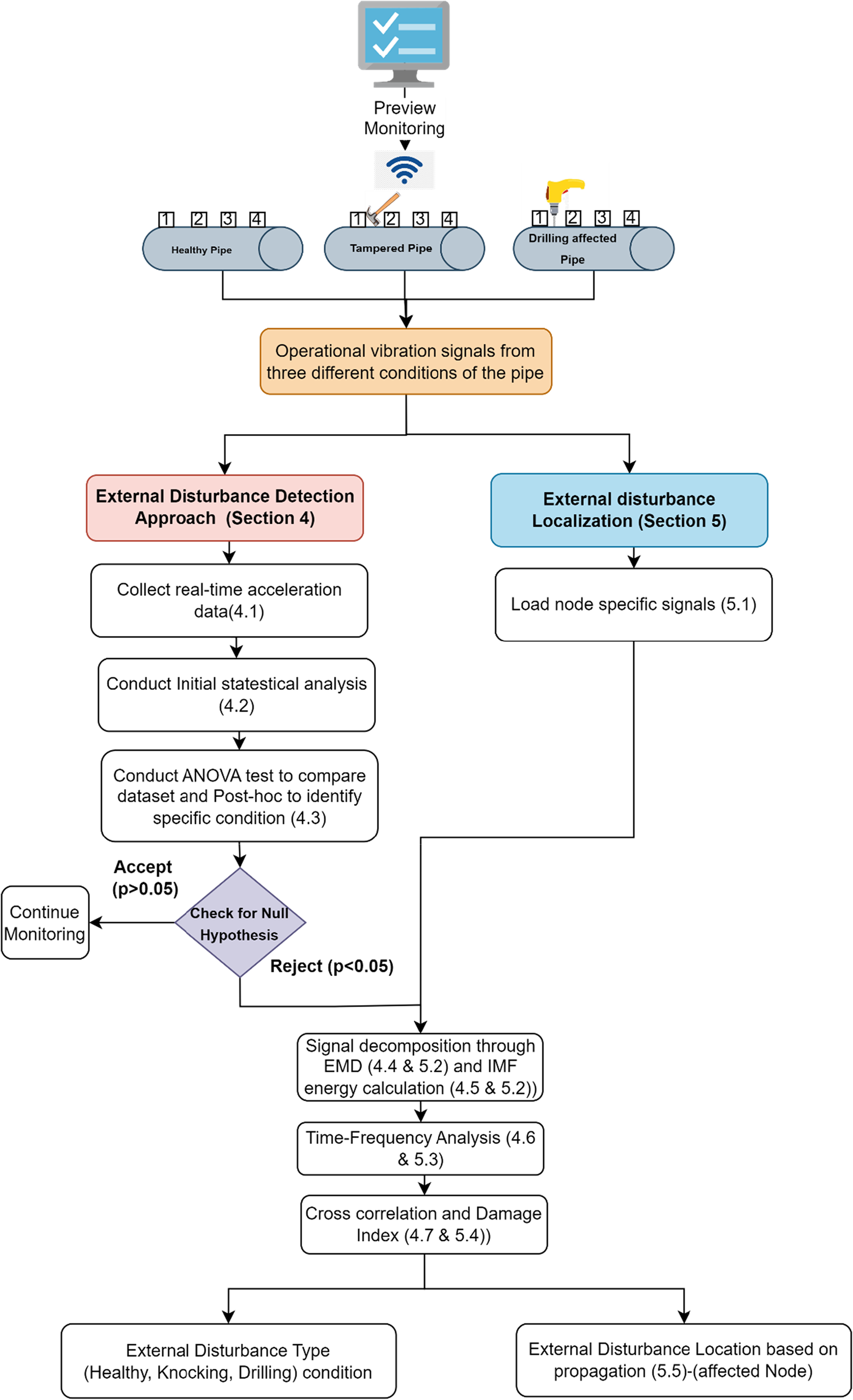

It integrates a series of preprocessing and analytical techniques. The proposed multimodal approach integrates denoising, statistical analysis, decomposition, and advanced techniques, including correlation between different data sources. After validation with experiment data, the system can be trained to process, analyze, and monitor continuous real-time data.

Fault localization begins by loading the node-specific signals and directly proceeding to EMD decomposition, bypassing the initial statistical analysis steps (e.g., histogram, QQ plot, ANOVA, and post-hoc tests) used in external disturbance identification. This streamlined approach is adopted because the external disturbance was identified in the previous stage. By starting directly with EMD decomposition, the focus shifts from identifying the external disturbance to pinpointing its location.

Data-driven multimodal approach for detection of external disturbances in pipelines

Raw accelerometer signals

The accelerometer data were collected from multiple nodes from three distinct pipe conditions and were normalized using Z-score normalization to standardize the amplitude values. This method ensures the data has a mean of zero and a standard deviation of one, making it dimensionless for unbiased signal comparisons. These pre-processed signals improve the accuracy of subsequent analyses and minimize data distortion.

Pipeline surroundings introduce significant noise due to vibrations, operational flow, and environmental exposure. Basic signal comparison can be unreliable if overlapping signals hinder the true information in the signal. Figure 4 shows the pre-processed accelerometer signals collected from three distinct conditions of the pipe. Each condition contributes to the different types of vibrations.

Figure 4.

Raw accelerometer signals collected from three distinct conditions of the pipe.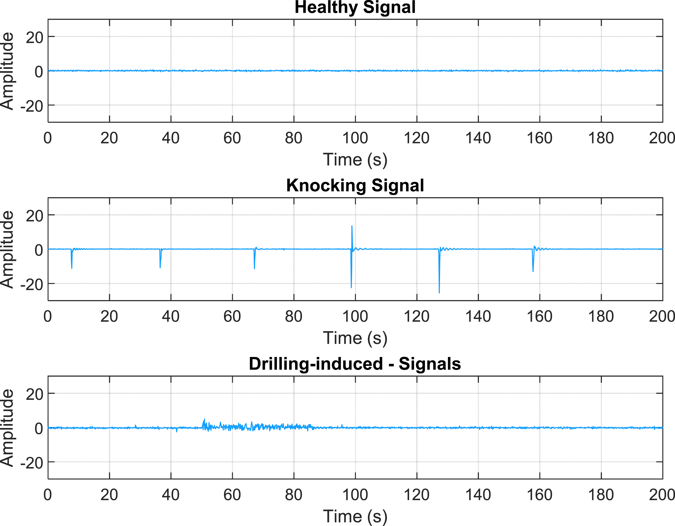

Statistical analysis

Statistical analysis is essential for real-time monitoring and provides quantifiable validation rather than visual comparison. The pre-processed signals are analyzed using statistical tools such as Histogram and QQ plot to observe deviations from normal operational behavior.

Histograms of signals under different conditions visually highlight how the frequency distribution changes with external disturbances, as shown in Figure 5. A QQ plot (equation (5)) compares the sample quantiles of observed data to the theoretical quantiles of a specified distribution. Using the observed mean and standard deviation, the theoretical normal distribution is derived, and its inverse cumulative function calculates the theoretical quantiles. The observed quantiles are then plotted against the theoretical ones, providing a clear visualization of how closely the data aligns with the red line.

QQ plot = \frac{Q_{d a t a}}{Q_{t h e o r y}}

(5)

Figure 5.

Histogram and QQ plot for three distinct conditions of the pipe.

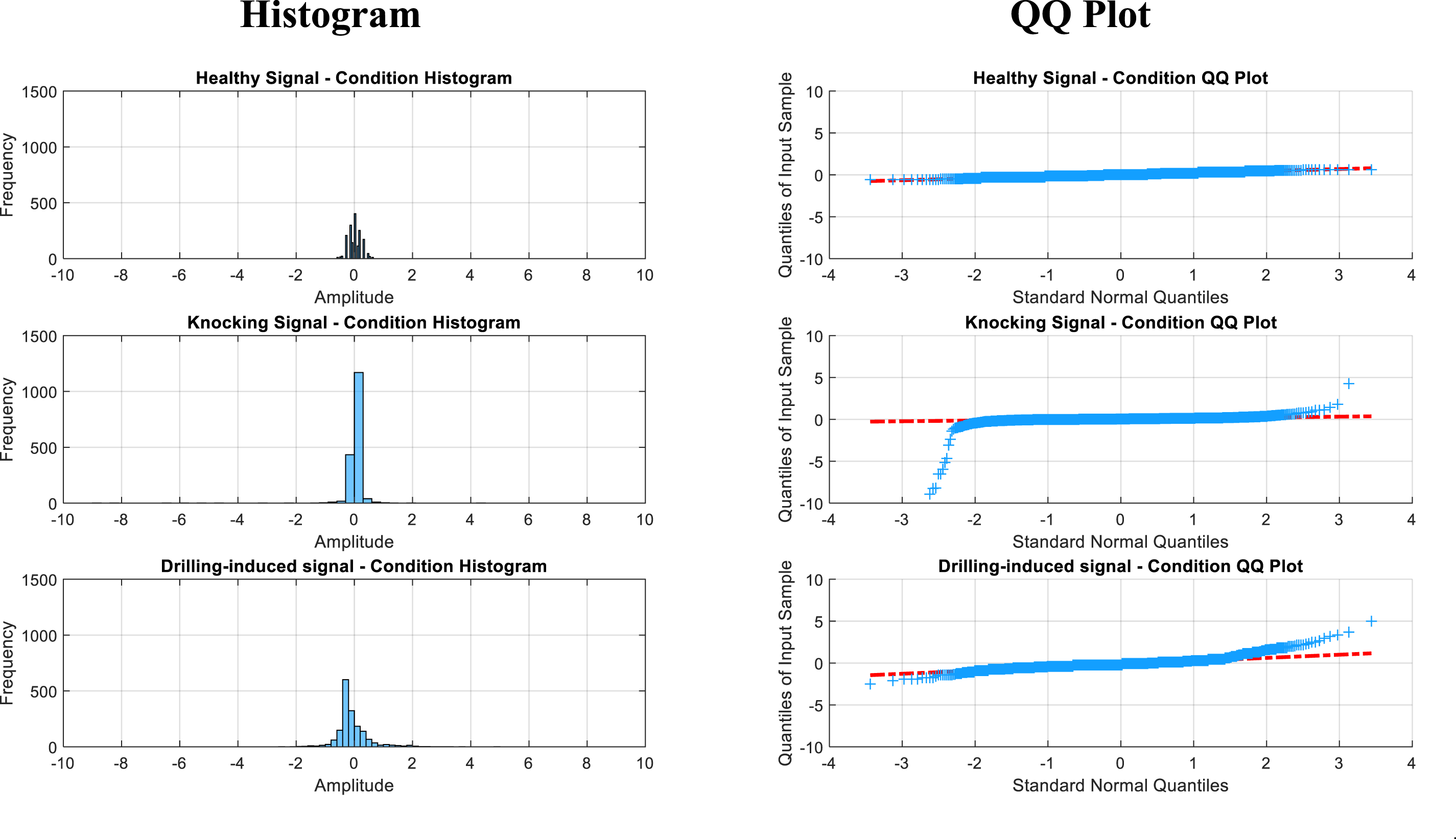
A red line represents the linear regression between the observed quantiles and theoretical quantiles.

The data closely follows the red line in the QQ plot for the healthy pipe, which indicates that the data is approximately normally distributed. However, during disturbance events such as knocking and drilling, the data points deviate significantly from the expected pattern, exhibiting heavy tails that suggest irregularities and departures from normality. For real-time systems, threshold values based on historical data can be set to trigger alerts when statistical outliers are detected.

Statistical estimation through ANOVA test and post-hoc analysis

When deviations are observed, a One-Way ANOVA test is used to assess the significance of variations across datasets. This test determines whether the recorded changes are statistically different or it is just random fluctuations. Post-hoc analysis follows to identify specific conditions showing significant differences. Together, these analyses provide a statistical backbone for validating and distinguishing the disturbances. Together, these analyses validate and distinguish disturbances, forming a statistical foundation for anomaly or intrusion detection.

The calculation involved is outlined in equations (6)–(12).

The mean of each condition of the pipe:

\bar{X_{h}} = \frac{1}{n_{h}} \sum_{j = 1}^{n_{h}} X_{h j}, \bar{X_{k}} = \frac{1}{n_{k}} \sum_{j = 1}^{n_{k}} X_{k j}, \bar{X_{i}} = \frac{1}{n_{d}} \sum_{j = 1}^{n_{d}} X_{d j}

(6)

where X_h, X_k, and X_d represent the individual values for the healthy, knocking, and drilling conditions, respectively.

Overall mean across all conditions:

\bar{X} = \frac{1}{n} (\sum_{j = 1}^{n_{h}} X_{h j} + \sum_{j = 1}^{n_{k}} X_{k j} + \sum_{j = 1}^{n_{i}} X_{d j})

(7)

where

n = n_{h} + n_{k} + n_{d}

The sum of the square between conditions (SSB):

S S B = n_{h} {(\bar{X_{h}} - \bar{X})}^{2} + n_{k} {(\bar{X_{k}} - \bar{X})}^{2} + n_{d} {(\bar{X_{d}} - \bar{X})}^{2}

(8)

The sum of squares within the conditions (SSW):

S S W = (\sum_{j = 1}^{n_{h}} {(\bar{X_{h j}} - \bar{X_{h}})}^{2} + \sum_{j = 1}^{n_{k}} {(\bar{X_{k j}} - {\bar{X}}_{k})}^{2} + \sum_{j = 1}^{n_{i}} {(\bar{X_{d j}} - {\bar{X}}_{d})}^{2})

(9)

Mean square between groups (MSB):

M S B = \frac{S S B}{3 - 1} = \frac{S S B}{2}

(10)

Mean square within the groups (MSW):

M S W = \frac{S S W}{n - 3}

(11)

F_{S t a t i s t i c} = \frac{M S B}{M S W}

(12)

The F-statistic indicates whether the group means differ significantly from one another. The p-value is calculated alongside the F-value for each predictor against the response variable. For a variable to be significant, its p-value must be less than the alpha level (typically defined as 0.05). This threshold is commonly used in pipeline condition analysis to predict and classify failures.⁴⁰ Prior studies have applied ANOVA and the F-test to identify significant features in input datasets. In the model proposed by Arowolo, the p-value^41,42 is used as a measure of statistical significance and rejects the null hypothesis when it falls below 0.05.

As shown in Table 3 (obtained from the ANOVA test corresponding to Figure 6), data for the healthy condition of the pipe shows a narrow range (minimum: −0.57542, maximum: 0.62347), with no outliers. The lower and upper adjacent values (−0.57542 to 0.6234) are closely aligned with the observed range, indicating a steady response without significant variations. This steady behavior confirms normal operating conditions with no external interference.

Table 3.

ANOVA test summary for conditions of the pipe.

Condition	Maximum	Minimum	No. of outliers	Lower adjacent	Upper adjacent	F-Statistics	p-value
Healthy pipe	0.6234	−0.5754	0	−0.57542	0.6234	4.85	0.0078
Tampered pipe	13.651	−25.47	145	−0.15016	0.26805
Drilling-affected pipe	4.994	−2.499	121	−1.1369	0.79346

Figure 6.

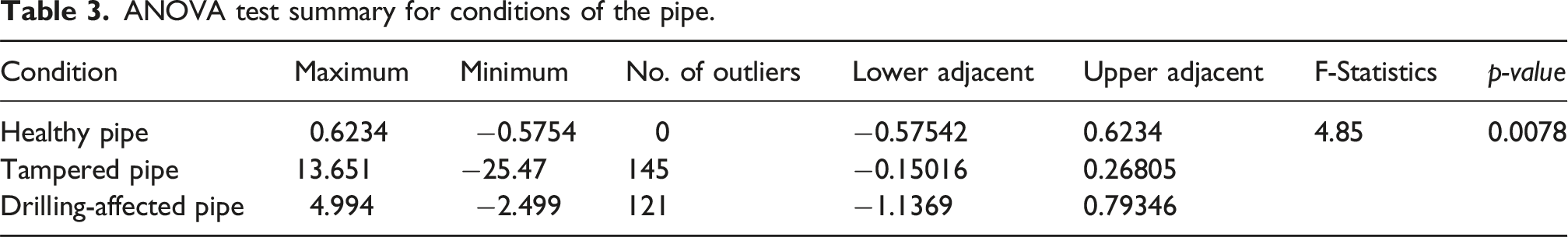
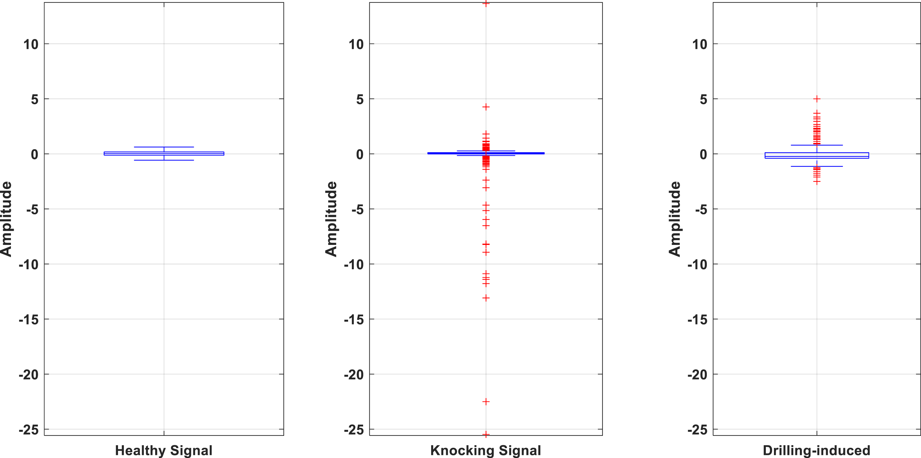
ANOVA test for three different conditions of the pipe.

The knocking condition exhibits a significantly wider range (minimum: −25.475, maximum: 13.651) with 145 outliers detected. However, adjacent values are much closer compared to the data spread. This indicates that most of the data lies in a narrow steady range but is disrupted by extreme fluctuations. The behavior suggests substantial disturbance due to the multiple knocking effect, which generates high-magnitude outliers and irregularity in the data.

The drilling-affected pipe has a moderate range (minimum: −2.4995, maximum: 4.9948) with 121 outliers. The adjacent value (−1.1369 to 0.79346) covers the border range compared to a healthy pipe, signifying prolonged but less intense external interference compared to knocking. The null hypothesis is rejected as the p-value is less than 0.05.

In real-time analysis, large volumes of continuous data make a comprehensive evaluation of every signal impractical. ANOVA provides an efficient screening tool to identify datasets with significant variations and avoid unnecessary analysis of stable conditions. Once significant deviations are detected, post-hoc tests pinpoint the specific conditions responsible.

Post-hoc test compares the mean of each condition to determine if the difference between their means is statistically significant.

The test statistic for the post-hoc test is given in equation (13):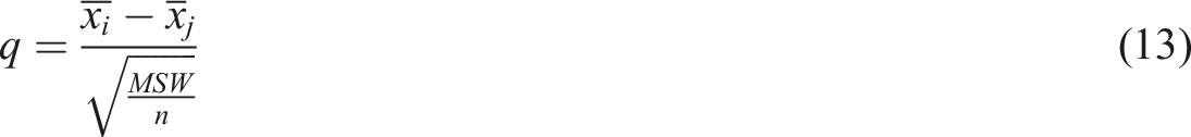

q = \frac{\bar{x_{i}} - {\bar{x}}_{j}}{\sqrt{\frac{M S W}{n}}}

(13)

The post-hoc plot (Figure 7) illustrates the statistical relationships between the pipeline conditions. The plot highlights positive mean differences (bars) for all pairwise comparisons. For healthy versus knocking and knocking versus drilling, the confidence intervals (black error bars) span both negative and positive values. This indicates that the difference between these conditions is not significant. However, both comparisons show positive mean differences. On the other hand, for healthy versus drilling, the confidence interval indicates a statistically significant difference between the conditions. These findings confirm significant deviations and uncertainties between most conditions.

Figure 7.

Post-hoc plot for three distinct pipe conditions.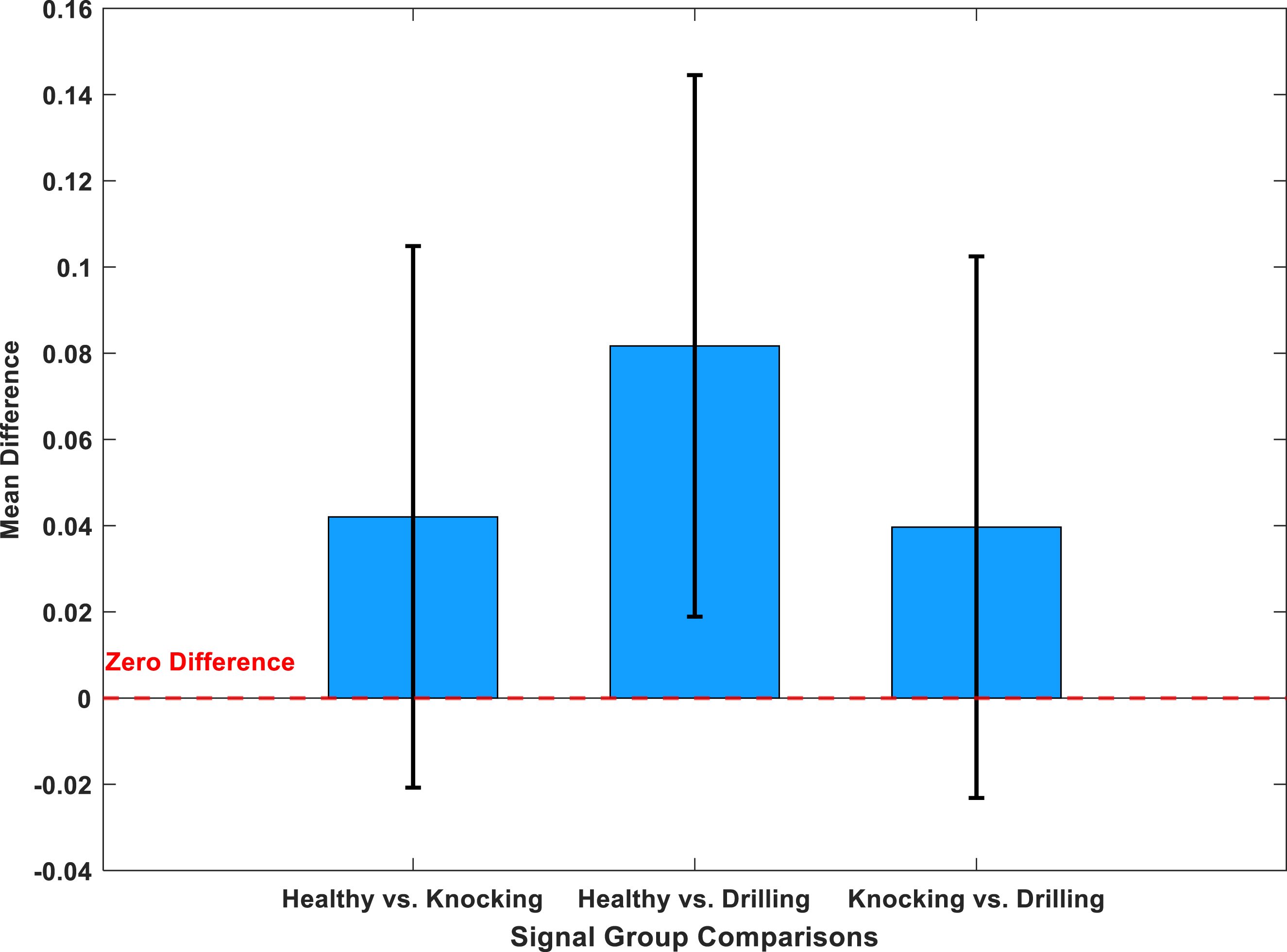

Empirical mode decomposition (EMD)

After verifying condition-specific differences, each condition’s signals were decomposed into IMFs based on inherent oscillatory modes present in the data, which makes it more suitable for transient or irregular data using EMD. The fundamental theory of EMD is systematically outlined to enhance fault characteristic frequency identification⁴³ and its application in analyzing accelerometer responses for structural health monitoring.⁴⁴

As shown in Figure 8, each IMF represents a distinct frequency and amplitude component of the signal. The analysis of IMF provides the isolation of low-frequency fluctuations and high-frequency components. External disturbances in pipelines are exhibited differently. Knocking is characterized by sharp impacts appearing in high-frequency zones with high-amplitude bursts in specific IMFs while drilling produces low-frequency and sustained oscillations that signify continuous disturbances. This separation allows for the extraction of transient features like bursts or sustained fluctuations for further analysis.

Figure 8.

Decomposition of accelerometer signals into the first four intrinsic mode functions (IMFs) for three distinct pipeline conditions.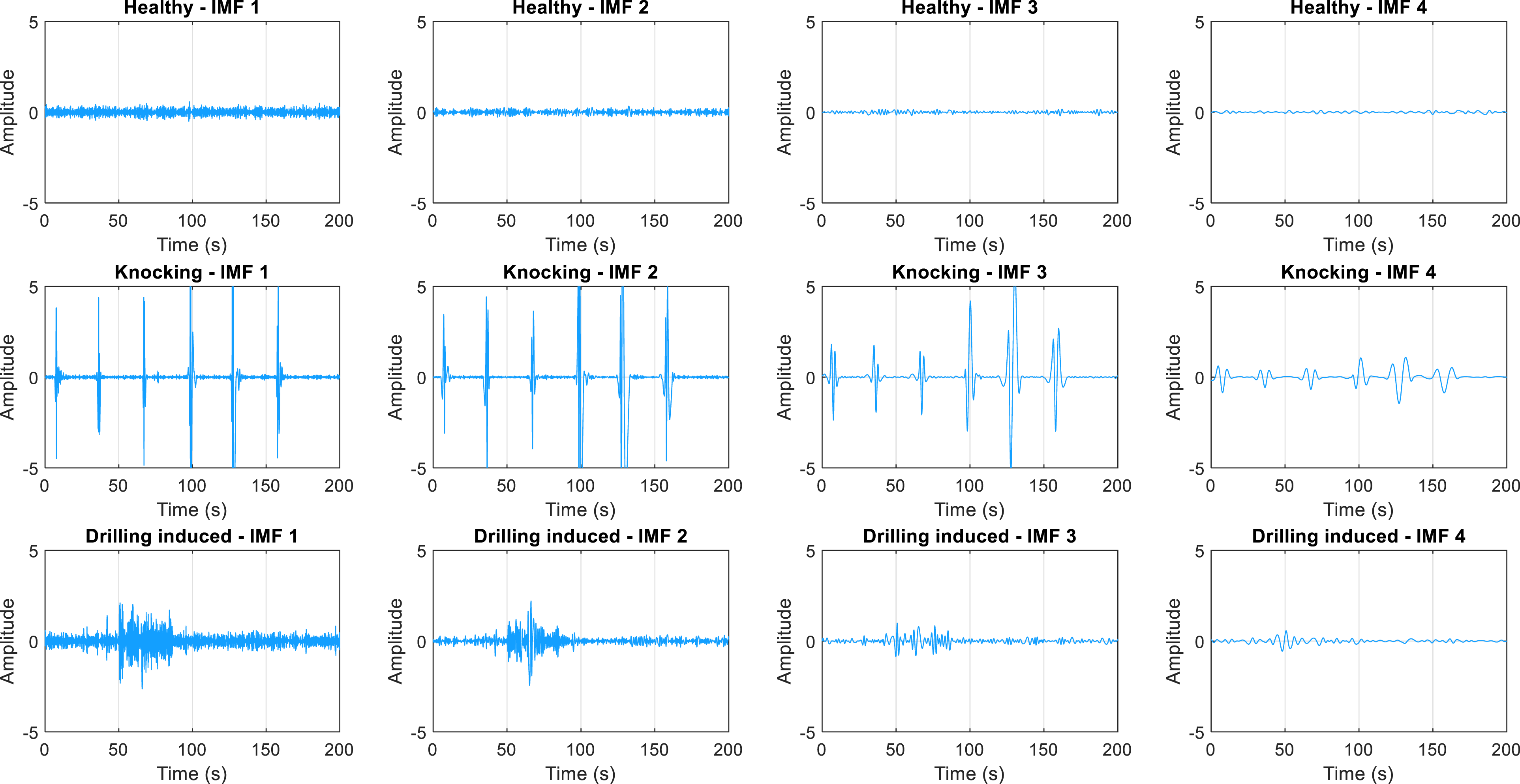

Energy calculation for IMFs for feature selection

As observed in the previous section, mechanical disturbances may generate high-frequency vibrations and low-sustained oscillations. Therefore, it is essential to calculate the energy of IMF signals to assess their strength (equation (14)).

E_{i} = \int_{0}^{T} {| {I M F}_{i} (t) |}^{2} d t

(14)

By calculating the energy of each IMF and selecting those with the higher energy, the most significant component of the signal which may contain valuable information about the external disturbance can be identified.

The energy distribution in IMFs, as shown in Figure 9, effectively distinguishes between pipeline conditions. Knocking results in concentrated energy spikes in high-frequency IMFs, whereas drilling shows energy spread across multiple IMFs. This distinction in energy patterns helps differentiate the type of mechanical disturbances.

Figure 9.

IMFs energy for three distinct conditions of the pipe.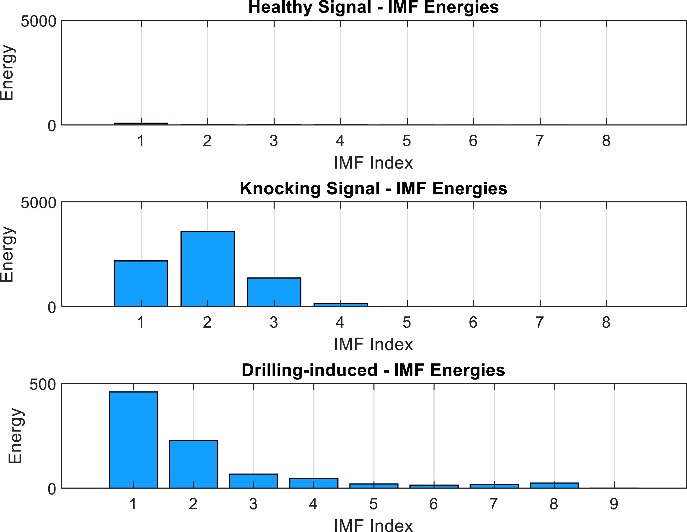

Wavelet analysis

Energy calculation highlights the key vibrational modes and frequency patterns associated with specific disturbances. To visualize these patterns, wavelet analysis is applied to the IMFs with higher energy. This can highlight the specific pattern related to transient or periodic events. Identification of these disturbances is challenging as they do not affect the whole signal, and these events may not affect the entire signal. It is challenging to identify using the traditional Fourier transform, which only provides frequency information without time localization.

In this study, the CWT was performed using the analytic Morlet wavelet (“amor”) to transform the first three IMFs into the time–frequency domain.

The wavelet transforms into an ${I M F}_{i} (t)$ which is given by equation (15):

Continuous wavelet transform (CWT) is used:

W (a, b) = \frac{1}{\sqrt{a}} \int_{- \infty}^{\infty} {I M F}_{i} (t) ψ^{*} (\frac{t - b}{a}) d t

(15)

where

ψ

is the wavelet function, a is the scale parameter, and b is the translation parameter.

Signals with time-varying frequencies are a common characteristic of the faults. By using this wavelet, the system enhances its ability to capture subtle variations and effectively analyze non-stationary signals, such as those generated by external disturbances in pipelines by maintaining a good balance between time and frequency resolution.

Wavelet analysis captures these changes accurately in the time–frequency space and allows clear visualization of transient events. The wavelet coefficients for different disturbances show distinct patterns in the wavelet power spectra. As shown in Figure 10 for the knocking diagram, clear high-frequency bursts represent multiple knocking effects with time events effectively captured, whereas low-frequency vibrations are visible in the drilling-induced disturbance.

Figure 10.

Wavelet analysis of the first three IMFs for three distinct conditions of the pipe.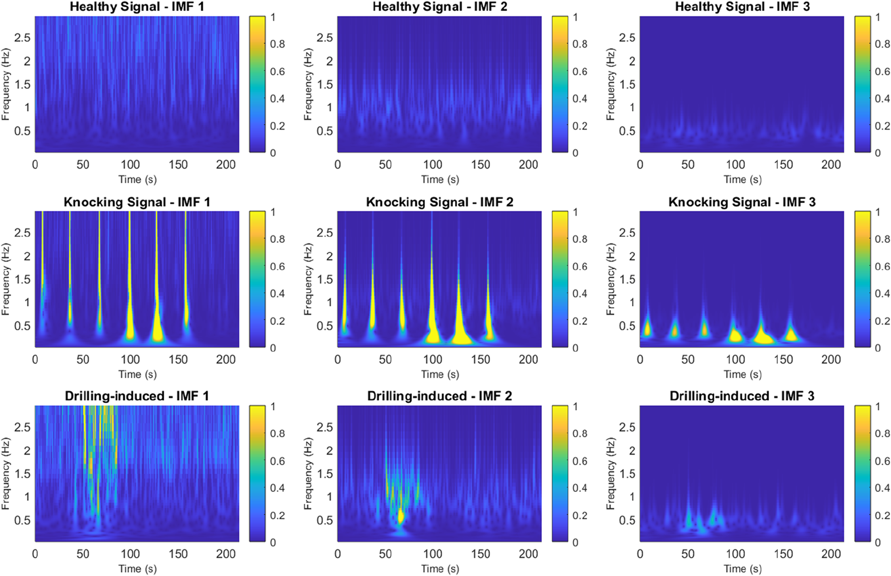

Cross-correlation analysis

The cross-correlation matrix and the damage index matrix provide valuable insights into the relationships between the conditions and their respective disturbances.

The cross-correlation between two wavelet coefficient signals at decomposition level 3 for both the pair of the signal by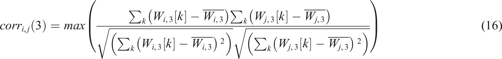

{c o r r}_{i, j} (3) = \max (\frac{\sum_{k} (W_{i, 3} [k] - \bar{W_{i, 3}}) \sum_{k} (W_{j, 3} [k] - \bar{W_{j, 3}})}{\sqrt{({\sum_{k} (W_{i, 3} [k] - \bar{W_{i, 3}})}^{2})} \sqrt{({\sum_{k} (W_{j, 3} [k] - \bar{W_{j, 3}})}^{2})}})

(16)

The damage index can be calculated as

D_{i, j} = 1 - {c o r r}_{i, j} (3)

(17)

The damage index matrix is

D I (i, J) = {D I}_{i, j} + {D I}_{j, i}

(18)

Figure 11 represents the cross-correlation matrix between the two signals. The low cross-correlation value between healthy and knocking signals suggests minimal similarity, as knocking produces distinct and impactful features that are easily distinguishable from the healthy condition. The higher correlation between healthy and drilling signals indicates subtle but noticeable changes. A moderate correlation between knocking conditions and drilling-induced vibration reflects the similarity in terms of external disturbance, but the nature of the disturbance varied, making the difference more noticeable.

Figure 11.

Cross-correlation matrix between (a) healthy signal versus knocking signal, (b) healthy signal versus drilling-induced signal, and (c) knocking signal versus drilling-induced signal.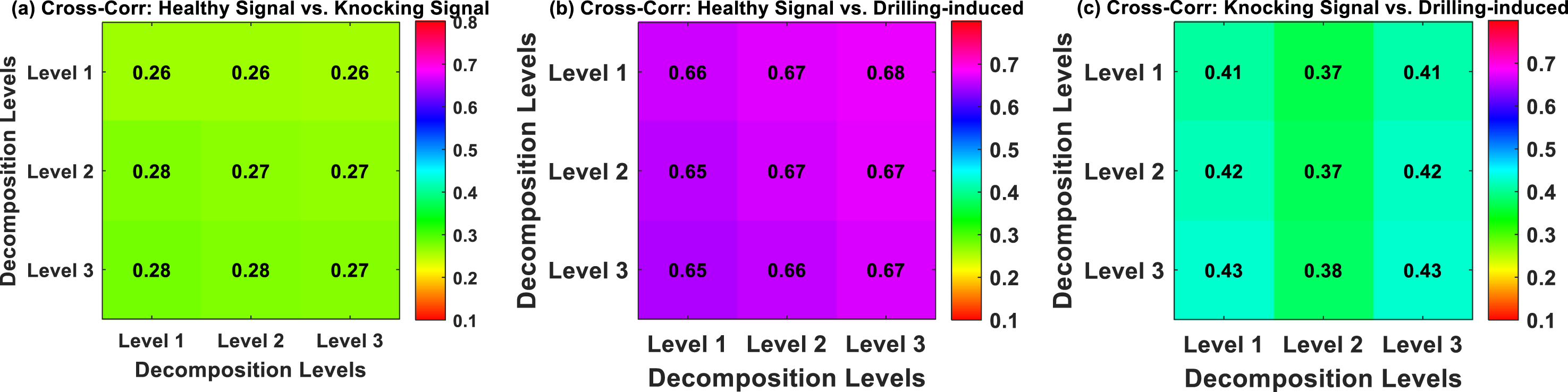

The damage matrix (Figure 12) is calculated to quantify the relative disturbance between condition pairs. The high damage index value (0.7192) for the healthy versus knocking condition reveals that knocking induces impactful disturbance to the pipeline. In contrast, the lower value of 0.3241 for the healthy versus drilling condition indicates a less pronounced disturbance caused by drilling, though still measurable.

Figure 12.

Damage index matrix for three distinct conditions of the pipe.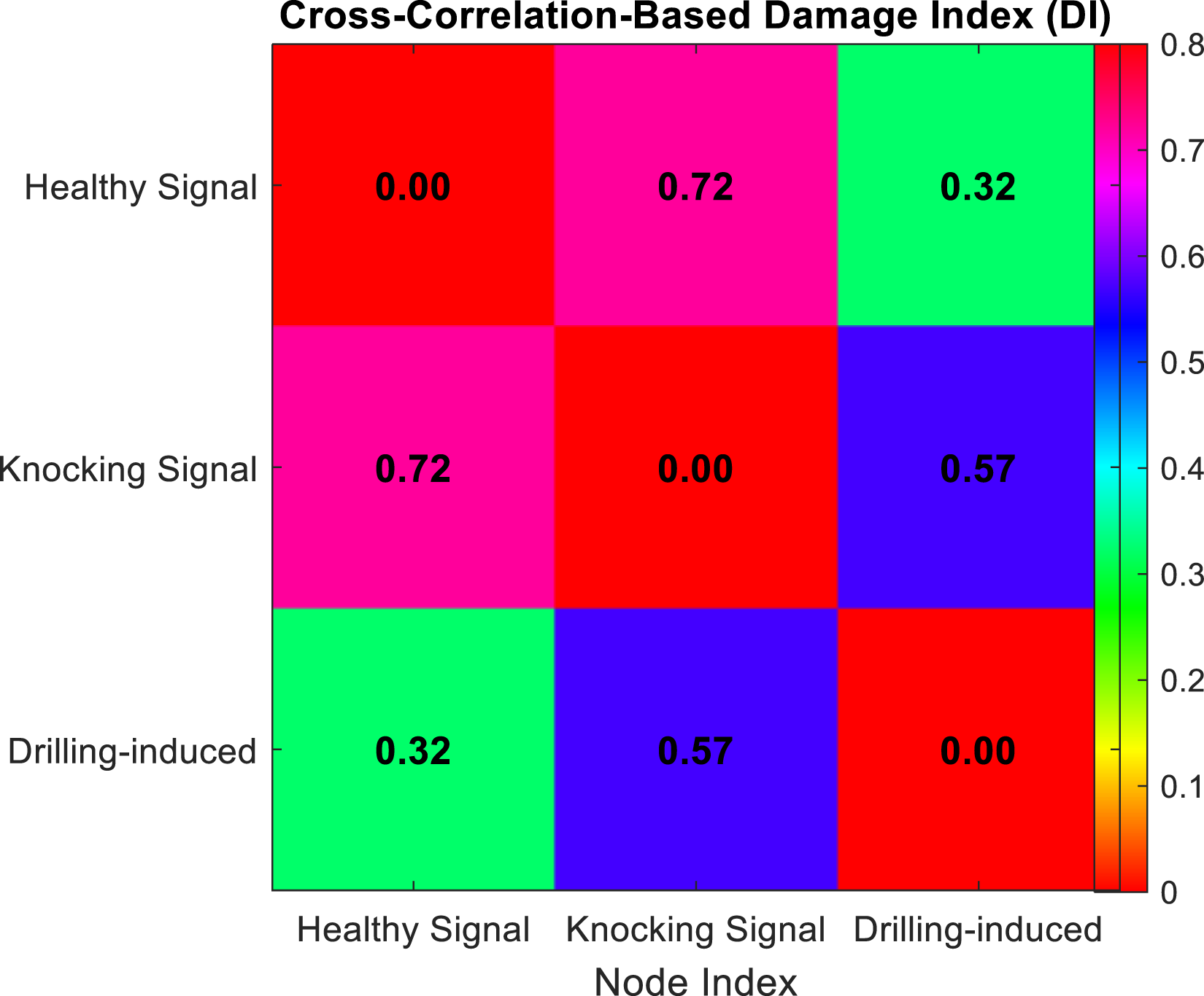

Overall, these analyses confirm that knocking and drilling induce distinct types of disturbances that can be easily identified. This approach provides a framework for the timely detection of external disturbances in pipelines to reduce the risk of damage.

Data-driven multimodal approach for localization of external disturbances in pipelines

Accelerometer data collection from multiple nodes

Accelerometer signals were collected from four nodes mounted on the pipeline, as shown in Figure 2. These signals capture the vibration patterns caused by external disturbances. The collected data is used for the analysis of the localized effects and their propagation along the pipeline. For the knocking simulation, the impact was applied near Node 2, as shown in Figure 13, to observe the disturbance’s influence.

Figure 13.

Time waveforms recorded at each node for the knocking event.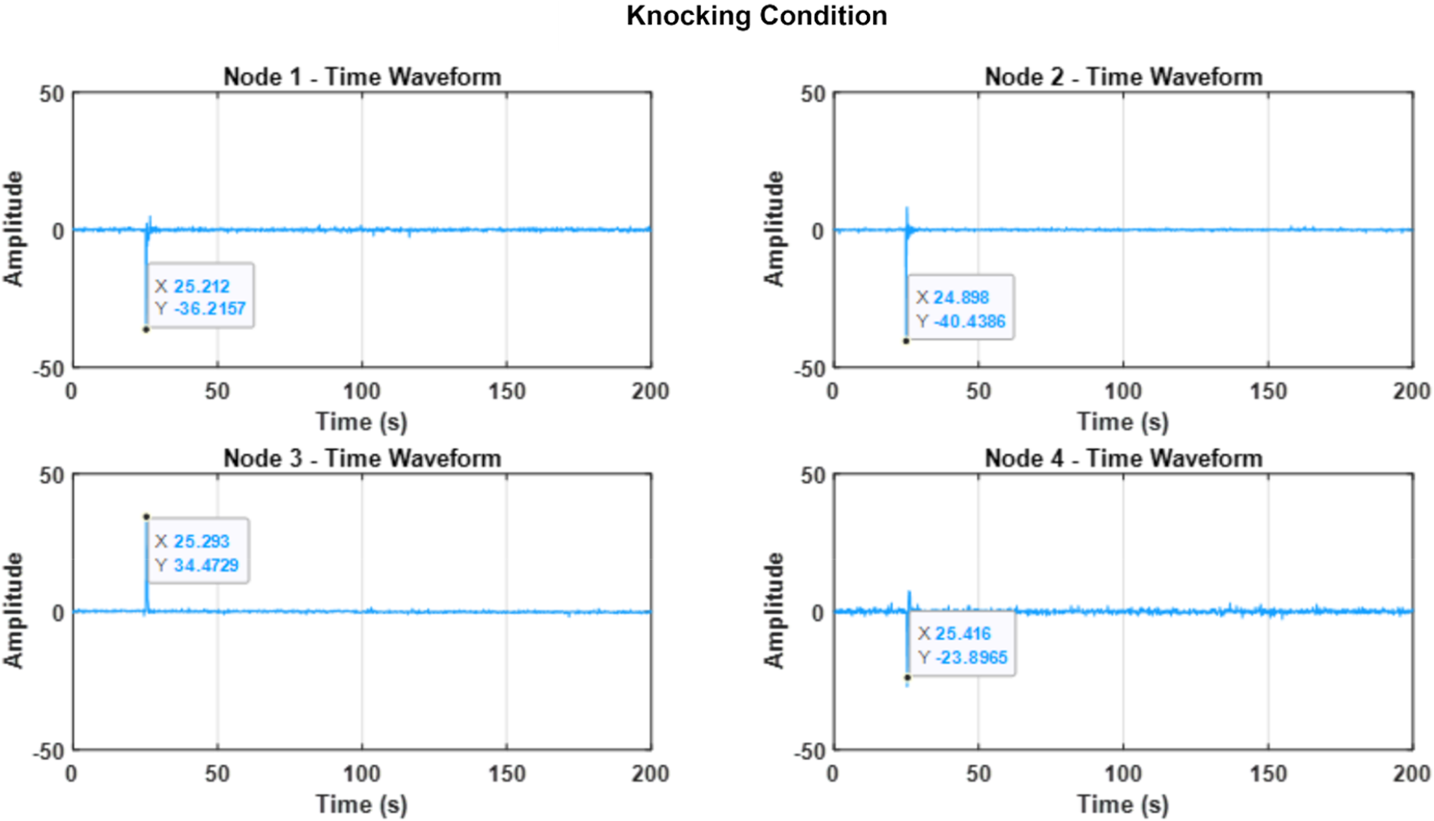

The time waveform data shown in Figure 13 reveals the dynamic response of the pipe to the hammer strike. Each accelerometer recorded variations in the waveform due to the frequency content of the impact and the influence of pipe vibrational modes on wave propagation. Node 2 recorded the earliest and highest amplitude response, while the other nodes experienced a slight delay (milliseconds) and reduced amplitude. These variations in timing and amplitude provide valuable insights into wave propagation characteristics and assist in the effective localization of external impacts. The distance between accelerometers and wave propagation dynamics influences the delayed peak response and amplitude reduction.

Vibration due to drilling is induced near Node 2 for a few seconds and repeated three times as shown in Figure 14. The time waveform data shows similar effects across all nodes.

Figure 14.

Time waveforms recorded at each node for the drilling event.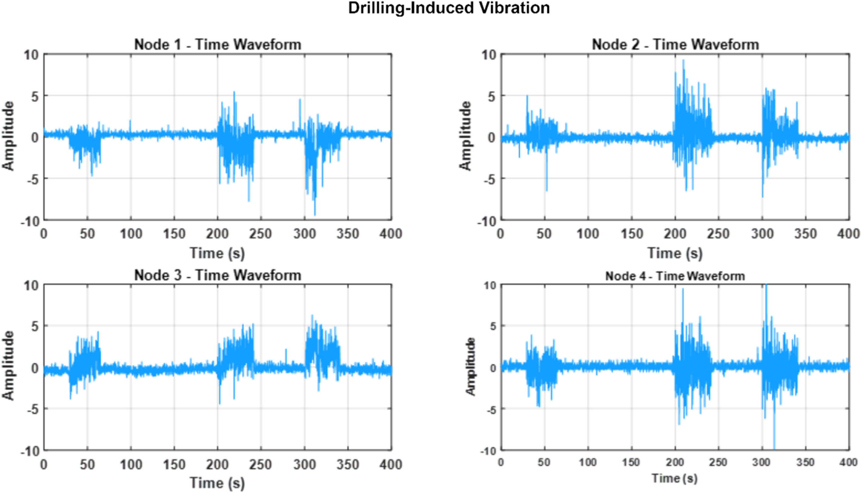

It is challenging to identify the source of the impacted node. Since drilling generates low-frequency vibrations, these vibrations can propagate farther. This results in similar responses being recorded at each node.

Empirical mode decomposition (EMD) and IMFs energy

The signals from each node undergo EMD to extract IMFs. This step highlights dominant vibration modes for each node to identify the affected nodes and the source of disturbance.

The knocking signals recorded from Node 1 to Node 4 undergo EMD to extract the IMFs. EMD was applied to decompose the accelerometer signals of knocking events (Figure 15(a) and drilling-induced (Figure 16(a)) signals across four nodes into IMFs to analyze the energy distribution across different frequency bands. By examining the energy plots for both drilling and knocking events, how the disturbances affect different nodes can be observed. This supports the differentiation between high-frequency, localized impacts (knocking) and low-frequency, more widespread effects (drilling).

Figure 15.

(a) EMD decomposition of the knocking signal from four nodes, showing the intrinsic mode functions (IMFs) derived from the accelerometer data, and (b) IMF energy plot for each node.

Figure 16.

(a) EMD decomposition of the drilling-induced signal from four nodes, showing the intrinsic mode functions (IMFs) derived from the accelerometer data, and (b) IMF energy plot for each node.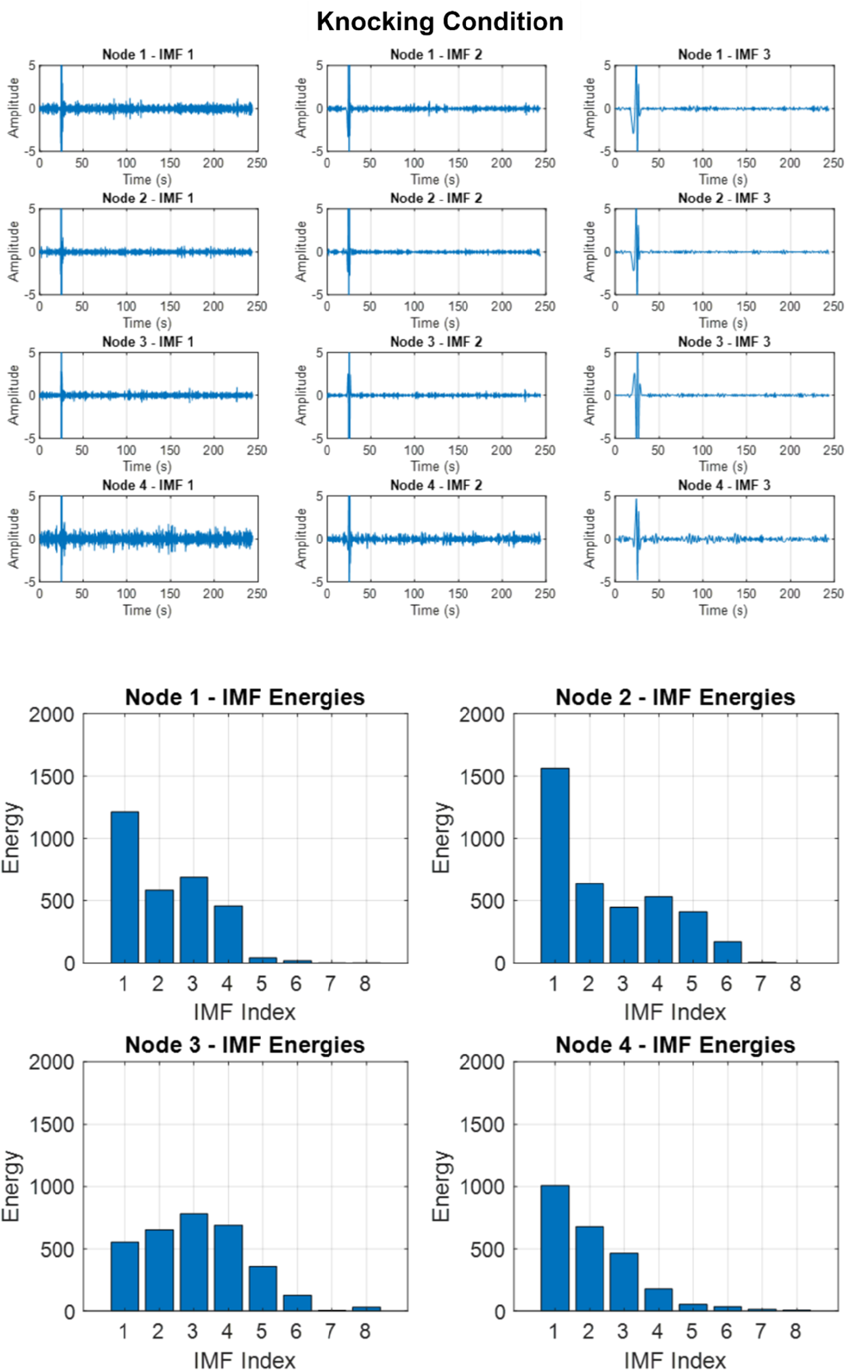

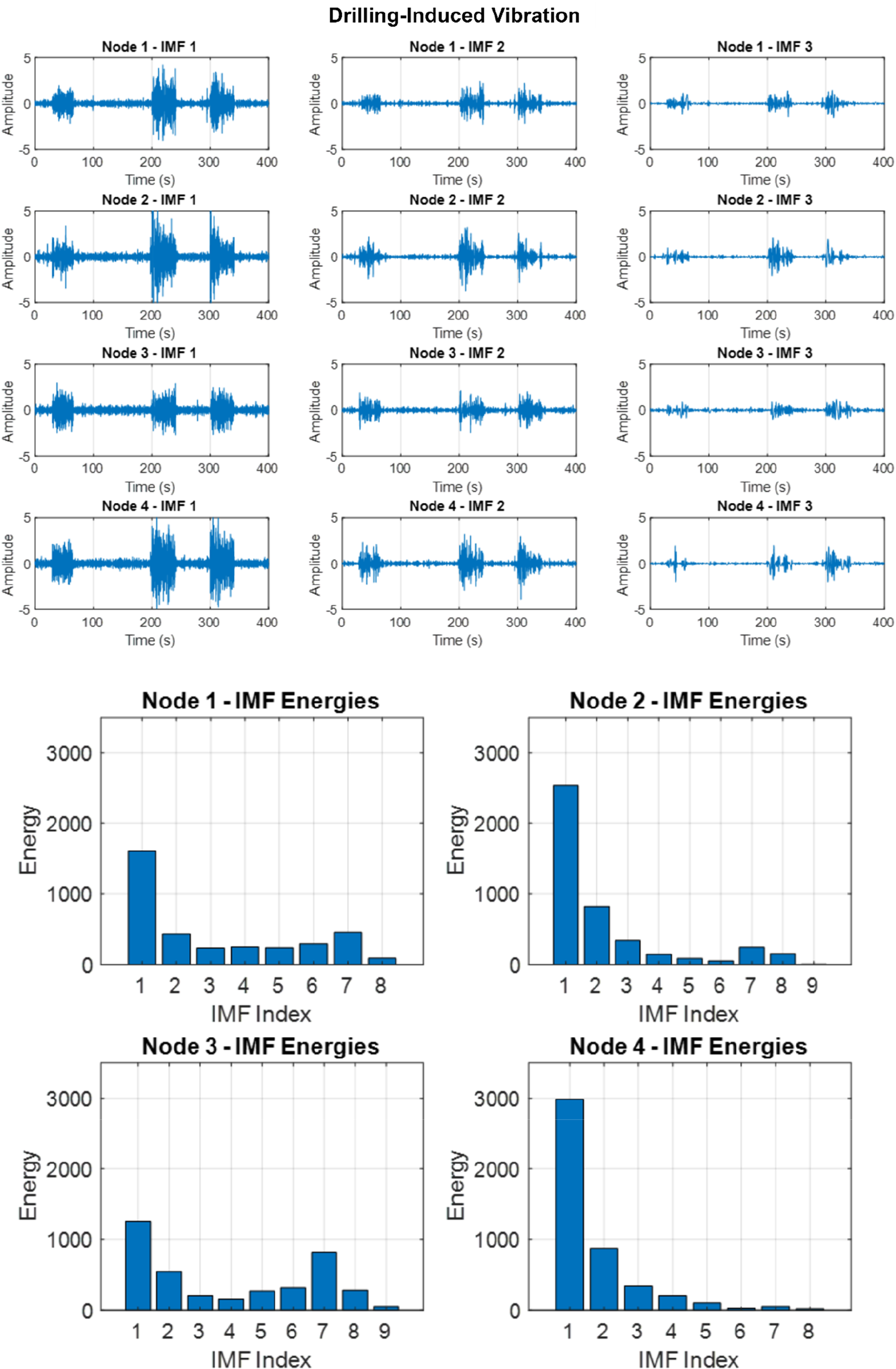
The energy distribution of the IMFs for the knocking event (Figure 15(b)) reveals that knocking generates high-frequency spikes, with the highest energy observed in the first IMF for all nodes (with Node 2 having the highest), except for Node 3. The impact generates a broad range of frequencies across all nodes, but the magnitudes vary, which is a useful indicator for external disturbance localization. Energy for IMF 2 remains nearly similar across the nodes, while Node 3 and Node 4 capture energy across a wider range of IMFs, extending up to IMF 8. This provides valuable insights into the extent of the impact and potential external disturbance localization.

Figure 16(b) shows distinct patterns across the nodes, with Node 1 and Node 4 exhibiting the highest energy in IMF 1, gradually decreasing across higher IMFs. The broad energy spread, particularly at higher IMFs, suggests that drilling generates low-frequency vibrations propagating across the pipeline. However, due to the widespread impact across multiple IMFs and nodes, it becomes challenging to identify the affected node. It allows the identification of distinct disturbance patterns by analyzing the energy distribution across the IMFs, helping to differentiate the nature and spread of the disturbance across the nodes.

Wavelet analysis for time–frequency representation

The wavelet transform provides a visual representation of the disturbance by analyzing the wave’s time–frequency characteristics. The IMFs from each node containing the significant information are processed through wavelet analysis for time–frequency maps. These maps visualize how vibrational energy propagates over time and frequency across the nodes.

The CWT power spectrum analysis for knocking events (Figure 17) reveals that high-frequency waves generated by the impact create a strong amplitude near Node 2, which diminishes rapidly and generates a spike with lower time spread when recorded at Node 1 and Node 3. In contrast, lower frequencies propagate farther with less attenuation when received at Node 4.

Figure 17.

Wavelet analysis of the first three IMFs for each node for the knocking condition.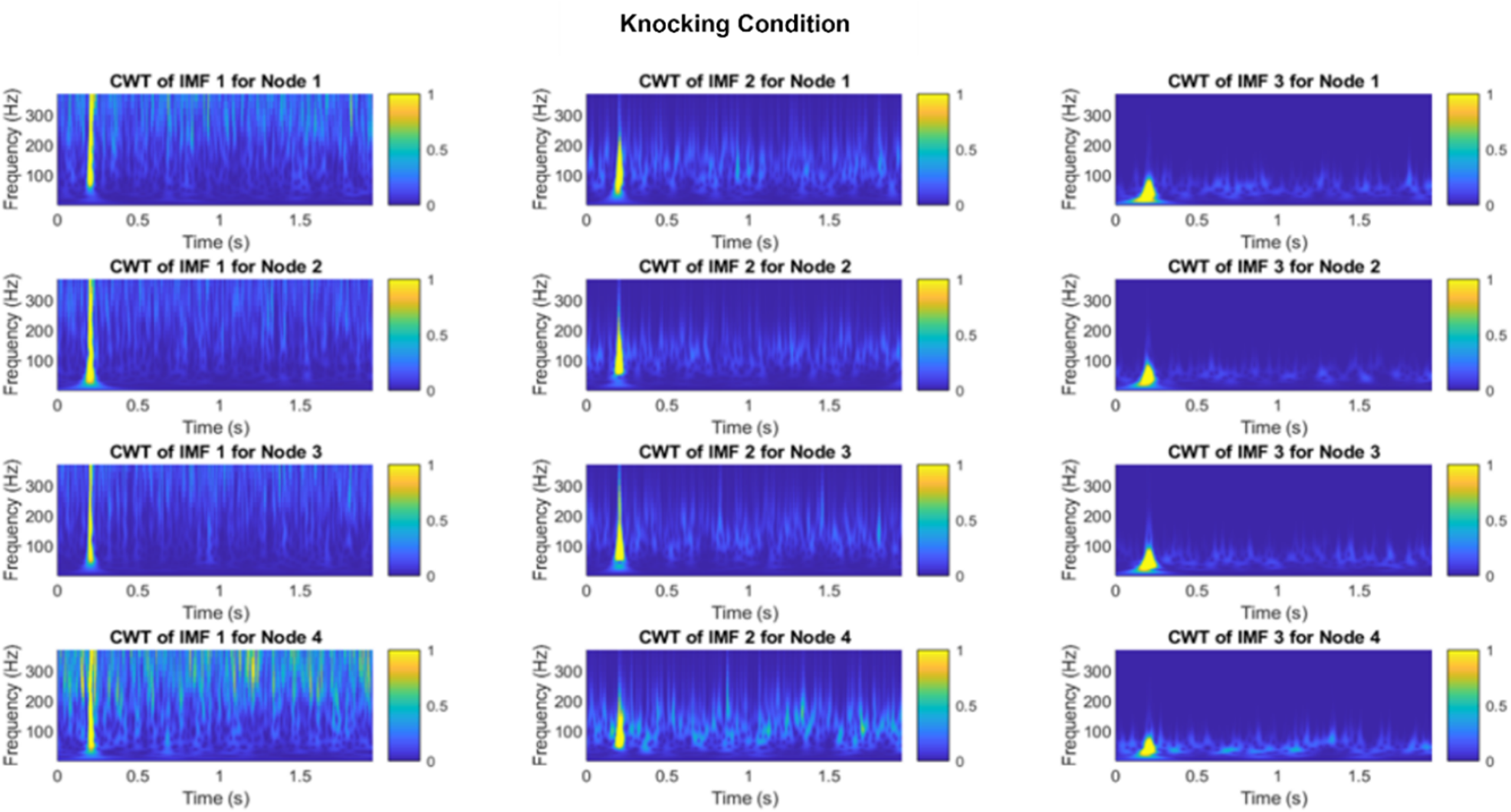

The CWT power spectrum analysis of drilling events (Figure 18) reveals distinct energy propagation across the nodes. Drilling generates low-frequency vibrations, resulting in a broader temporal response at all nodes. Wavelet analysis of IMF 1 shows similar effects at Node 2 and Node 4, while wavelet analysis of IMFs 2 and 3 exhibits higher intensity at Node 2. Though the difference is subtle, this uniform energy distribution across the pipeline makes it challenging to distinguish the drilling source based solely on time–frequency patterns.

Figure 18.

Wavelet analysis of the first three IMFs for each node for the drilling condition.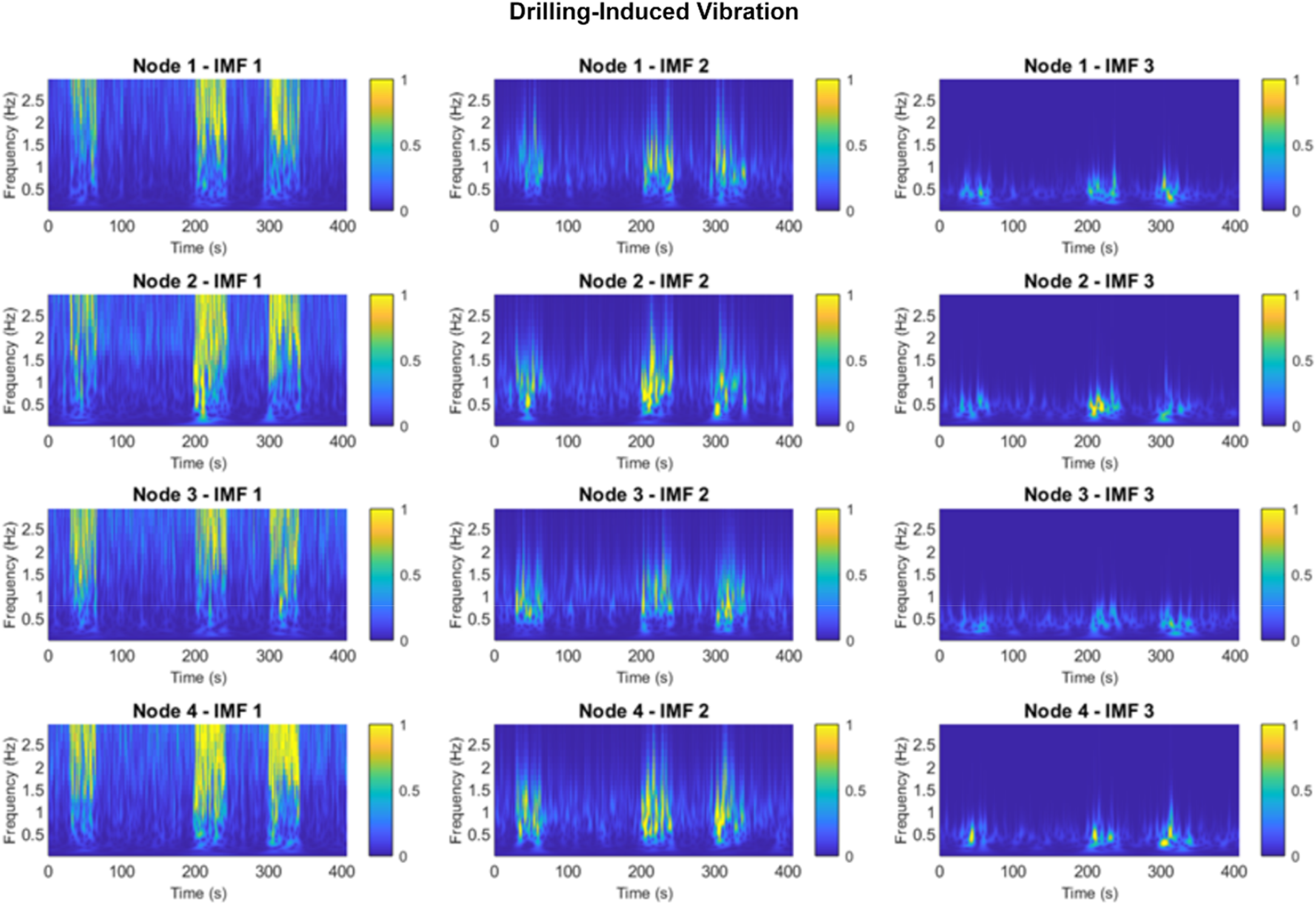

Cross-correlation analysis between nodes

Cross-correlation analysis is performed between the signals from different nodes. This step highlights the propagation of vibrations and the affected zone. The quantitative aspect is needed to assess wave propagation and node-specific impacts. Cross-correlation matrices present numerical values that quantify the coherence and relationship between nodes.

As shown in Figure 19, high correlation values between Node 1 and Node 2 and between Node 2 and Node 3 show strong wave coherence due to their vicinity to the impact site. Similarly, the correlation between Node 1 and Node 3 suggests efficient wave propagation within the nearby nodes. There is a moderate correlation between Node 1 and Node 4, as they are located near the support where wave interaction is influenced by boundary conditions. The weaker correlation highlights that the wave energy reduces as it travels farther from the impact site.

Figure 19.

Cross-correlation matrix between the pair of nodes for knocking condition.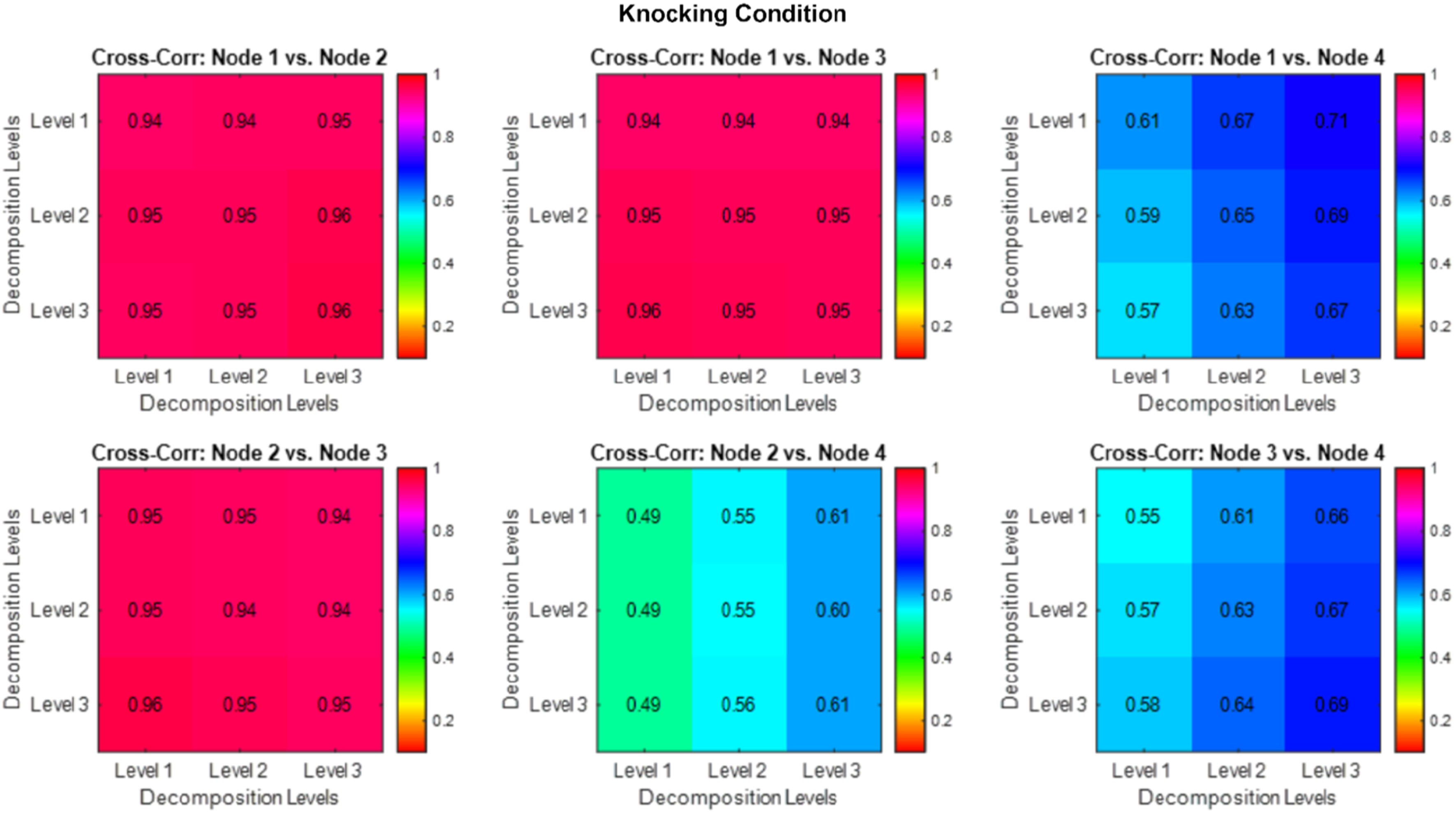

The cross-correlation matrix for the drilling event, as represented in Figure 20, shows similar values across all nodes. This indicates consistent wave propagation and response across the nodes. This uniformity suggests that the low-frequency vibrations generated by the drilling event travel relatively evenly along the pipeline and affect all nodes with similar intensity.

Figure 20.

Cross-correlation matrix between the pair of nodes for drilling-induced vibrations.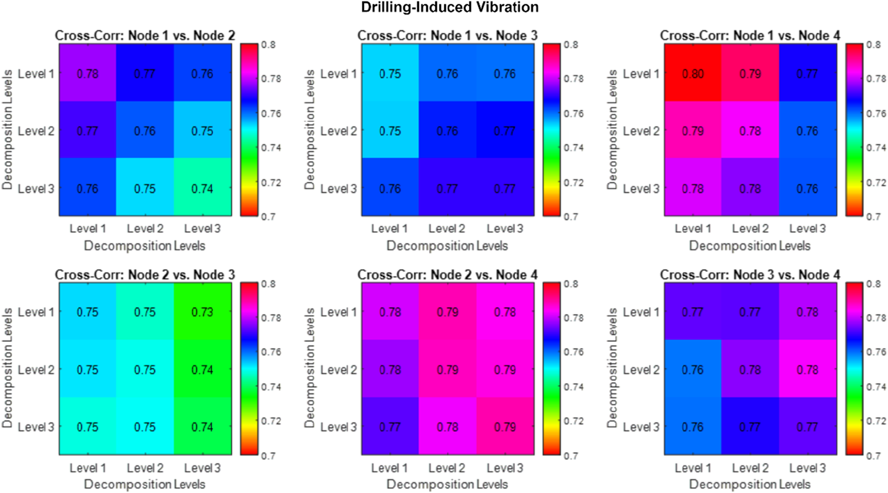

The damage index (DI) can be calculated for each node to quantify the extent of the external disturbance’s influence. The matrix represents the values between different pairs of nodes, which are computed based on their cross-correlation. The diagonal shows zero for the self-comparison. Nodes with higher indices are closer to the external disturbance’s location.

As shown in Figure 21(a), the highest DI values (Node 2 vs Node 4: 0.3941) confirm that the external disturbance or impact site is closest to Node 2. It is consistent with the knocking event being initiated near this node. The damage index matrix for the drilling event (Figure 21(b) reveals a relatively uniform distribution of damage indices across all nodes, with values ranging from 0.2 to 0.2473. The highest values (Node 2 vs Node 3: 0.2473 and Node 1 vs Node 3: 0.2298) suggest coherence between these nodes. Unlike knocking, where damage indices were more concentrated near the impact site, the drilling event generated low-frequency vibrations that propagated uniformly across the pipeline. This uniform distribution reflects the nature of low-frequency waves, which experience less attenuation and dispersion and travel longer distances.

Figure 21.

Damage index matrix (a) for knocking condition and (b) for drilling-induced vibrations.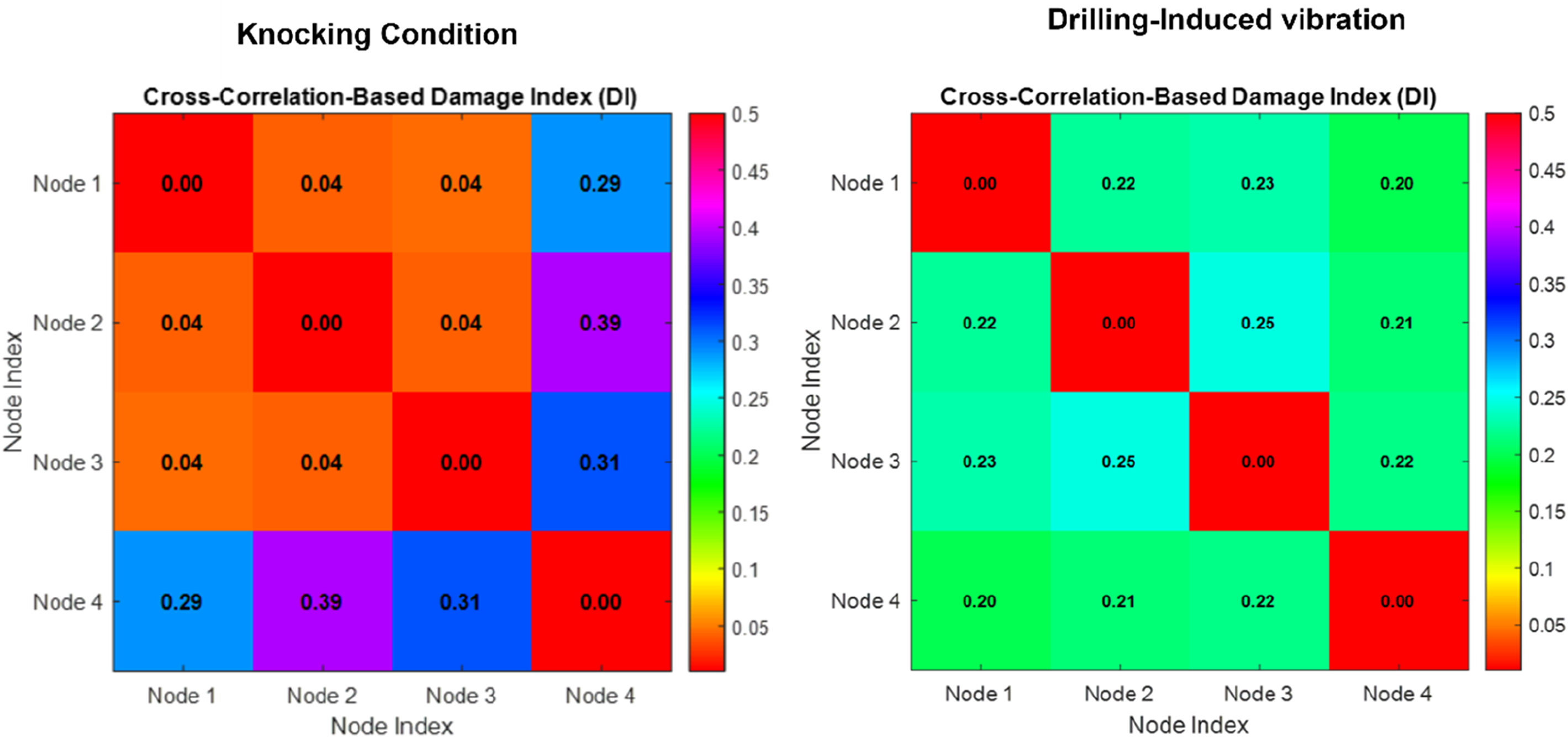

The closely spaced nodes in the current 2-meter pipeline setup further contributed to the uniform detection of drilling vibrations, making pinpointing the exact disturbance location challenging. The dynamics of external disturbance propagation along the pipeline are studied by analyzing time delays and wave propagation patterns from cross-correlation and wavelet results. This includes identifying how quickly the disturbance spreads and its effect on pipeline integrity at various nodes.

Conclusion

The proposed approach effectively addresses external disturbance identification in pipelines. The calculated damage index highlights significant distinctions between different types of disturbances. Knocking induces substantial and easily identifiable disturbances in the pipelines, while the healthy versus drilling condition reflects less pronounced but still measurable disturbances caused by drilling. The findings confirm that knocking and drilling generate distinct disturbance patterns for effectively identifying external damage types.

The external disturbance localization analysis for knocking and drilling events highlights distinct behaviors in wave propagation and their detectability across nodes. Knocking is characterized by its short-lived, high-frequency components, effectively localized near Node 2. This was supported by the sharp amplitude peaks observed at Node 2 and the time lag of signal arrivals at other nodes. The higher damage indices and cross-correlation values between nearby nodes further confirmed the localized nature of the knocking event. In contrast, drilling generated low-frequency vibrations propagating farther due to their longer wavelengths and reduced energy loss. This resulted in a broader time response across all nodes. The low-frequency drilling vibrations were detected uniformly at all nodes in the 2-meter length short pipe and closely spaced nodes in the current setup. This made precise external disturbance localization challenging. However, this behavior provides critical insights into the spatial arrangement of sensors. It emphasizes the importance of optimal node spacing for effective localization of low-frequency disturbances in larger pipeline systems.

Overall, the analysis demonstrates how frequency content influences wave propagation and the localization of external disturbances. Knocking is easier to identify due to its high-frequency nature, while drilling condition highlights the need for improved sensor placement strategies to detect low-frequency events more effectively.

Footnotes

Acknowledgment

This work is supported by Qatar University - International Research Collaboration Grant No. IRCC-2024-002. Open Access funding provided by the Qatar National Library.

ORCID iD

Bhumiben Ankit Shah

Funding

The authors disclosed receipt of the following financial support for the research, authorship, and/or publication of this article: This work is supported by Qatar University—International Research Collaboration Grant No. IRCC-2024-002.

Declaration of conflicting interests

The authors declared no potential conflicts of interest with respect to the research, authorship, and/or publication of this article.

Appendix

References

Shabarchin

Tesfamariam

. Internal corrosion hazard assessment of oil & gas pipelines using Bayesian belief network model. J Loss Prev Process Ind 2016; 40: 479–495.

Wang

Shen

Wang

, et al. Failure probability analysis of the urban buried gas pipelines using Bayesian networks. Process Saf Environ Prot 2017; 111: 678–686.

Iseley

, et al. Pipeline inspection and health monitoring technology: the key to integrity management [Internet]. Springer Nature Singapore, 2023. [cited 2024 Jun 2]. Available from. https://link.springer.com/10.1007/978-981-19-6798-6

Adewumi

Agbasi

Etuk

, et al. An industry perception and assessment of oil and gas pipeline third-party interference. J Int Environ Appl Sci 2023; 18(1): 17–32.

Jaffrey

Lubbers

King

, et al. An effective and proven technique for continuous detection and location of third party interference along pipelines. 2002, 947–952.

. Cause and prevention of pipeline third-party interference. J Natural Gas Industry 2005; 25(12): 118–120.

Mohammed

Ahmed

. Effects of crude oil vandalism on crude oil terminals in Nigeria: 1999–2020. In: Identity, Social Inclusion and Sustainable Development in Nigeria; 2024. p. 669.

Ringbom

Lott

. Sabotage of critical offshore infrastructure: a case study of the balticconnector incident. In: Maritime Security Law in Hybrid Warfare. Brill Nijhoff, 2024, pp. 155–194.

Sanderson

Czub

Koschinski

, et al. Environmental impact of sabotage of the Nord Stream pipelines. 2023.

10.

smartadmin . How armed gangs steal fuel worth millions from buried transnet pipelines - SmartMix technologies, 2022. [cited 2025 Feb 5]. Available from. https://smartmixtechnologie.co.za/how-armed-gangs-steal-fuel-worth-millions-from-buried-transnet-pipelines/

11.

Stanwick

. The environmental challenges of Pemex. International Journal of Management Studies and Social Science Research. 2023; 5: 10–15.

12.

Okoli

Orinya

. Oil pipeline vandalism and Nigeria’s national security. Global J Hum Soc Sci 2013; 13(5): 67–75.

13.

Aroh

Ubong

Eze

, et al. Oil spill incidents and pipeline vandalization in Nigeria: impact on public health and negation to attainment of millennium development goal: the Ishiagu example. Disaster prevention and management. An international Journal 2010; 19(1): 70–87.

14.

Doshmanziari

Khaloozadeh

Nikoofard

. Gas pipeline leakage detection based on sensor fusion under model-based fault detection framework. J Petrol Sci Eng 2020; 184: 106581.

15.

Tian

. A fault detection algorithm for pipeline insulation layer based on immune neural network. Int J Pres Ves Pip 2022; 196: 104611.

16.

Sun

Wang

Duan

. Multiple-fault detection in water pipelines using transient-based time-frequency analysis. J Hydroinform 2016; 18(6): 975–989.

17.

Hussein

Rahim

SBA

Mustapha

, et al. Data-driven multi-fault detection in pipelines utilizing frequency response function and artificial neural networks. J Pipeline Sci Eng 2024; 5: 100223.

18.

Karney

. An overview of transient fault detection techniques. Modeling and monitoring of pipelines and networks: Advanced tools for automatic monitoring and supervision of pipelines. 2017, 13–37.

19.

Quy

Kim

. Crack detection and localization in a fluid pipeline based on acoustic emission signals. Mech Syst Signal Process 2021; 150: 107254.

20.

Lah

Dziyauddin

Yusoff

. Localization techniques for water pipeline leakages: A review. In: 2018 2nd International Conference on Telematics and Future Generation Networks (TAFGEN); 2018. p. 49–54. IEEE.

21.

Pahlavanzadeh

Khaloozadeh

Forouzanfar

. Oil pipeline multiple leakage detection and localization based on sensor fusion. Eng Fail Anal 2025; 167: 109038.

22.

Pérez-Zuñiga

Sotomayor-Moriano

Rivas-Perez

, et al. Distributed fault detection and isolation approach for oil pipelines. Appl Sci 2021; 11(24): 11993.

23.

Galvagni

. Pipeline health monitoring. 2013.

24.

Gong

, et al. An improved method for pipeline leakage localization with a single sensor based on modal acoustic emission and empirical mode decomposition with Hilbert transform. IEEE Sens J 2020; 20(10): 5480–5491.

25.

Wang

Zhu

Wang

, et al. Structural health monitoring of oil and gas pipelines: developments, applications and future directions. Ocean Eng 2024; 308: 118293.

26.

Sharma

Tewari

Biswas

, et al. A comprehensive study of techniques utilized for structural health monitoring of oil and gas pipelines. Struct Health Monit 2024; 23(3): 1816–1841.

27.

Adegboye

Fung

Karnik

. Recent advances in pipeline monitoring and oil leakage detection technologies: principles and approaches. Sensors (Peterb, NH) 2019; 19(11): 2548.

28.

El-Borgi

Patil

, et al. Inspection and monitoring systems subsea pipelines: a review paper. Struct Health Monit 2020; 19(2): 606–645.

29.

Korlapati

NVS

Khan

Noor

, et al. Review and analysis of pipeline leak detection methods. J Pipeline Sci Eng 2022; 2(4): 100074.

30.

Ahmed

Le Mouël

Stouls

, et al. Development and analysis of a distributed leak detection and localisation system for crude oil pipelines. Sensors (Peterb, NH) 2023; 23(9): 4298.

31.

Huang

. Oil and gas pipeline robot localization techniques: a review. Proc IME C J Mech Eng Sci 2024; 238(23): 11049–11067.

32.

Baroudi

Al-Roubaiey

Devendiran

. Pipeline leak detection systems and data fusion: a survey. IEEE Access 2019; 7: 97426–97439.

33.

Gosain

Aggarwal

. IoT based gas pipeline monitoring system. In: 2024 4th International Conference on Technological Advancements in Computational Sciences (ICTACS); 2024. p. 469–476. IEEE.

34.

Ahn

Kim

Choi

. Artificial intelligence-based machine learning considering flow and temperature of the pipeline for leak early detection using acoustic emission. Eng Fract Mech 2019; 210: 381–392.

35.

Zhou

Lin

, et al. Leakage diagnosis and localization of the gas extraction pipeline based on SA-PSO BP neural network. Reliab Eng Syst Saf 2023; 232: 109051.

36.

Rezaei

Taheri

. Health monitoring of pipeline girth weld using empirical mode decomposition. Smart Mater Struct 2010; 19(5): 055016.

37.

Liu

Fang

, et al. Adaptive leak signal extraction based on EMD-CC for water pipeline leak location. Elsevier, 2023, p. 104884.

38.

Xiao

Mao

Tian

, et al. Partial‐model‐based damage identification of long‐span steel truss bridge based on stiffness separation method. Struct Control Health Monit 2024; 2024(1): 5530300.

39.

Xiao

Sun

Mao

, et al. Damage identification of large-scale space truss structures based on stiffness separation method. Elsevier, 2023, pp. 109–118.

40.

Manan

Kamal

Ratlamwala

TAH

, et al. Failure classification in natural gas pipe-lines using artificial intelligence: a case study. Energy Rep 2021; 7: 7640–7647.

41.

Omer Fadl Elssied

Ibrahim

Hamza Osman

. A novel feature selection based on one-way anova f-test for e-mail spam classification. Res J Appl Sci Eng Technol 2014; 7(3): 625–638.

42.

Jones

. Artificial intelligence: a systems approach. Laxmi Publications, Ltd., 2008.

43.

Wang

, et al. Composite fault diagnosis of gearbox based on empirical mode decomposition and improved variational mode decomposition. J Low Freq Noise Vib Act Control 2021; 40(1): 332–346.

44.

Xiao

Chen

Zatar

, et al. Signature extraction from the dynamic responses of a bridge subjected to a moving vehicle using complete ensemble empirical mode decomposition. J Low Freq Noise Vib Act Control 2021; 40(1): 278–294.

Experimental data-driven multimodal approach for detection and localization of external disturbances in oil and gas pipelines using vibration characteristics

Abstract

Keywords

Introduction

Governing equations and transient effects on pipeline dynamics under external force

Experimental data acquisition and data-driven multimodal approach for monitoring and localization of external disturbances in pipelines

Experimental setup for the data acquisition

Data-driven multimodal approach for detection and localization of external disturbances in pipelines

Data-driven multimodal approach for detection of external disturbances in pipelines

Raw accelerometer signals

Statistical analysis

Statistical estimation through ANOVA test and post-hoc analysis

Empirical mode decomposition (EMD)

Energy calculation for IMFs for feature selection

Wavelet analysis

Cross-correlation analysis

Data-driven multimodal approach for localization of external disturbances in pipelines

Accelerometer data collection from multiple nodes

Empirical mode decomposition (EMD) and IMFs energy

Wavelet analysis for time–frequency representation

Cross-correlation analysis between nodes

Conclusion

Footnotes

Acknowledgment

ORCID iD

Funding

Declaration of conflicting interests

Appendix

References