Sage Journals: Discover world-class research

Abstract

This study looks at the dynamics of a two-degree-of-freedom system subjected to a periodic force and describes it with fractal differential derivatives. The study applies a harmonic equivalent linearized approach (HELA) to convert nonlinear equations into linear systems, allowing for the derivation of analytical solutions and extensive numerical comparison. The study explores the use of analytical techniques in capturing complex dynamics, particularly in fractal resonance scenarios. It proposes novel techniques and compares analytical solutions with numerical methods, demonstrating high agreement. The research also investigates the fractal resonance phenomenon, providing analytical and visual evidence, and enhancing our understanding of its significance for system stability and behavior.

Keywords

fractal space modified Lindstedt-Poincare transformation fractal 2-DOF oscillator harmonic equivalent linearization approach internal and non-resonance resonance stability analysis fractal resonance phenomenon

Introduction

The two-degree-of-freedom (2DOF) system is a fundamental concept in dynamics and vibration analysis, used in mechanical engineering to explain various physical phenomena. It involves two degrees of freedom, each oscillating separately, causing complex vibrational phenomena. Motion equations account for mass, stiffness, and damping, predicting system behavior and enabling engineers to improve performance, reduce vibrations, and ensure long-term safety. In the study of conservative forced vibrations with two degrees of freedom (2-DOF), El-Dib¹ employed a straightforward technique to acquire precise results. HELA was subsequently utilized to examine nonlinear vibrations,² which resulted in successive approximate solutions. Several attempts have been made to analyze nonlinear vibrations in two-degree-of-freedom systems using the multiscale method.^3–5 Inhomogeneous dynamical systems, characterized by time-varying external influences, require novel approaches like perturbation techniques, numerical simulation, and advanced analytical methods to analyze and solve their behavior. Several multi-degree-of-freedom (DOF) research have been done on three-degree-of-freedom nonlinear vibration systems with modular interactions and nonlinear energy sinks.^6,7 The Galerkin technique gained popularity in the early 1980s. It was proved that the Galerkin technique may be used to study nonlinear vibrations by adding harmonic terms into one cycle of fundamental frequency. References 8,9 studied the nonlinearity of a multi-DOF system suitable for forced vibration concerns, which was defined by a nonlinear spring with a cubic stiffness coefficient. Reference 9 investigates the dynamic response behavior of a generalized nonlinear dynamic system using an extended Galerkin technique. The algebraic equations for vibration amplitudes are derived by integrating weighted functions of motion that incorporate the linked products of trigonometric components. The calculating strategy for this method is significantly easier and more successful than that for the harmonic balance method. Furthermore, reference 9 builds on Ji Wang’s previous work,¹⁰ which proposed analyzing nonlinear vibrations and determining natural frequency using a technique based on the well-known Rayleigh-Ritz method. The objective is to model deformation with harmonic motion, integrate the resulting stationary energy functional requirements across a vibration cycle, and solve the nonlinear eigenvalue issue using the Rayleigh-Ritz method. This strategy combines the time-based Rayleigh-Ritz and Galerkin methods with a weighting function integration.

Many attempts have been made to use the many-scales technique to analyze nonlinear vibrations in systems with two or three degrees of freedom.^3–5 This procedure is difficult and necessitates many mathematical calculations. Furthermore, it has limitations because it relies on the presence of a small parameter and cannot be used when the dynamic system is dominated by huge periodic forces. One of its shortcomings is that it is based on linear frequencies and ignores the effects of nonlinear and damping forces on them. As a result of previous research on linear dynamical systems, the proximity of the external frequency to the linear frequencies is now used to examine resonance. This paper investigates resonance phenomena in dynamic systems using the HELA technique to solve a two-degree-of-freedom (2-DOF) system with basic quadratic nonlinearity. Nowadays studies have focused on the complicated dynamics caused by external excitation in dynamical systems, which can lead to nonlinear phenomena such as bifurcation, chaos, and resonance. Comprehending these dynamics is critical for engineering system design and control, as well as comprehending natural processes.¹¹ Advanced analytical and computational tools have been utilized to investigate these phenomena, emphasizing the importance of understanding these dynamics in engineering, physics, and applied mathematics.¹²

Heterogeneous systems, consisting of components with different traits or behaviors, are prevalent in various scientific and engineering areas.¹³ Understanding their dynamics is essential in materials research, biological systems, and network theory. A new study emphasizes the importance of including heterogeneity in system design and analysis.¹⁴

Fractal oscillations show the inherent nature of the environment and are utilized in engineering studies to model dynamic difficulties.¹⁵ Fractal theory has been used in a variety of areas, including fractal diffusion,¹⁶ rheological models,¹⁷ fractal control,¹⁸ solitary waves,¹⁹ and oscillators.²⁰ The fractal vibration theory²¹ is also used to analyze transport problems in porous media, such as oil extraction and heat transmission. Liang et al.²² examined a fractal model for two-phase relative permeability in porous materials, whereas Miao et al.²³ investigated a fractal porosity model for fracture-prone media. Wu and Wang proposed a fractal model for the actual gas in shale reservoirs.²⁴ Sheng et al.²⁵ proposed fractal models with a multiscale porous structure for the shale matrix. Researchers developed fractal models of gas flow in shale and tight reservoirs and studied how they evolved during gas recovery.²⁶ To overcome discontinuity issues, a new definition of the two-scale dimension is proposed, emphasizing fractal dimensions rather than relying solely on them.²⁷ Fractal models are being created to help solve physical, scientific, and technological problems.²⁸ Researchers have created mathematical models based on nanoscale water collection,²⁹ investigated the thermal and fractal properties of wool fibers,³⁰ and developed fractal variational rules for compressible flow in microgravity.³¹ Fractal models have also been used to forecast solvent evaporation in electrospinning, investigate steel fiber-reinforced concrete behavior, and investigate the fractal influence on silver ion release.³² Zuo³³ describes a fractal-like soft receptor system for precise printing of nano/micro devices and packaging systems, which absorbs vibrations and maintains shape without distortion when a moving item contacts it. Sun et al.³⁴ proposed a numerical approach called FCT-GRHBM to solve the fractional nonlinear oscillator for a limited cantilever beam with an intermediate lumped mass. A fractal N/MEMS model was created and tested for the pull-in phenomenon at various fractional orders. The results indicated that pull-in occurrence time is more sensitive to fractional order changes.³⁵ Zheng et al.³⁶ present a combined method for solving a fractional oscillation equation in a micro/nanobeam-based micro-electromechanical system under magnetic force. It uses fractional complex transformation and spreading residue harmonic balance to transform the fractional oscillator, providing approximated periodic solutions and frequencies. The method’s efficiency is confirmed through numerical comparisons.

It’s worth mentioning that Caughey³⁷ first proposed the equivalent linearization strategy in 1963. Then, in 1969, Iwan³⁸ extended Caughey’s approach by using it to construct approximate periodic solutions for ordinary nonlinear differential equations. This strategy is based on the idea of identifying a linear system that is equivalent to the original nonlinear system in terms of minimizing the mean square difference. In 1973, the same author improved on this strategy by presenting a mechanism for replacing a nonlinear second-order dynamical system with a linear system while minimizing the average difference between the two systems. It was proved that the replacement is unique and can be executed in a systematic and uncomplicated manner as long as the averaging operator meets certain mathematical features. The analogous linear system’s parameters are given as the averages of functions generated from the linearized solution.³⁹ In 2006, Dr. Ji-Huan He,⁴⁰ a well-known Chinese mathematician, developed the non-perturbative method as an alternative to traditional perturbative techniques. Dr. He’s non-perturbative methodology provides a solid foundation for solving conservative nonlinear differential equations without the need for multiple calculations. Unlike standard perturbation methods, which rely on approximations that are only valid for small amplitudes or weak nonlinearities, it is particularly effective in instances where perturbative approaches fail.^41,42 This method has since been widely used in a variety of scientific and engineering disciplines, including conservative odd nonlinear oscillations and thermal analysis.⁴³ El-Dib (2021)^44–46 extended He’s formula^41,42 to include non-conservative nonlinear oscillations. Following Caughey³⁷ and He,⁴⁷ El-Dib provided an optimum frequency formula that was extended to incorporate greater powers of nonlinearity, making it a helpful tool for dealing with the inherent problems of nonlinear systems.⁴⁸ Its primary contribution is to allow the conversion of a nonlinear oscillator to an equivalent linear form. This modification simplifies the mathematical analysis of the characteristic equation, allowing for more accurate and efficient system frequency estimation. The formula addresses all components of the physical problem, including quadratic nonlinearities,⁴⁹ parametric effects,⁵⁰ and external forcing.⁵¹ El-Dib’s method provides a broader framework that eliminates these limits. By explicitly integrating the nonlinear quadratic factors in the frequency computation, the technique ensures that the final characteristic equation adequately describes the system’s dynamics, including the effect of higher-order nonlinearities.⁵² This method has proven to be exceptionally effective in analyzing nonlinear dynamical systems, notably in anticipating stability behavior, resonances, and oscillatory dynamics, making it a valuable tool in applied mathematics and engineering.

This proposal describes a forced coupled Helmholtz vibration with two degrees of freedom (2-DOF). A straightforward but sophisticated approach will be utilized to convert the dynamical 2-DOF into fractal space and determine the immediate frequencies. Given the external force’s restricted amplitude, the technique provided an approximation for the 2-DOF system. According to the amplitude-frequency formulation for nonlinear oscillators,⁴⁸ pull-down events are induced by a quadratic nonlinear force in each cycle of the periodic motion, occurring when the force reaches a threshold size.⁵³ Fractal space is increasingly being studied for its complex and varied behavior in dynamical 2-DOF systems. These systems exhibit distinct behaviors under a variety of external stimuli because they contain components with varying properties. A recent study demonstrated how fractal dimensions affect the system’s frequencies and mode shapes, as well as how fractal features can help forecast resonance and stability events.

Dynamical model and immediate frequencies and solutions identification

Many experts are particularly interested in the behavior of damped quadratic nonlinearities under periodic external stimuli.^3,4,54 The equations of motion for the system under investigation are as follows:

u^{″} + ω_{10}^{2} u - λ v^{'} + γ v = 2 u v + δ \cos Ω τ

(1)

v^{″} + ω_{20}^{2} v + λ u^{'} + γ u = 2 u^{2}

(2)

These equations describe the motion of a simple coupled Helmholtz oscillator as modified by gyroscopic forces. In this situation, the over-dash shows that the variable τ is differentiable. Dimensionless parameters include displacements (u and v), natural frequencies, damping force coefficient (λ), and amplitude of applied periodic force (δ) with stimulated frequency (Ω).

The system has the following initial conditions:

u (0) = A, u^{'} (0) = 0

(3)

v (0) = B, v^{'} (0) = 0

(4)

In the current study, the most effective strategy is to apply El-Dib’s technique to transform the non-autonomous state that results from a forced 2-DOF system. However, this system can be approximated, allowing it to progress to an autonomous state.⁵¹ El-Dib’s technique developments emphasize the need to establish strong analytical and computational tools to better understand and forecast the behavior of nonhomogeneous dynamical systems in a variety of domains, including engineering, physics, and applied mathematics.

Using this method, the natural frequency of equation (1) can be adjusted to account for the periodic force $δ \cos Ω τ$ , which indicates that equation (1) should be altered to

u^{″} + ω_{30}^{2} u - λ v^{'} + γ v = 2 u v

(5)

A trial solution can be implemented to evaluate the adjusted natural frequency $ω_{30}^{2}$ .

u = A \cos ω_{30} τ

(6)

where

ω_{30}

should be obtained using the El-Dib frequency calculation^55,56

ω_{30}^{2} = \frac{\int_{0}^{T_{m}} (ω_{10}^{2} - \frac{δ}{u} \cos Ω τ) u^{2} d τ}{\int_{0}^{T_{m}} u^{2} d τ}; T_{m} = \frac{2 π}{ω_{30}}

(7)

ω_{30}^{2} = ω_{10}^{2} - \frac{2 δ σ \sin σ}{A (σ^{2} - 4 π^{2})}

(8)

where Ω is scaled by the period T_m as Ω = σ/T_m and σ denotes the dimensionless form of the applied frequency.

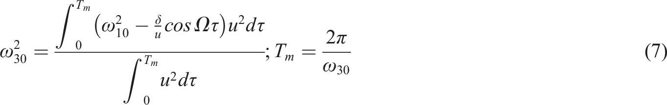
The numerical solution depicted in Figure 1 provides numerical confirmation for the comparison of equations (1) and (5). Calculation is performed for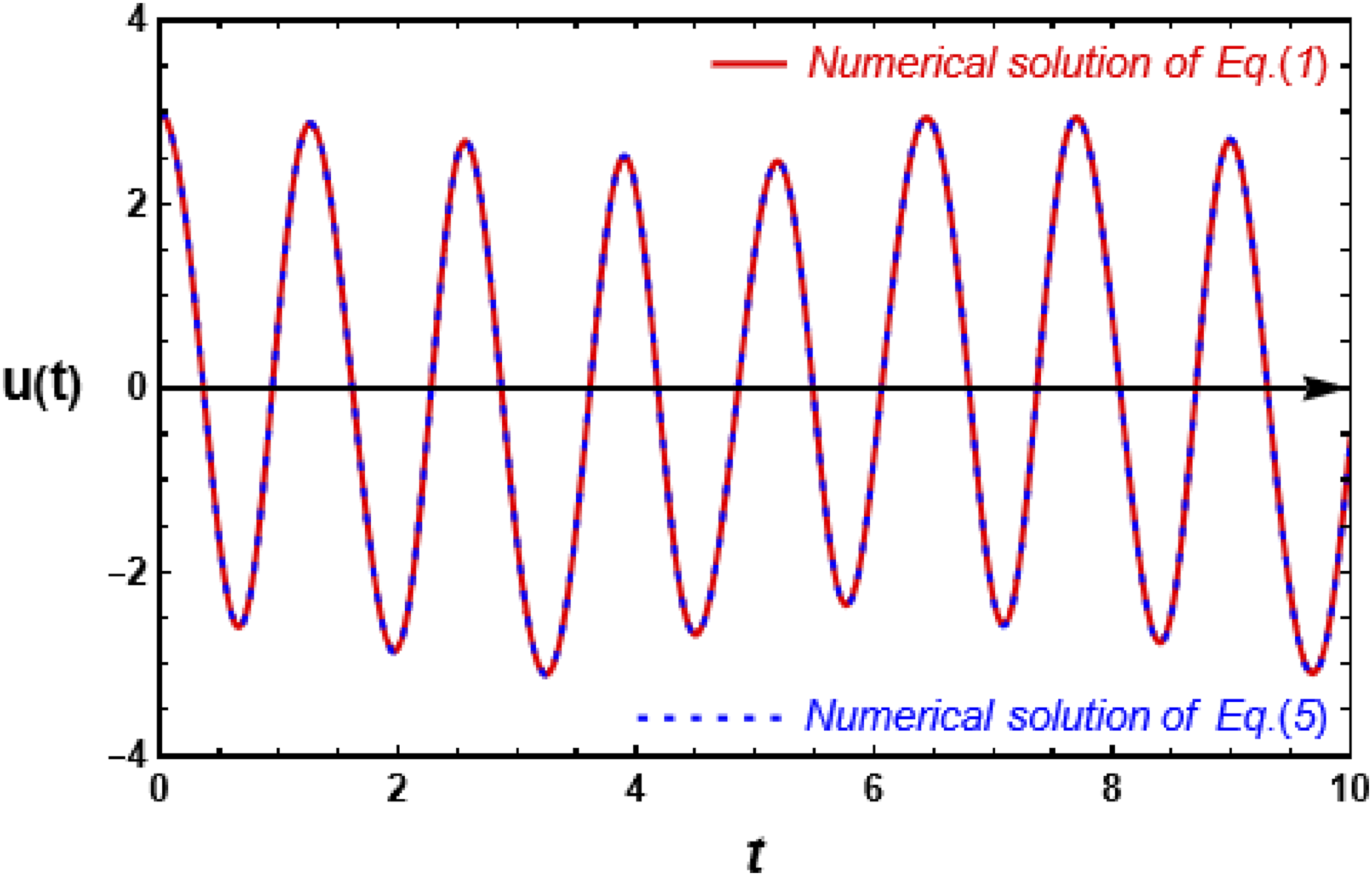

A = 3, B = 4, ω_{10} = 5, ω_{20} = 4, γ = 0.1, λ = 0.1, δ = 0 . 1, and σ = 1

Figure 1.

Illustrate the comparison of the numerical solution of equation (1) with the numerical solution of equation (5).

The graph shows that the two answers are in good agreement, with a relative error of 0.007131.

The mathematical representations of the modified 2-DOF system may take on a new shape in heterogeneous dynamical systems. Could perhaps have a fractal mathematical explanation for the 2-DOF system. As a result, the current study aims to investigate the modified 2-DOF system in fractal space via the Modified Lindstedt-Poincare transformation. Assuming that the fractional forms of the time-independent expression are

ω_{1} τ = t^{α}; 0 < α < \frac{1}{2}

(9)

ω_{2} τ = t^{β}; 0 < β < \frac{1}{2}

(10)

where

ω_{1}

and

ω_{2}

stand for the respective conservative frequencies of equations (5) and (2), respectively. For transformations (9) and (10), the time derivative should change into

\frac{d u}{d τ} = ω_{1} \frac{d u}{d t^{α}}, and \frac{d v}{d τ} = ω_{2} \frac{d v}{d t^{β}}

(11)

Using this approach, we have

u (τ) \to u (t^{α}) and v (τ) \to v (t^{β})

(12)

As a result, the second derivative’s transformation should become

\frac{d u}{d τ^{2}} = ω_{1}^{2} \frac{d u}{d t^{2 α}}, and \frac{d v}{d τ^{2}} = ω_{2}^{2} \frac{d v}{d t^{2 β}}

(13)

The following 2-DOF system in fractional form occurs when (11) and (13) are included into (5) and (2), respectively:

ω_{1}^{2} \frac{d u}{d t^{2 α}} + ω_{30}^{2} u - ω_{2} λ \frac{d v}{d t^{β}} + γ v = 2 u v

(14)

ω_{2}^{2} \frac{d v}{d t^{2 β}} + ω_{20}^{2} v + ω_{1} λ \frac{d u}{d t^{α}} + γ u = 2 u^{2}

(15)

Equations (14) and (15) follow He’s fractal derivative. He’s fractal derivative, introduced by Ji-Huan He, describes nonlocal, memory-dependent, and self-similar phenomena in physical and engineering systems, providing a generalized differential operator.^57–59 The fractal derivative presented by He is typically described as:

\frac{d f (t_{0})}{d t^{α}} = Γ (1 + α) \lim_{\begin{array}{l} t - t_{0} \to Δ t, \\ Δ t \neq 0 \end{array}} \frac{f (t) - f (t_{0})}{{(t - t_{0})}^{2}}

(16)

where

α

represents the fractal dimension and f(t) describes the physical phenomenon. This formulation varies from ordinary fractional derivatives (e.g., Riemann-Liouville or Caputo derivatives) in that it is scale dependent and designed specifically for fractal media and complicated geometries. It is noted that this fractal derivative has several qualities like the following:

\lim_{α \to 0} \frac{d f}{d t^{α}} = f, \lim_{α \to 1} \frac{d f}{d t^{α}} = \frac{d f}{d t}, and \lim_{α \to 2} \frac{d f}{d t^{α}} = \frac{d f}{d t^{2}}

(17)

The distinct fractal orders are associated with each equation. The orders, possibly written as α and β, affect the derivatives and overall behavior of equations. Understanding their roles is critical for manipulating equations efficiently. This work produces a generalized fractal nonlinear 2-DOF oscillator with two separate dimensions (α and β). This system has the following initial circumstances:

u (0) = A, \frac{d u (0)}{d t^{α}} = 0

(18)

v (0) = B, \frac{d v (0)}{d t^{β}} = 0

(19)

The nonlinear fractal system (14) and (15) can be seen as

ω_{1}^{2} \frac{d u}{d t^{2 α}} - ω_{2} λ \frac{d v}{d t^{β}} + f_{1} (u, v) u = 0

(20)

ω_{2}^{2} \frac{d v}{d t^{2 β}} + ω_{1} λ \frac{d u}{d t^{α}} + f_{2} (u, v) v = 0

(21)

where

f_{1} (u, v)

and

f_{2} (u, v)

are defined as

f_{1} (u, v) = ω_{30}^{2} + γ (\frac{v}{u}) - 2 v, and f_{2} (u, v) = ω_{20}^{2} + γ (\frac{u}{v}) - 2 (\frac{u^{2}}{v})

(22)

Follow the procedure proposed by El-Dib and Alyousef⁵⁴ to transform the nonlinear coupled systems (20) and (21) to the equivalent form shown below:

Introducing trial solutions for the nonlinear equations (20) and (21) utilizing the two scales technique, as

u_{0} = A \cos t^{α}; and v_{0} = B \cos t^{β}

(23)

The following expressions can be validated using the answers suggested here:

{\bar{U}}^{2} = \frac{1}{8 π} \int_{0}^{2 π} u_{0}^{2} (t^{α}) d t^{α} = \frac{A^{2}}{8}

(24)

{\bar{V}}^{2} = \frac{1}{8 π} \int_{0}^{2 π} v_{0}^{2} (t^{β}) d t^{β} = \frac{1}{8} B^{2}

(25)

where

{\bar{U}}^{2}

and

{\bar{V}}^{2}

are referred to as the mean-square displacements and velocities, respectively.

Apply the proposed trial solutions (23), using the mean squares provided by (24) and (25). The linearized form of the functions $f_{1} (u, v)$ and $f_{2} (u, v)$ is predicted to be

ω_{1}^{2} \equiv \lim_{u, v \to \bar{U}, \bar{V}} f_{1} = ω_{30}^{2} + γ (\frac{\bar{V}}{\bar{U}}) - 2 \bar{V} = ω_{30}^{2} + γ (\frac{B}{A}) - \frac{B}{\sqrt{2}}

(26)

ω_{2}^{2} \equiv \lim_{u, v \to \bar{U}, \bar{V}} f_{2} = ω_{20}^{2} + γ (\frac{\bar{U}}{\bar{V}}) - 2 (\frac{{\bar{U}}^{2}}{\bar{V}}) = ω_{20}^{2} + γ (\frac{A}{B}) - (\frac{A^{2}}{\sqrt{2} B})

(27)

Using (26) and (27), the equivalent linearization form for the system (20) and (21) may be found in the following form:

\frac{d u}{d t^{2 α}} + u = \frac{ω_{2}}{ω_{1}^{2}} λ \frac{d v}{d t^{β}}

(28)

\frac{d v}{d t^{2 β}} + v = - \frac{ω_{1}}{ω_{2}^{2}} λ \frac{d u}{d t^{α}}

(29)

Equations (28) and (29) represent the linearized versions of nonlinear equations (14) and (15), respectively. Numerical comparison may be valuable for validating the approach utilized in this investigation. In a specific circumstance, the two-scale description $t^{α} = t^{β} = T$ can be used to perform a full numerical investigation, confirming that both nonlinear and linear systems operate on the same timescale. The details of these calculations are as follows.

A = 0.1, B = 0.3, ω_{10} = 7, ω_{20} = 5, γ = 1, λ = 0.005, δ = 1, σ = 5

The results of these computations show an excellent agreement between the nonlinear system solutions and their linear equivalents, as shown in Figure 2. This alignment indicates that the linearization technique accurately captures the basic dynamics of the original nonlinear systems, proving the linear models’ validity for these particular equations. The relative error between equations (14) and (28) is projected to be 0.09595, indicating a difference of about. The relative error between equations (15) and (29) is calculated to be 0.06,107, indicating a smaller difference. This examination identifies discrepancies in accuracy or consistency between various sets of equations inside the mathematical model under consideration.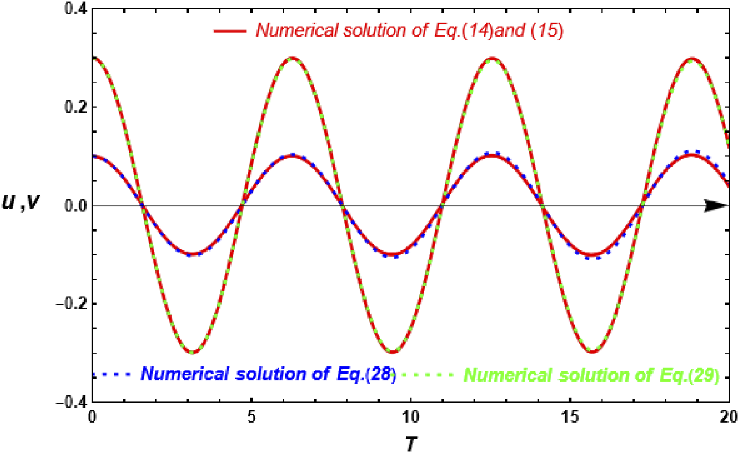

Figure 2.

Illustrate the comparison of the numerical solutions of equations (14) and (15) with the numerical solutions of equations (28) and (29), respectively.

An analytical solution for a dynamic system defined by equations (28) and (29) requires a systematic method that prepares the solutions for analysis in continuous space. This analysis will include non-resonance and internal resonance scenarios, which are critical for understanding the system’s stability and dynamic behavior under a variety of settings.

The non-resonance analysis

Non-resonance happens when the system’s frequencies are sufficiently separated so that the vibrational modes do not interact significantly. This spacing of frequencies prevents energy from quickly transferring between modes, which is a common cause of instability in systems with near frequencies (internal resonance). The following analysis solves systems (28) and (29) while accounting for the non-internal resonance case:

It is simple to show that equations (28) and (29) can be rewritten into a more understandable form, facilitating their solution:

\frac{d v}{d t^{β}} = \frac{ω_{1}^{2}}{ω_{2} λ} (\frac{d}{d t^{2 α}} + 1) u

(30)

\frac{d u}{d t^{α}} = - \frac{ω_{2}^{2}}{ω_{1} λ} (\frac{d}{d t^{2 β}} + 1) v

(31)

Addressing a system consisting of two connected fractal equations with distinct fractal orders is an intriguing mathematics challenge. Increasing the rank of fractal equations and effectively regulating the resulting system demands a thorough understanding of both the underlying mathematics and the physical or theoretical background. Completing these stages will increase the system’s complexity, allowing us to discover richer dynamics and more subtle insights into its behavior. To successfully elevate the rank of equations (30) and (31) and simplify their resolution or analysis, proceed as follows:

\frac{d}{d t^{β}} (\frac{d v}{d t^{β}}) = \frac{ω_{1}^{4}}{ω_{2}^{2} λ^{2}} {(\frac{d}{d t^{2 α}} + 1)}^{2} u

(32)

\frac{d}{d t^{α}} (\frac{d u}{d t^{α}}) = \frac{ω_{2}^{4}}{ω_{1}^{2} λ^{2}} {(\frac{d}{d t^{2 β}} + 1)}^{2} v

(33)

Convert each equation to a standard form that reveals its underlying structure. For second-order differential equations, this often entails arranging them so that they exhibit terms proportional to the displacement (or fundamental variable of the system), its first derivative (velocity), and its second derivative (acceleration). To speed up and simplify the mathematical process of solving fractal equations (32) and (33) one might convert it into an equivalent system that simulates the continuous medium. To attain this goal, we must follow El-Dib and Nasser’s bridge.^54–56 Thus, it is possible to achieve the aims with the following adapters:

\frac{d . .}{d t^{S}} = P^{S - 1} \sin (\frac{1}{2} π S) \frac{d . .}{d t} + P^{S} \cos (\frac{1}{2} π S) . .; 0 < S < 1

(34)

where P is a non-dimensional parameter that denotes certain functions in

α

and

β,

S is a moving rank. The following expression is sufficient:

\frac{d . .}{d t^{2 S}} = (P^{2 S - 2} \sin^{2} (\frac{1}{2} π S) \frac{d^{2} . .}{d t^{2}} + 2 P^{2 S - 1} \sin (\frac{1}{2} π S) \cos (\frac{1}{2} π S) \frac{d . .}{d t} + P^{2 S} \cos^{2} (\frac{1}{2} π S) . .)

(35)

Adding (34) and (35) to (32) and (33) results in the continuous space as

\ddot{u} + 2 P η_{1} \dot{u} + P^{2} η_{1}^{2} u = P ξ_{2} \dot{v} + P^{2} ζ_{2} v

(36)

\ddot{v} + 2 P η_{2} \dot{v} + P^{2} η_{2}^{2} v = P ξ_{1} \dot{u} + P^{2} ζ_{1} u

(37)

This is a linearly connected damping system with two variables: u(t) and v(t). The coefficients present in the aforementioned system are stated below:

η_{1} = \frac{1 + P^{2 α} \cos (π α)}{P^{2 α} \sin (π α)}, η_{2} = \frac{1 + P^{2 β} \cos (π β)}{P^{2 β} \sin (π β)}

ξ_{1} = \frac{ω_{1}^{2} λ^{2} P^{2 α} \sin (π α)}{ω_{2}^{4} P^{4 β} \sin^{2} (π β)}, ξ_{2} = \frac{ω_{2}^{2} λ^{2} P^{2 β} \sin (π β)}{ω_{1}^{4} P^{4 α} \sin^{2} (π α)}, ζ_{1} = \frac{ω_{1}^{2} λ^{2} P^{2 α} \cos (π α)}{ω_{2}^{4} P^{4 β} \sin^{2} (π β)}, ζ_{2} = \frac{ω_{2}^{2} λ^{2} P^{2 β} \cos (π β)}{ω_{1}^{4} P^{4 α} \sin^{2} (π α)}

(38)

To work in the continuous space, we must apply the transformation (34) to the initial conditions (18) and (19), which have the following form:

u (0) = A, \dot{u} (0) = - A P \cot (\frac{1}{2} π α)

(39)

v (0) = B, \dot{v} (0) = - B P \cot (\frac{1}{2} π β)

(40)

To manage the coupled system given by equations (36) and (37), it is fair to express the relationship between the variables u(t) and v(t) using the following correlation relationship:

v (t) = χ u (t)

(41)

where χ is a real constant parameter that can be calculated by comparisons. This method includes defining a functional connection in which u(t) and v(t) are directly stated as functions of χ. This correlation allows for a more streamlined analysis by simplifying the system to a single functional dependency. This expression will aid in the derivation of solutions and further analysis by allowing the substitution of this relationship into one of the linked equations, potentially reducing the system to a single equation involving one variable. Simplicity is crucial for solving complex dynamic systems and understanding variable interaction over time.

Applying equation (41) to equations (36) and (37) creates an uncoupled system by replacing v(t) with u(t), reducing equations to expressions in terms of u(t) and its derivatives, and reducing each equation to a single variable, u(t). This reduction simplifies system analysis and solution by focusing on the dynamics of a single variable rather than directly dealing with coupled interactions. This method may allow for direct integration or solution approaches applicable to single variable differential equations. Here’s how the equations might appear after transformation:

\ddot{u} + P (2 η_{1} - χ ξ_{2}) \dot{u} + P^{2} (η_{1}^{2} - χ ζ_{2}) u = 0

(42)

Modified equation (37) can also be reduced to a form that either acts as a redundant check on the solution produced by Modified equation (36) or gives an independent avenue to solve for v(t). The first strategy is analyzed to identify the unknown χ.

\ddot{u} + \frac{P}{χ} (2 χ η_{2} - ξ_{1}) \dot{u} + \frac{P^{2}}{χ} (χ η_{2}^{2} - ζ_{1}) u = 0

(43)

Damped oscillations occur in a variety of natural environments. It happens when a system attempts to reach equilibrium but is constantly interrupted by an external stimulus. Damped oscillations occur when energy is lost owing to frictional resistance. There are three types of damping: critical, underdamped, and overdamped. Underdamped systems have less friction; therefore, the item will continue to oscillate about the equilibrium position, but the magnitude of the oscillations will decrease over time. Critical damping occurs when the frictional force is sufficient to stop the vibration. A critically damped system returns to equilibrium as quickly as possible without fluctuation. Overdamped systems have high friction, forcing them to move slowly to their equilibrium position without fluctuating.

As a result, the uncoupling process gives a clearer path to solution discovery and subsequent dynamic analysis of the system. This formulation enables us to directly assess how changes in u(t) and their rates of change affect the system’s frequency, providing critical insights into the system’s dynamic behavior. It’s especially beneficial for understanding oscillatory dynamics and stability criteria in differential equation-modeled systems. The actual form of the system’s frequencies would be determined by its characteristics and properties.

Equations (42) and (43) are two second-order equations for the same variable with different damping coefficients and natural frequencies, resulting in two different frequencies Θ₁ and Θ₂. The frequency relationship that regulates the single variable equation (42) is as follows.

Θ_{1}^{2} = P^{2} (η_{1}^{2} - χ ζ_{2} - \frac{1}{4} {(2 η_{1} - χ ξ_{2})}^{2})

(44)

In contrast, the frequency connection that drives equation (43) can be expressed as

Θ_{2}^{2} = \frac{P^{2}}{χ^{2}} (χ (χ η_{2}^{2} - ζ_{1}) - \frac{1}{4} {(2 χ η_{2} - ξ_{1})}^{2})

(45)

To maintain stable oscillatory behavior, the frequency values computed from equations (44) and (45) must be positive. Positive squared frequencies usually imply that a system recovers to equilibrium following a disturbance, rather than deviating away from it. The frequency descriptions provided in equations (44) and (45) can be used to ensure that the system meets its stability requirements. To keep the system stable, both equations must have positive right-hand sides. This requirement suggests that the frequencies defined by the equations help to stabilize the system’s dynamics. The basic prerequisite for stability in a non-internal resonance situation is sufficient frequency separation. This separation must be sufficient to prevent significant coupling of modes, which can lead to an exponential increase in response in one or more modes.

To preserve system stability, it is necessary to ensure that both equations (44) and (45) provide positive outcomes. These requirements should be extensively evaluated and validated as follows:

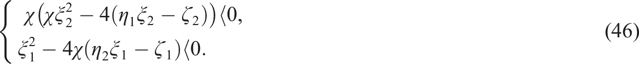
{\begin{cases} χ (χ ξ_{2}^{2} - 4 (η_{1} ξ_{2} - ζ_{2})) 〈 0, \\ ξ_{1}^{2} - 4 χ (η_{2} ξ_{1} - ζ_{1}) 〈 0 . \end{cases}

(46)

These criteria ensure that for all positive values of the parameter χ, the system is stable, meaning it returns to equilibrium after any perturbation and does not exhibit unbounded or increasing behavior.

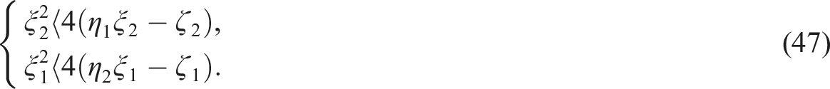
{\begin{cases} ξ_{2}^{2} 〈 4 (η_{1} ξ_{2} - ζ_{2}), \\ ξ_{1}^{2} 〈 4 (η_{2} ξ_{1} - ζ_{1}) . \end{cases}

(47)

Combining many stability requirements into a single, more complete condition can frequently simplify analysis and increase practical applicability. It is advised that the unified conditions (47) be simplified to the greatest extent possible to ensure that they remain valid and that no critical elements of the particular requirements are lost in the process. This is usually performed by combining the conditions into a single mathematical expression with logical operators. Consider how the stability conditions given by (47) can be combined into a single all-encompassing stability criterion.

(ξ_{2}^{2} - 4 (η_{1} ξ_{2} - ζ_{2})) (ξ_{1}^{2} - 4 (η_{2} ξ_{1} - ζ_{1})) > 0

(48)

When considering dynamic system stability, especially in contexts involving resonance, the non-internal resonance scenario is an important criterion for establishing stability. This context relates to instances where the two frequencies Θ₁ and Θ₂ of the system do not align or match closely, therefore avoiding problems connected with resonance events.

The solution of equation (42) can be provided in the form

u (t) = e^{- \frac{1}{2} P (2 η_{1} - χ ξ_{2}) t} (A \cos Θ_{1} t + \frac{A P}{2 Θ_{1}} (2 η_{1} - χ ξ_{2} - 2 \cot (\frac{1}{2} π α)) \sin Θ_{1} t)

(49)

To derive the solution for the variable v(t) we may return to the modified form of equation (37) and solve it using (41) yielding

v (t) = e^{- \frac{1}{2} \frac{P}{χ} (2 χ η_{2} - ξ_{1}) t} (B \cos Θ_{2} t + \frac{B P}{2 χ Θ_{2}} (2 χ η_{2} - ξ_{1} - 2 χ \cot (\frac{1}{2} π β)) \sin Θ_{2} t)

(50)

To estimate the unknown parameter χ, proceed as follows:

Given that equations (42) and (43) are damped second-order homogeneous equations for the variable u(t), there are likely expressions with identical frequency components. Thus, equating the right-hand sides of (44) and (45) implies:

χ^{4} ξ_{2}^{2} + 4 χ^{3} (ζ_{2} - η_{1} ξ_{2}) - 4 χ (ζ_{1} - η_{2} ξ_{1}) - ξ_{1}^{2} = 0

(51)

This equation frequently produces a link between the coefficients of the two equations, implying that an important condition must be met for the solutions u(t) of both equations to be consistent.

Numerical validation and discussion for the non-internal resonance case

To validate theoretical results, they must be compared to numerical solutions. Specific constants for the coefficients are incorporated into the original system to assist the computations, which are shown as

A = 1, B = 3, ω_{10} = 5, ω_{20} = 3, γ = 1, λ = 0.3, δ = 1, σ = 5, P = 0.1, α = 0.4, β = 0.3

Figures 3(a)–(c) compare the analytical solutions provided in equations (49) and (50) to the numerical solutions obtained from equations (36) and (37). The results show a remarkable similarity between the two approaches:

• The relative error for analytical solution (49) is 0.003059, 0.009978 and 0.004844.

• The analytical solution (50) has a relative error (0.001684, 0.002263 and 0.001203).

Figure 3.

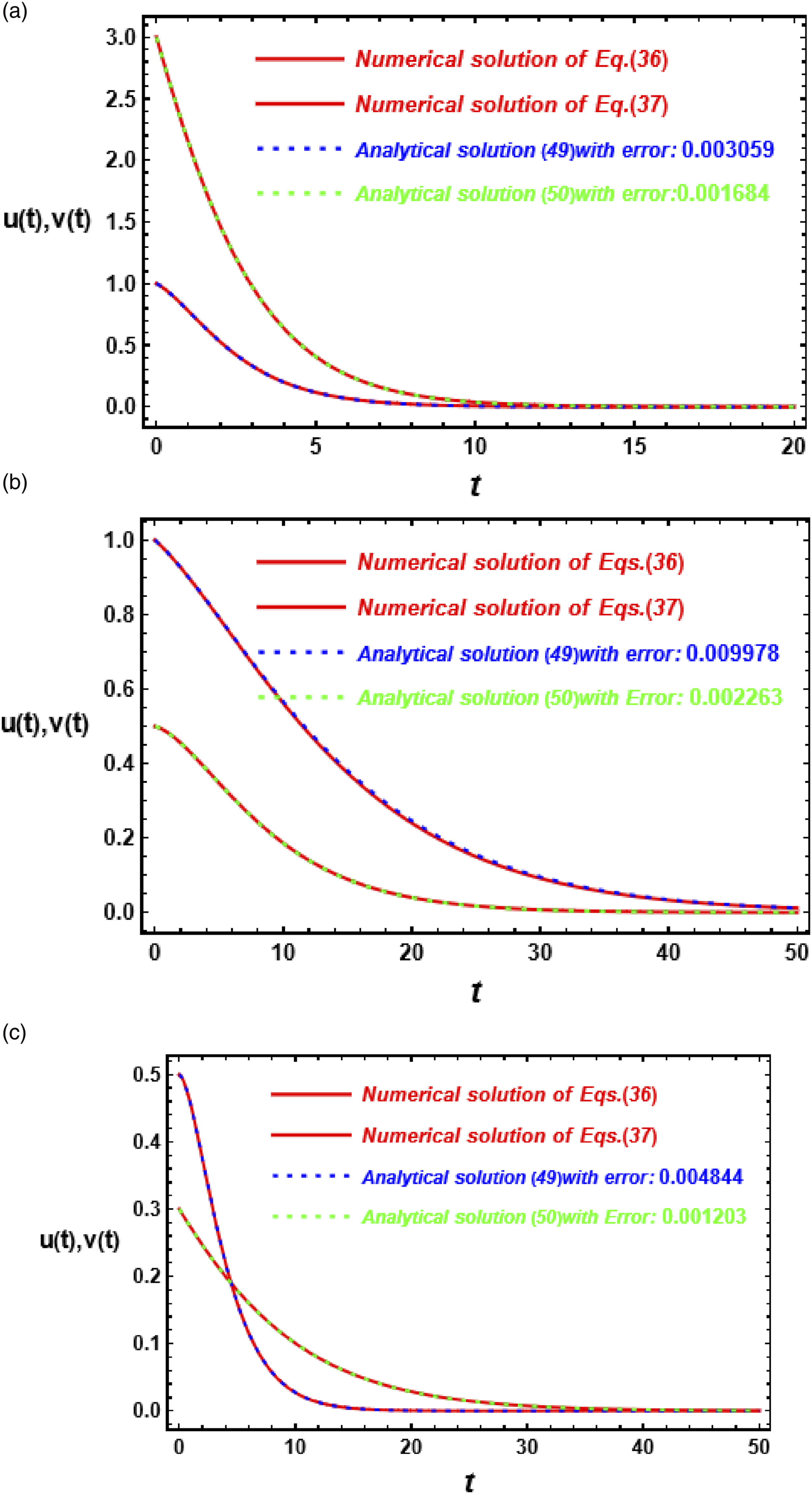
(a): Compare the numerical solutions of equations (36) and (37) to the analytical solutions found in (49) and (50) for a system of $A = 1, B = 3, ω_{10} = 5, ω_{20} = 3, γ = 1, λ = 0.1, δ = 1, σ = 5, P = 0.1, α = 0.4, β = 0.2 .$ (b): Compare the numerical solutions of equations (36) and (37) to the analytical solutions found in (49) and (50) for a system of $A = 1, B = 0.5, ω_{10} = 2, ω_{20} = 5, γ = 2, λ = 0.3, δ = 5, σ = 20, P = 0.01, α = 0.2, β = 0.3 .$ (c): Compare the numerical solutions of equations (36) and (37) to the analytical solutions found in (49) and (50) for a system of $A = 0.5, B = 0.3, ω_{10} = 7, ω_{20} = 5, γ = 3, λ = 0.2, δ = 3, σ = 30, P = 0.015, α = 0.4, β = 0.1 .$

These low relative errors show that the analytical answers are more accurate than their numerical counterparts, implying that the analytical methods are reliable under the conditions evaluated. Figure 3 further indicates that the solution’s behavior does not oscillate over time. This lack of oscillatory activity contrasts sharply with the behaviors depicted in Figure 2, which shows oscillations in the absence of damping using a two-scale approach. Figures 3(a)–(c) show an overdamped response as a direct effect of translating the system into continuous space. This overdamped nature results from the inclusion of fractal characteristics in the damping coefficients, which introduce significant resistance, successfully suppressing oscillations in both the numerical and analytical models.

These findings highlight the need to take fractal factors into account when modeling and analyzing dynamic systems in continuous space. The excellent correlation between analytical and numerical results not only verifies the mathematical models but also boosts confidence in their usage for future research or practical applications, especially in systems where damping and stability are essential elements.

Figure 4 depicts a plot of the stability condition (48) in the non-internal resonance situation, showing stable and unstable zones in the plane (α-β) for various parameter P values. The computation was carried out using the same system as shown in Figure 3. Two unstable zones and one stable region have been observed. Stability is seen on the line α + β = 0 and its surroundings. As α and β increased concurrently, the stable zone stretched beyond the line α + β = 0. It is revealed that increasing P reduces the stability zone while increasing the instability zone.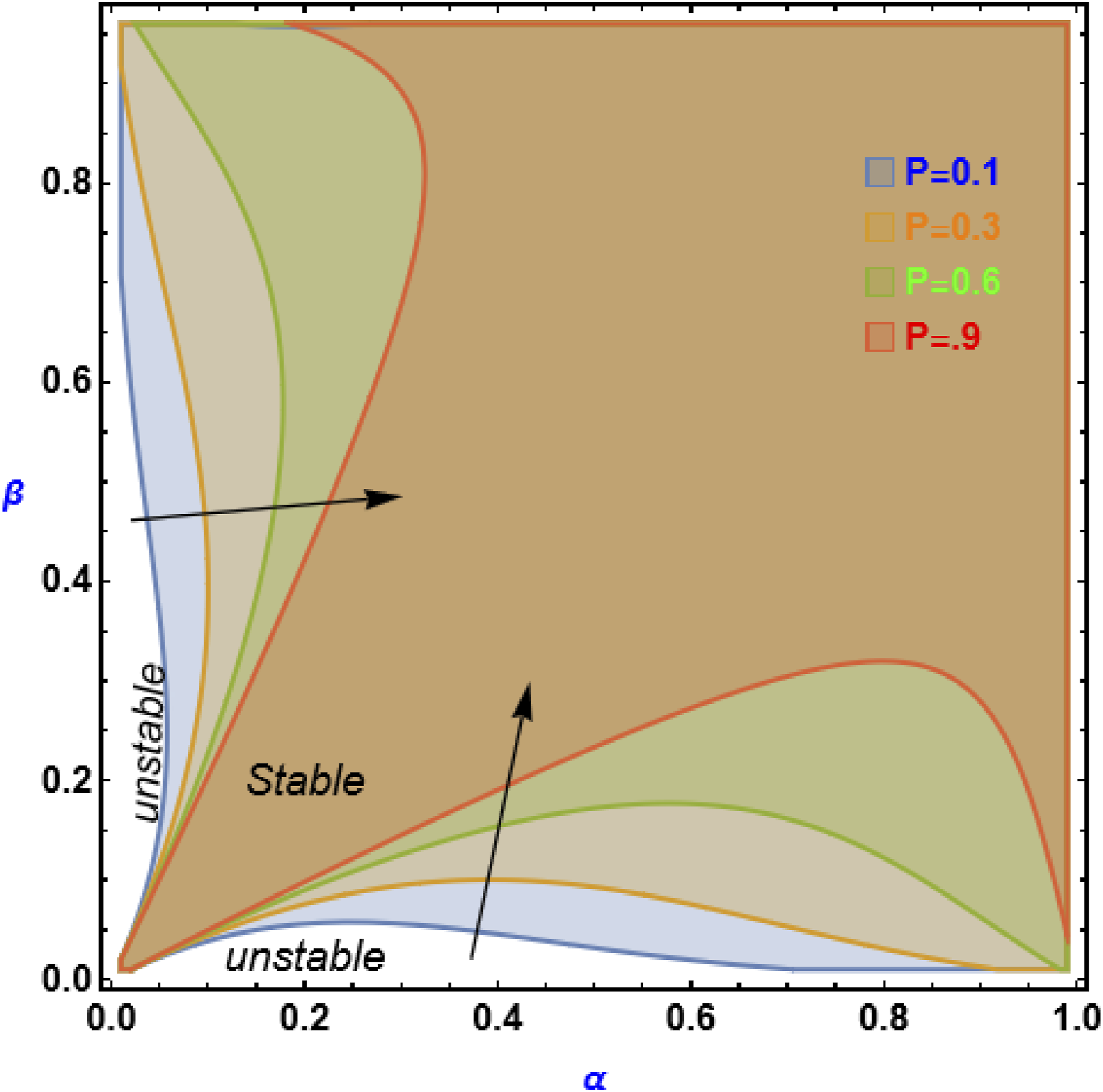

Figure 4.

The graph depicts the stability criteria (46) in the plan (β - α) as the parameter P varies for the same system as in Figure 3.

Figure 5 shows the stability behavior of the plane (δ-σ) with increasing amplitude A. In this graph, condition (46) is derived for the system.

B = 0.3, ω_{10} = 2, ω_{20} = 1, λ = 0.001, α = 0.4, β = 0.4, γ = 1; P = 0.1

Figure 5.

The graph depicts the stability criteria (46) in the plan (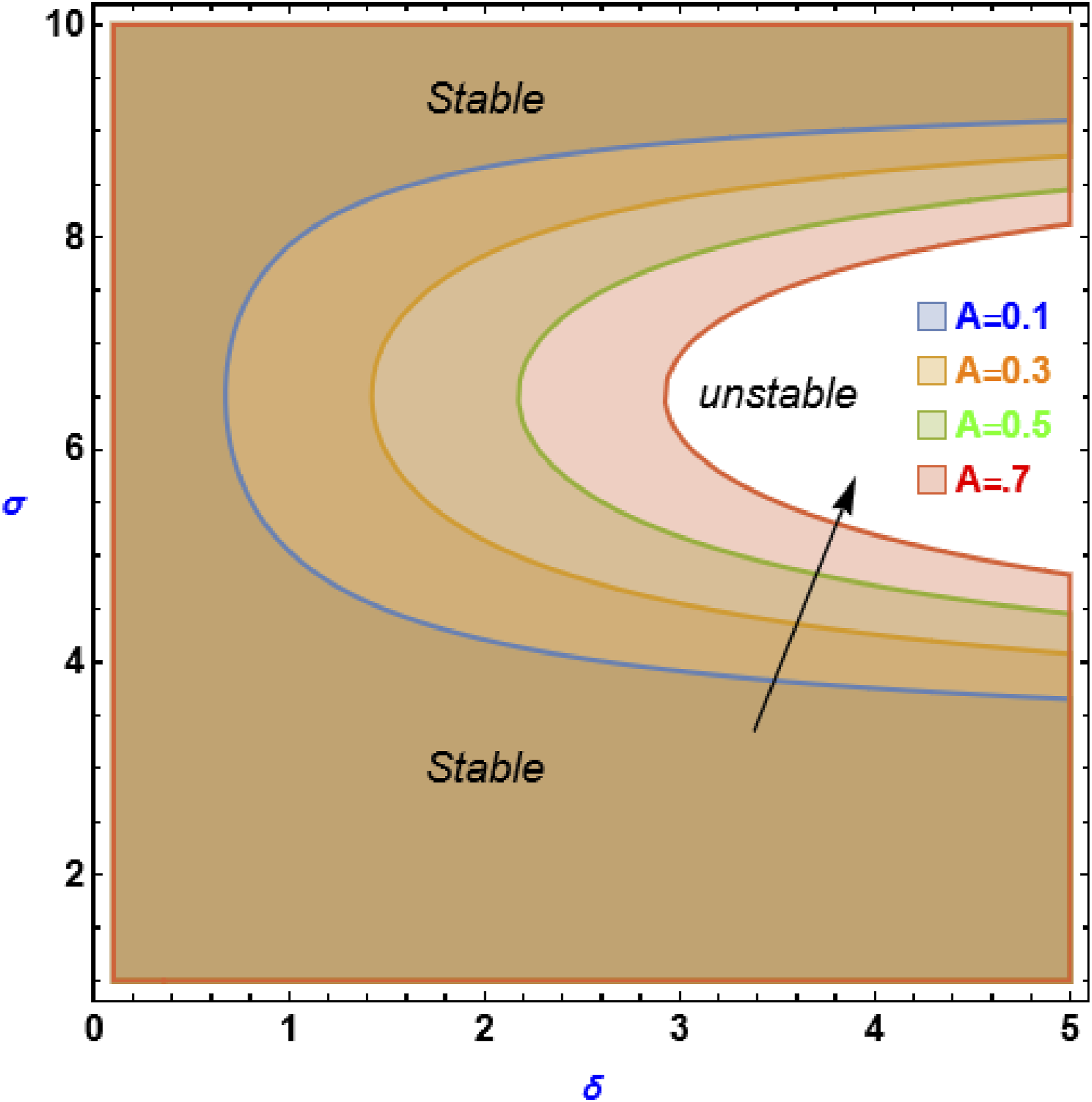 $δ - σ$ ) with a variation of the amplitude A for the system $B = 0.3, ω_{10} = 2, ω_{20} = 1, λ = 0.001, α = 0.4, β = 0.4, γ = 1; P = 0.1$

The graph shows that the unstable zone is bounded by a stable sector. The unstable region starts at σ = 6.5. The harmonic resonance zone shrinks as amplitude A grows. It should be noted that the stable zone occurred for tiny P values. When p is increased to p > 0.3, a substantial dramatic change happens, causing the stable zone to become an unstable area and the interior to become stable, that is, the roles are reversed, as illustrated in Figure 6. In this case, increasing amplitude A reverses its role, resulting in an unstable influence.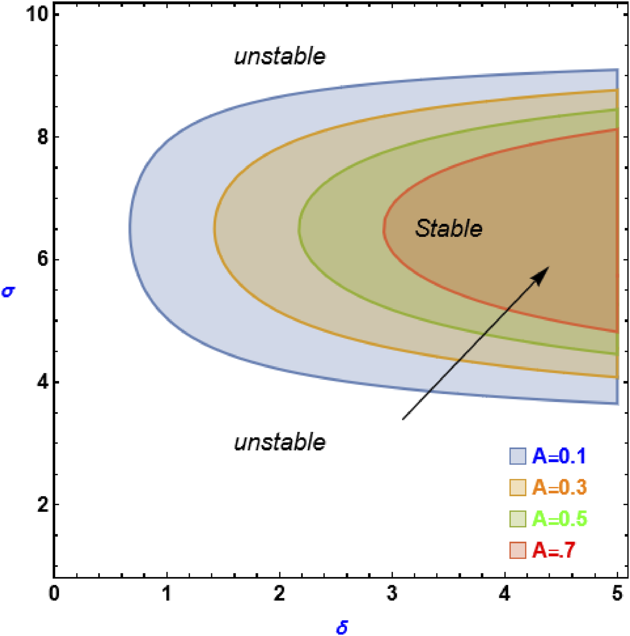

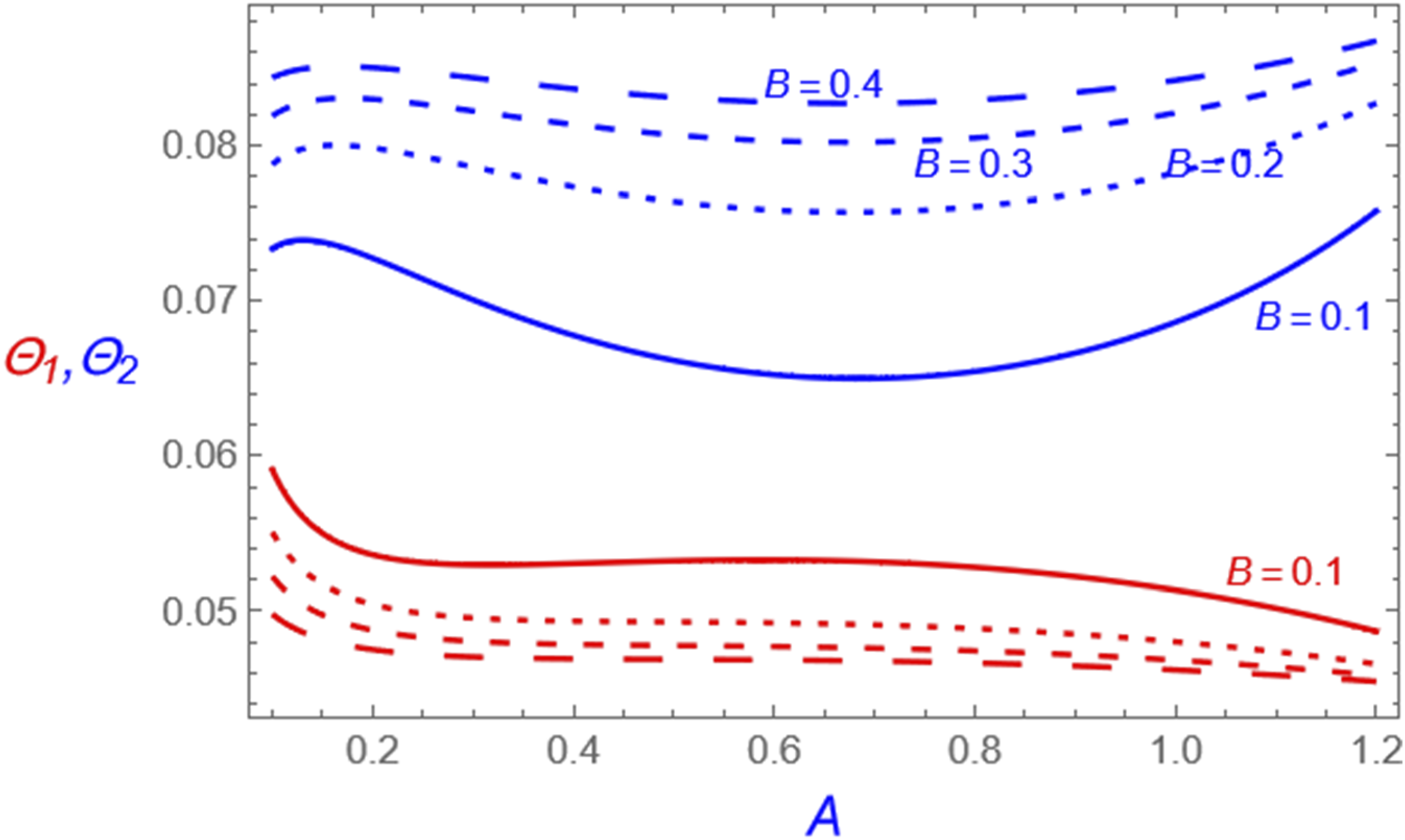
Figure 6.

The graph represents the stability requirements (46) in the plan (δ−σ) with variation of the amplitude A for the same system provided in Figure 5, except that the parameter p changes to the value p = 0.31.

Figures 7 and 8 illustrate the relationship between frequencies Θ₁ and Θ₂ and oscillation amplitudes for the system in Figure 3(a) except that $α = 0.5, β = 0.4$ . However, in these graphs, both frequencies are plotted versus amplitude A with varying amplitude B in the plane of (Θ₁, Θ₂−A). In these graphs, frequency Θ₁ is represented by red solid and dashed curves, whereas frequency Θ₂ is represented by blue solid and dashed curves. Figure 7 illustrates a series of very small amplitude B values, while Figure 8 investigates the effect of changing relatively larger amplitude B values. Figure 7 illustrates that the Θ1 curve is placed above the Θ₂ curve. The Θ₁ curve is a critical indicator for identifying stable and unstable states. Figure 8 demonstrates that as B values increase, the Θ₁ curve shifts downward while the Θ₂ curve rises, indicating a change in system behavior. In Figure 8, the critical curve (Θ₂ curve) transforms into the transition curve. This study examines how amplitude variations affect the system’s frequency response and stability characteristics, revealing more about the system’s nonlinear nature.

Figure 7.

Graphic the relation between the frequencies Θ₁ and Θ₂ versus the amplitude A for variation of very amplitude B (B = 0.01, 0.02, 0.03, and 0.04).

Figure 8

Graphic the relation between the frequencies Θ₁ and Θ₂ versus the amplitude A for variation of very amplitude B (B = 0.1, 0.2, 0.3, and 0.4).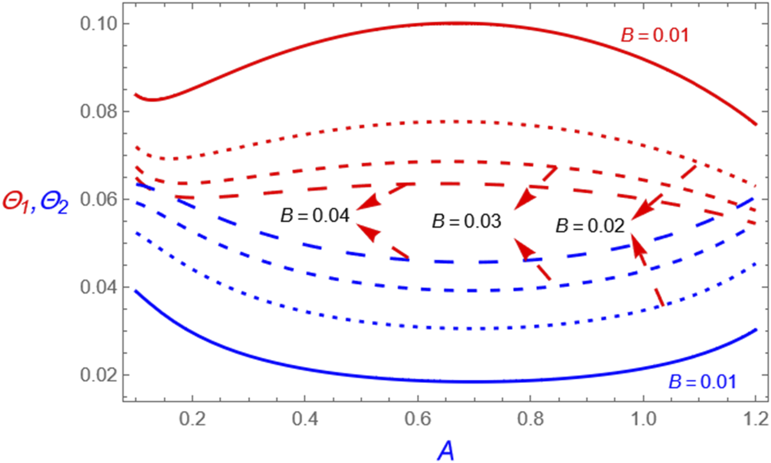

Common frequency approach (internal resonance case)

Internal resonance is the synchronization of frequencies, which can significantly increase the system’s reaction. Because of the possibility of strong interactions between modes, dealing with internal resonance in dynamic systems is significantly more complex than dealing with non-internal resonance. Internal resonance happens when the system’s two frequencies become commensurate, which means they are integer multiples or near ratios of one another. This can result in massive energy exchanges between the modes, potentially causing huge amplitude oscillations that jeopardize the system’s stability internal resonance management involves design methods, increased damping, and active control measures to strengthen systems, ensure safety, improve performance, and improve reliability.

To create an uncoupled system with a common frequency Θ, simplify the system into a single equation governing one variable. This involves minimizing coupled equation complexity and isolating the system’s dynamics, often by expressing one variable in terms of another or removing secondary variables. Here’s how it can be done:

Eliminating the variable v(t) from equation (30) with the help of equation (31) provides

(\frac{d}{d t^{2 α + 2 β}} + \frac{1}{ω_{1} ω_{2}} λ^{2} \frac{d}{d t^{α + β}} + \frac{d}{d t^{2 α}} + \frac{d u}{d t^{2 β}} + 1) (u, v) = 0

(52)

Because there is only one variable, the ensuing equation (52) is simple to solve. It can be approached using the traditional techniques for solving ordinary differential equations. These equations appear to be extremely challenging and cannot be solved using the two-scale approach. By simplifying the system to a single equation governing one variable with a constant frequency, the analysis becomes more intelligible, and mathematical modeling insights can be applied more directly to understand and regulate the system. Analyze the simplified equations by putting them into continuous space. For instance, combining (34) and (35) with (52) results in

\ddot{u} + P μ \dot{u} + P^{2} ϖ^{2} u = 0

(53)

\ddot{v} + P μ \dot{v} + P^{2} ϖ^{2} v = 0

(54)

Equations (53) and (54) are second-order homogeneous differential equations with damping that share the same damping coefficient and natural frequency. This closeness implies a unified approach to their study and potential solutions. Understanding that both equations have the same dynamic properties enables more efficient control strategies and optimization techniques, particularly in engineering applications requiring accurate motion control. In practice, if these equations reflect physical systems like mechanical or electrical systems, the same damping and frequency parameters indicate that they have equivalent dynamic properties. This is particularly beneficial in synchronized systems or situations that demand consistent dynamic behavior across multiple components.

The coefficients in equations (53) and (54) are as follows:

μ = 2 \cot (\frac{1}{2} π α + \frac{1}{2} π β) + \frac{P^{2 α} \sin (π α) + P^{2 β} \sin (π β)}{P^{2 α + 2 β} \sin^{2} (\frac{1}{2} π α + \frac{1}{2} π β)} + \frac{1}{ω_{1} ω_{2}} \frac{λ^{2}}{P^{α + β} \sin (\frac{1}{2} π α + \frac{1}{2} π β)}

(55)

ϖ^{2} = \cot^{2} (\frac{1}{2} π α + \frac{1}{2} π β) + \frac{P^{2 α} \cos (π α) + P^{2 β + 2} \cos (π β)}{P^{2 α + 2 β} \sin^{2} (\frac{1}{2} π α + \frac{1}{2} π β)} + \frac{λ^{2} P^{α + β} \cos (\frac{1}{2} π α + \frac{1}{2} π β) + ω_{1} ω_{2}}{ω_{1} ω_{2} P^{2 α + 2 β} \sin^{2} (\frac{1}{2} π α + \frac{1}{2} π β)}

(56)

Equations (53) and (54) generate the same solutions. Because both equations have the same coefficients, they can be explored with the same techniques. Furthermore, they can be studied and manipulated at the same rate. The system’s similar qualities make it simple to assess how it responds to various initial conditions or external inputs. Depending on the situation’s specific requirements and constraints, common methods for solving second-order linear differential equations can be used. The answers are as follows:

u (t) = A e^{- \frac{1}{2} P μ t} (\cos Θ t + \frac{P}{2 Θ} (μ - 2 \cot (\frac{1}{2} π α)) \sin Θ t)

(57)

v (t) = B e^{- \frac{1}{2} P μ t} (\cos Θ t + \frac{P}{2 Θ} (μ - 2 \cot (\frac{1}{2} π β)) \sin Θ t)

(58)

where the frequency Θ is given by

Θ^{2} = P^{2} (ϖ^{2} - \frac{1}{4} μ^{2})

(59)

It is necessary to validate this criterion with numerical data. Before beginning the numerical calculations, we must first estimate the unknown parameter P. This can be performed by comparing the coefficients of national frequency in equations (52) and (53). The parameter P has the following relationship.

P^{2} = \frac{P^{2 α + 2 β} \sin^{2} (\frac{1}{2} π α + \frac{1}{2} π β) - P^{2 α + 2} \cos (π α) - P^{2 β + 2} \cos (π β)}{1 + P^{2 α + 2 β} (\cos (\frac{1}{2} π α + \frac{1}{2} π β) + \frac{1}{ω_{1} ω_{2}} λ^{2}) \cos (\frac{1}{2} π α + \frac{1}{2} π β)}

(60)

As shown, equation (60) is in a transcendental form for the unknown P, which should be solved numerically.

Validating simplified model equations (53) and (54) against analytical solutions (57) and (58) is crucial for guaranteeing model accuracy and reliability. Figure 9 depicts the same layout as in Figure 3. This assures consistency in the settings used to test the models. Unlike in Figure 3, the parameter P is computed numerically using equation (60). This provides more accurate input to the models based on the present system conditions. Inspection Figure 9 ensures that the simplifications used throughout the modeling process did not ignore critical features of the system’s behavior, as seen in Figure 3. The numerical models and analytical solutions have excellent agreement, with relative errors of 1.073 × 10−7 and 1.067 × 10−7, respectively. This ensures the overdamping behavior stays functional.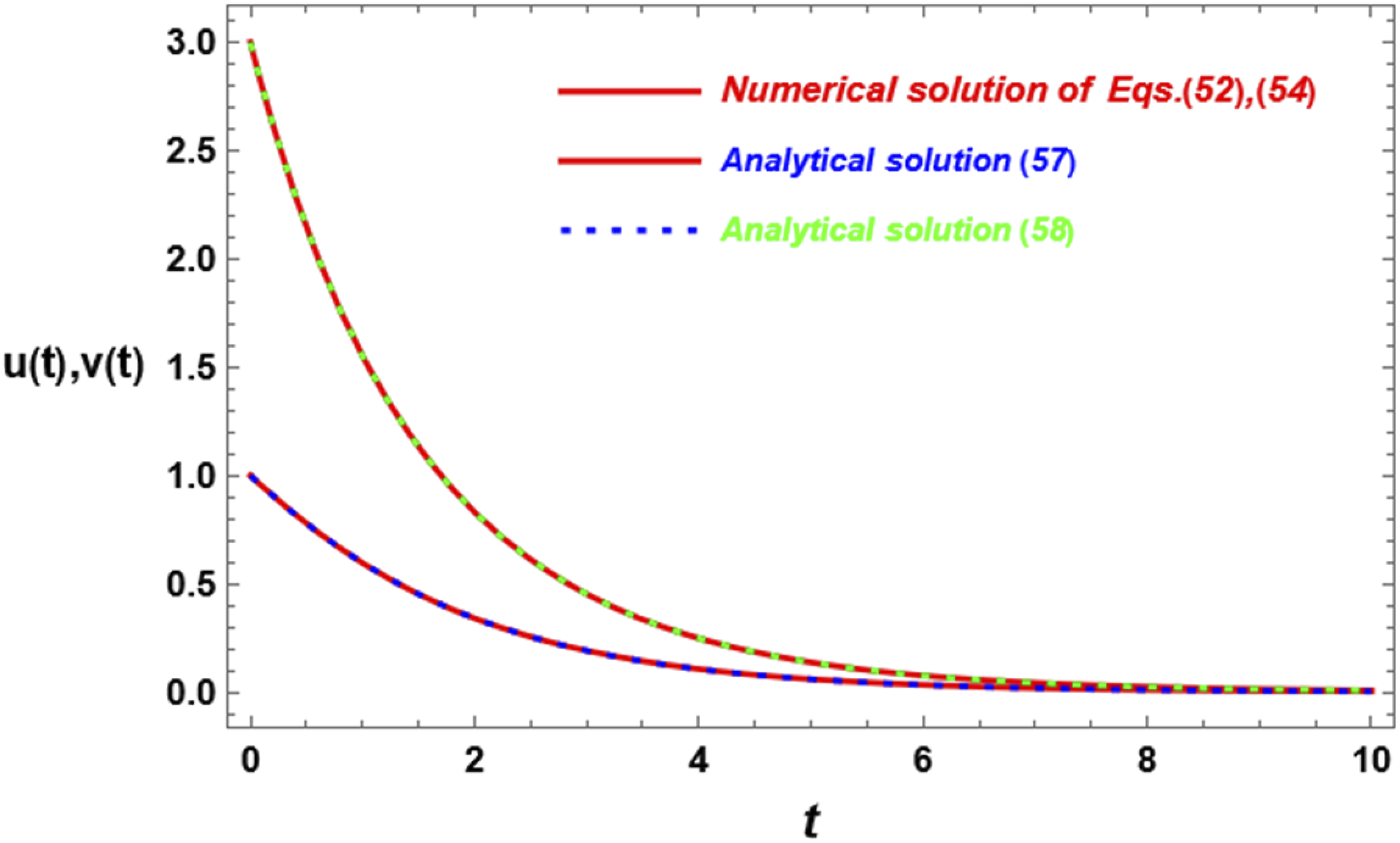

Figure 9.

Compare the numerical solutions of equations (53) and (54) to the analytical solutions found in (57) and (58) for the same system studied in Figure 3, except that the parameter P has been calculated from equation (60).

Analysis of stability and behavior in the internal resonance case

Solutions (57) and (58) with real Θ values indicate a stable system with no complex or divergent behavior. For this to be true, several conditions must be followed to ensure that the solutions stay genuine and limited. Typically, this means that the discriminant of the characteristic equation produced from the differential equation is not negative. To verify that the solutions are stable and actual, the following requirements can be structured:

ϖ^{2} - \frac{1}{4} μ^{2} > 0 and μ > 0

(61)

Numerical illustration and stability discussion

This section explored a system’s stability behavior under internal resonance conditions, using a specific set of stability requirements (most likely equation (61)). The system under consideration is identical to the one depicted in Figure 4, permitting a comparison of the two scenarios. The study explains the stability behavior in the (α−β) plane, as illustrated in Figure 10. Variations in the parameter P alter the stability areas, as illustrated in this graph. The graph shows an unstable area at the line α + β = 0. This region divides the stable area into two distinct sections, which differs from the behavior seen in Figure 4. This demonstrates a notable difference in behavior between internal and non-internal resonance settings. In the internal resonance situation, α = β creates instability. However, in the non-internal resonance situation, this condition becomes stable. The graph shows that when the parameter P increases, the unstable zone widens, which is consistent with the findings in Figure 4. Internal resonance and non-internal resonance scenarios have distinct stability behaviors, with the requirement α = β playing a unique role in each. The influence of parameter P is also consistent with the expected results from previous observations.

Figure 10.

Show the stability graph of the internal resonance scenario in the plane (α−β) for different parameters p values for the identical system as in Figure 4.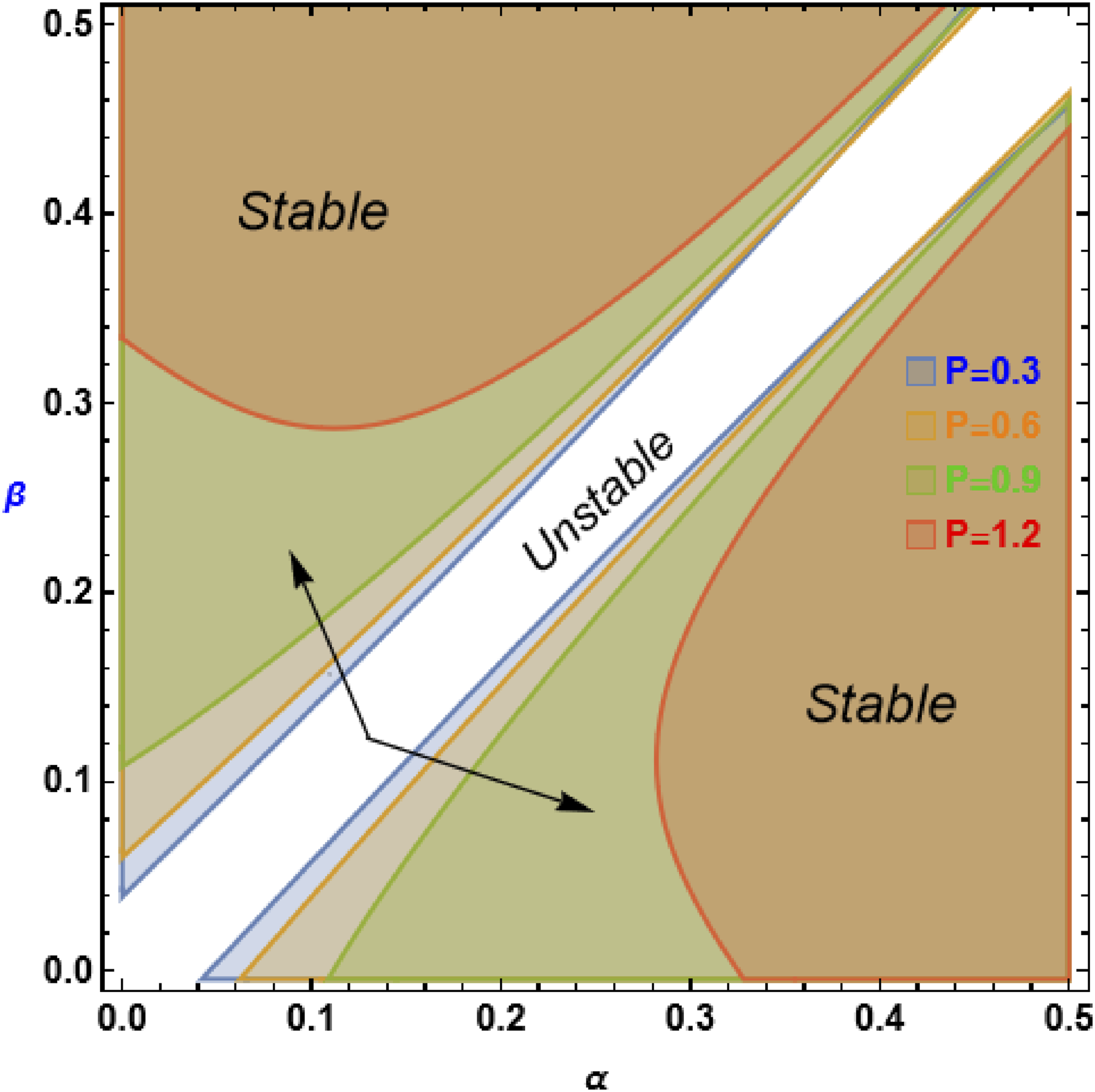

Figure 11 depicts the stability behavior on the (λ−α) plane, emphasizing the interaction of fractal orders β and α. The graph shows that when β approaches α, an unstable zone forms between stable zones. This shows that the proximity of β and α in the stability plane leads to instability. As β approaches α, an unstable zone emerges, imitating resonance behavior. This effect, known as “fractal resonance,” stresses the necessity of fractal organization in maintaining system stability. The convergence of β and α causes instability, highlighting the role of fractal resonance in the system’s stability dynamics. This results in patterns of instability that are comparable to classical resonance scenarios.

Figure 11.

Illustrate the stability behavior in the plane (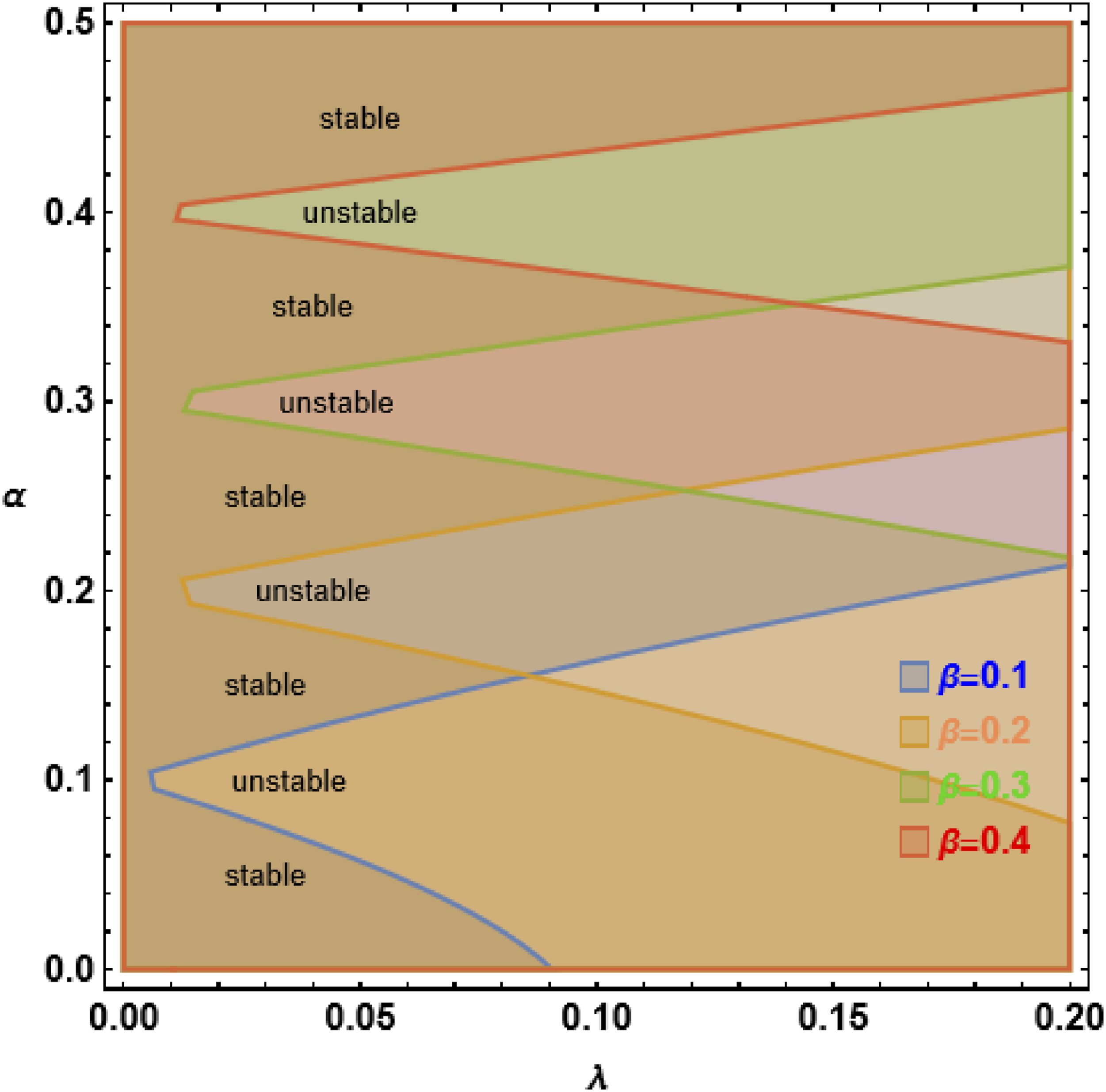 $λ - α)$ for the same system given in Figure 10 except that the parameter p is held fixed at the value p = 1.

The study investigates how the natural frequency ω₁₀ influences stability in a system with fractal resonance, as illustrated in Figure 12. The graph depicts the stability behavior when the natural frequency ω₁₀ is increased, specifically in fractal resonance. Examine how β values of 0.1 and 0.4 affect stability. As ω₁₀ increases, the unstable zone on the stability diagram decreases. This demonstrates that higher natural frequencies stabilize the system under the fractal resonance scenario. The main result is that increasing natural frequencies tends to stabilize the system under fractal resonance conditions, reducing the size of the unstable region.

Figure 12.

Illustrate the influence of the variation in the natural frequency 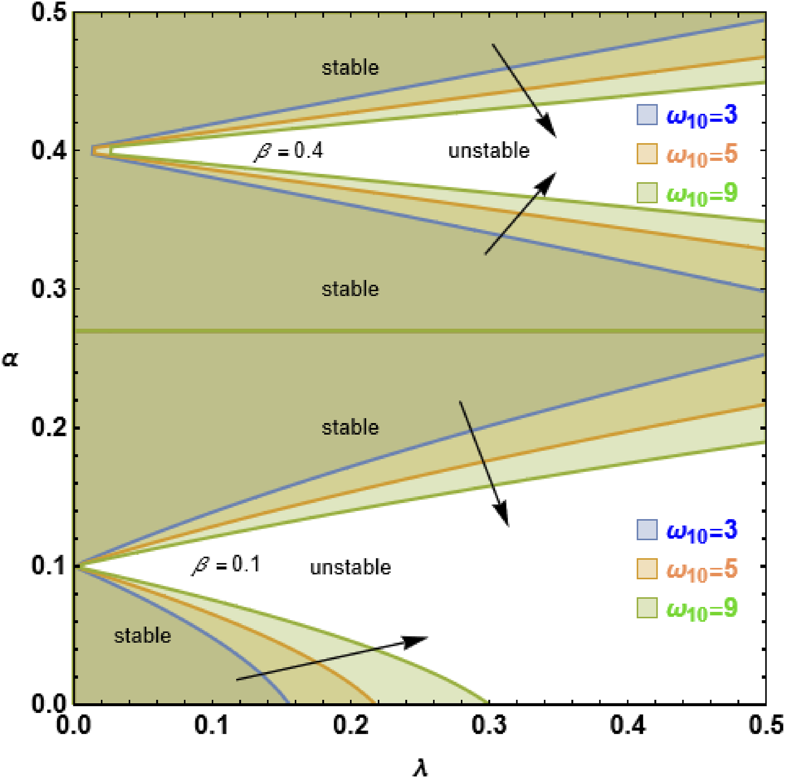$ω$ ₁₀ on the stability behavior in the plane ( $λ - α) .$

The study examines how the parameter σ influences stability behavior in the (λ−α) plane, focusing on the frequency of the external periodic force. The study examines how variations in σ impact stability. The parameter σ is set to fall within predetermined stable intervals of σ ≤ 5.5. Figure 5 illustrates that σ values of ≤5.5 indicate a stable interval. Figure 13 shows the outcomes when σ is within this range. The study discovered that when σ grew from 1 to 5.5, the unstable zone enlarged, indicating a destabilizing effect. Figure 14 demonstrates that increasing σ to σ ≥ 7 decreases the unstable zone, indicating that σ has a stabilizing effect at higher values. Figure 5 indicates an unstable interval of 5.5 < σ < 7. As σ increases, the system’s behavior shifts from stability to destabilization, then back to stability. The study discovered that the parameter σ had two distinct effects on stability. Increasing tiny σ values until σ = 5.5 causes a destabilizing impact, widening the unstable zone. Raising σ ≥ 7 reduces the unstable zone. This study emphasizes the complicated significance of the parameter σ in system stability, revealing that its effect varies according to its value relative to established thresholds.

Figure 13.

Demonstrate how the parameter σ affects stability behavior in the plane (λ−α) by varying σ within the $σ \leq 5.5$ range.

Figure 14.

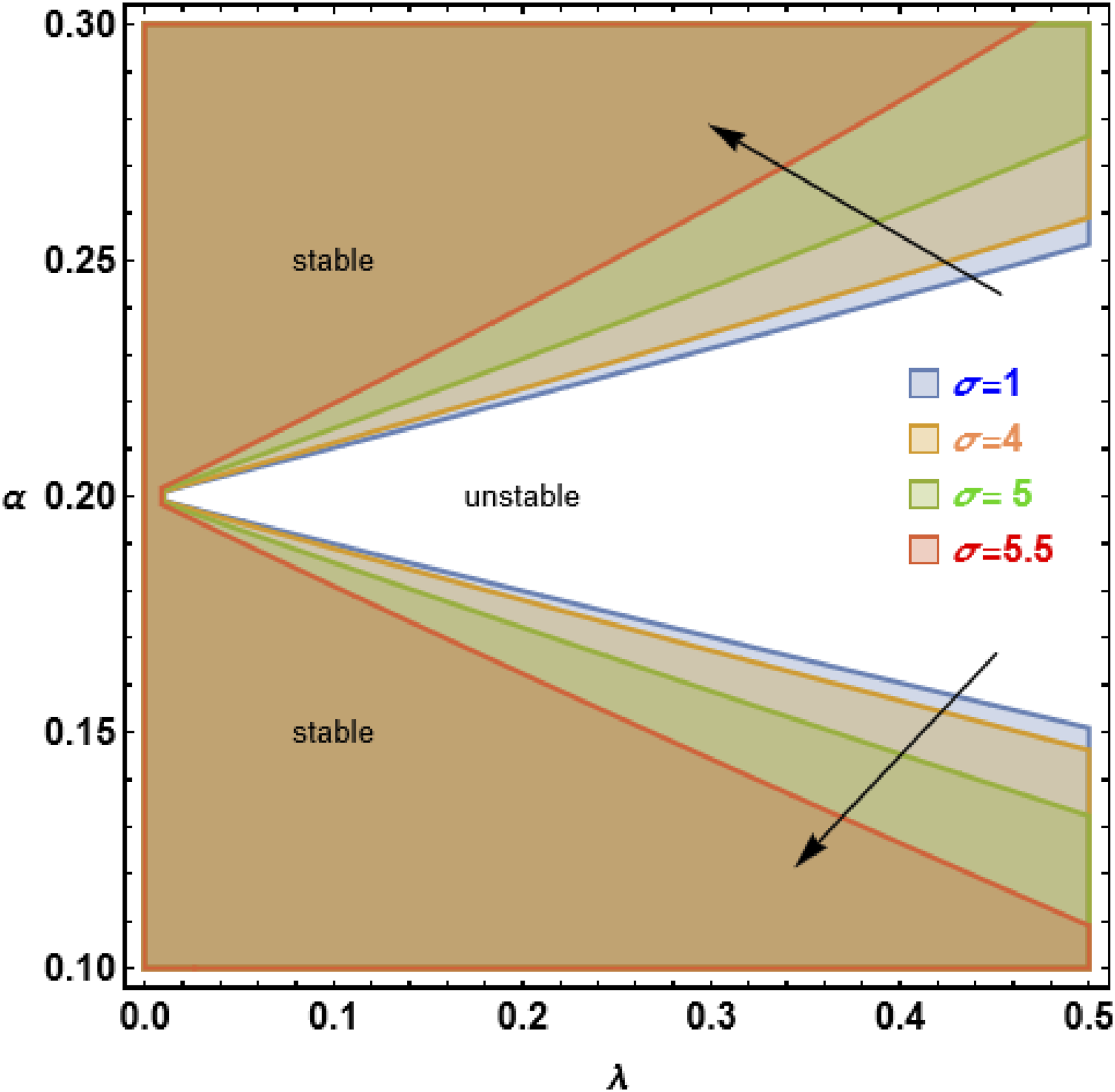
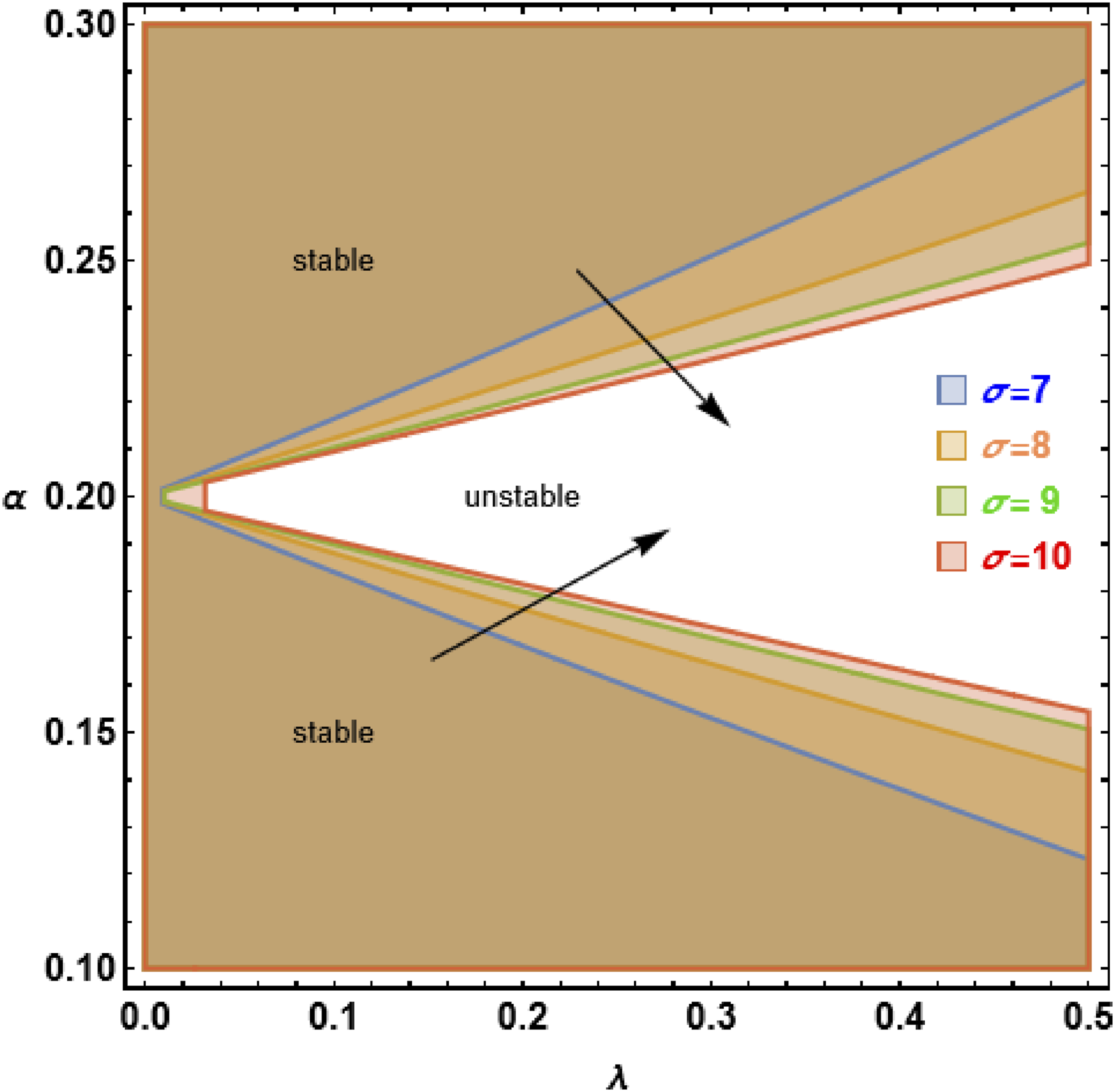
Show how the parameter σ affects stability behavior in the plane (λ−α) with a range of σ $\geq$ 7.

Figure 15 illustrates how fractal resonance, where α approaches β, interacts with harmonic resonance, which is influenced by the frequency of an external periodic force. This interaction is investigated in the (α−σ) plane, with a focus on the impact of varying the periodic force amplitude δ. Figure 15 shows that increasing amplitude δ increases the unstable zone in the stability diagram. This effect is particularly visible in the resonance region, where the parameter σ is very essential. Higher δ results in an increase in the unstable zone, indicating a destabilizing influence. This behavior demonstrates that increasing the amplitude δ worsens instability.

Figure 15.

Represent the stability behavior within the plane (α−σ) with variations in the periodic force amplitude (δ).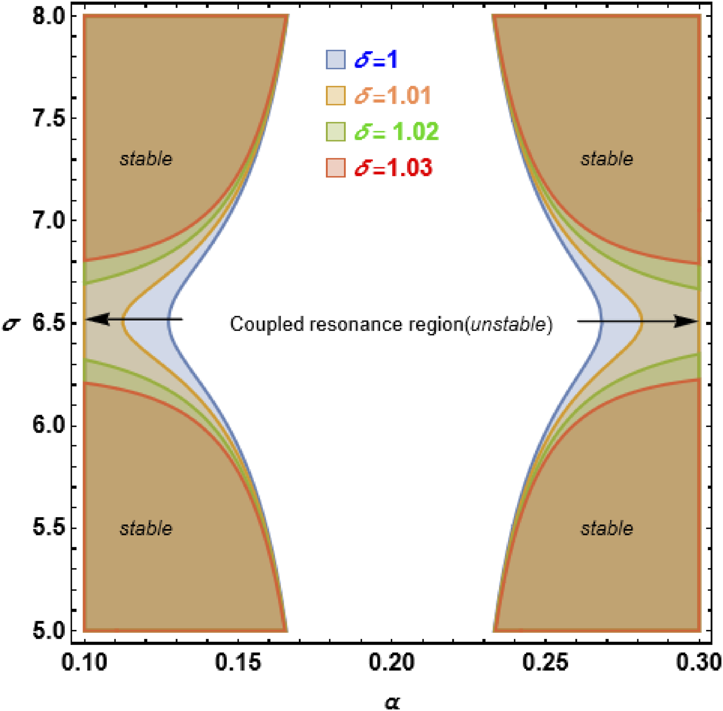

The resonance case of the fractal order $α$ approaches the fractal order. β

Inquire further about the theoretical consequences of having identical fractal orders. Use analytical approaches to investigate how this equality impacts the system’s fundamental features and behaviors. When a specific condition $α = β$ , such as a matching frequency or parameter, is met, solution (58) acts exactly like solution (57) in what is known as the “internal resonance case.” This resonance may produce apparent instability in the system’s dynamics, making it necessary to investigate this particular situation to identify and minimize potential undesired behaviors. To thoroughly investigate this particular case of resonance, the following procedures could be taken:

Incorporate the resonant condition into the equation governing dynamics. For example, resonance occurs when the resonant condition is controlled by a parameter α = β, such that solution (58) equals solution (57). To examine this exceptional example, substitute $α = β = S / 2$ into equation (52), which may take on a new form that directly depicts the dynamics under resonance conditions. This usually results in a simplification or a specific modification of the coefficients or terms:

\frac{d u}{d t^{2 S}} + (\frac{1}{ω_{1} ω_{2}} λ^{2} + 2) \frac{d u}{d t^{S}} + u = 0

(62)

By applying the analytical steps of transformations (34) and (35) to equation (62) to transform into the continuous space with the specified resonant conditions, one can effectively study and comprehend the critical dynamics during resonance, resulting in more robust and reliable system design and operation. So, we have

\ddot{u} + P μ_{0} \dot{u} + P^{2} ϖ_{0}^{2} u = 0

(63)

where

μ_{0} = 2 \cot (\frac{1}{2} π S) + \frac{1}{P^{S} \sin (\frac{1}{2} π S)} (\frac{1}{ω_{1} ω_{2}} λ^{2} + 2)

(64)

ϖ_{0}^{2} = \cot^{2} (\frac{1}{2} π S) + \frac{\cot (\frac{1}{2} π S)}{P^{S} \sin (\frac{1}{2} π S)} (\frac{1}{ω_{1} ω_{2}} λ^{2} + 2) + \frac{1}{P^{2 S} \sin^{2} (\frac{1}{2} π S)}

(65)

Understanding resonance in this work allows for real system design adjustments. To estimate the unknown parameter p in this case, the following relationships are indicated by comparing and with the coefficients of damping and frequency in equation (63):

P (2 \cot (\frac{1}{2} π S) + \frac{1}{P^{S} \sin (\frac{1}{2} π S)} (\frac{1}{ω_{1} ω_{2}} λ^{2} + 2)) = \frac{1}{ω_{1} ω_{2}} λ^{2} + 2

(66)

P^{2} (\cot^{2} (\frac{1}{2} π S) + \frac{\cot (\frac{1}{2} π S)}{P^{S} \sin (\frac{1}{2} π S)} (\frac{1}{ω_{1} ω_{2}} λ^{2} + 2) + \frac{1}{P^{2 S} \sin^{2} (\frac{1}{2} π S)}) = 1

(67)

Solving (66) with (67) yields the following values:

P = (\frac{1}{ω_{1} ω_{2}} λ^{2} + 2) \tan (\frac{1}{2} π S)

(68)

P^{S} = - (\frac{1}{ω_{1} ω_{2}} λ^{2} + 2) \sec (\frac{1}{2} π S)

(69)

Employ (68) and (69) into (63) becomes

\ddot{u} + (\frac{1}{ω_{1} ω_{2}} λ^{2} + 2) \dot{u} + u = 0 .

(70)

The modified form of equation (63) should be tested for stability and resonance behavior. This frequently entails examining the modified frequency equation resulting from the differential equation (70). The frequency (real, complex, positive, or negative) will provide information on the system’s stability behavior under resonant conditions.

In the present example, it is clear that the total frequency of equation (68) has the form

{\tilde{Θ}}^{2} = 1 - \frac{1}{4} {(\frac{1}{ω_{1} ω_{2}} λ^{2} + 2)}^{2}

(71)

The remark about the dynamics of equation (71) emphasizes an important characteristic of system behavior under certain conditions in which the right-hand side of the equation cannot be positive. When the instability becomes obvious as the two fractal orders approach the same value, it indicates a significant transition in the system’s dynamics that must be thoroughly understood and handled.

The convergence of fractal orders to the same value poses a unique challenge to the dynamics of the solutions (57) and (58), especially when this results in negative or zero values on the right-hand side of the frequency equation, indicating intrinsic instability. Understanding and addressing this issue is critical for preserving the appropriate performance and reliability of systems modeled by such equations, particularly in engineering and scientific applications where stability is essential.

Conclusion

This work delves deeply into a dynamic system with two degrees of freedom influenced by a periodic force, distinguishing itself by the use of fractal differential derivatives. By combining complexity with two separate fractal factors, the system’s behavior under multiple dynamic situations is comprehensively examined. The study uses a HELA to convert nonlinear equations into linear equivalents, simplifying the development of analytical solutions. The results show an overdamped response due to fractal factors in damping coefficients. The study also investigates how fractal systems can be transformed into equivalent systems in continuous space. It examines system stability under internal resonance conditions and the reduced harmonic resonance zone. The study highlights the importance of fractal differential derivatives in analyzing advanced dynamic systems and their effectiveness in addressing internal resonance and non-resonance issues. The successful validation of these models underscores the significance of fractal differential derivatives in dynamic system analysis. Future studies can concentrate on forced 2-DOF and 3-DOF oscillatory systems, with fractional adjustments to improve modeling of nonlinear resonance behavior, energy transfer, and stability dynamics. Using several fractional derivative formulations, such as:

1. Use Caputo and Riemann-Liouville Fractional Derivatives to study memory effects and long-term

interactions in oscillatory systems.

2. Use He’s Fractal Derivative to simulate self-similar oscillation patterns and fractal damping in dynamical systems.

3. Atangana-Baleanu Fractional Operators—Investigate non-singular and nonlocal implications on energy dissipation and stability transitions.

4. Apply the fractional complex transformation and spreading residue harmonic balance to transform the fractional oscillator, as described in 36.

Footnotes

ORCID iD

Yusry O El-Dib

Statements and declarations

Author contributions

Contributions of the authors: Every author gave their approval for the manuscript’s published version.

Funding

The authors disclosed receipt of the following financial support for the research, authorship, and/or publication of this article: The authors express their gratitude to Princess Nourah Bint Abdulrahman University Researchers Supporting Project Number (PNURSP2025R17), Princess Nourah Bint Abdulrahman University, Riyadh, Saudi Arabia.

Conflicting interests

The authors declared no potential conflicts of interest with respect to the research, authorship, and/or publication of this article.

References

El-Dib

. Estimated the frequencies of a coupled damped nonlinear oscillator with the non- Perturbative method. J Low Freq Noise Vib Act Control 2023; 42(1): 110–125.

El-Dib

Alyousef

. Successive approximate solutions for nonlinear oscillation and improvement of the solution accuracy with efficient non-perturbative technique. Vibration and Active Control 2023; 42: 1296–1311.

Amer

Ismail

Amer

. Evaluation of the stability of a two degrees-of-freedom dynamical system. J Low Freq Noise Vib Act Control 2023; 42: 1578–1595.

Nayfeh

Mook

. Nonlinear oscillations. Wiley-VCH Verlag GmbH and Co. KGaA, 2004.

Amer

Abdelhfeez

Elbaz

. Modeling and analyzing the motion of a 2DOF dynamical tuned absorber system close to resonance. Arch Appl Mech 2023; 93:785–812.

Liu

Cammarano

Wagg

, et al. $$N-1$$ N - 1 modal interactions of a three-degree-of-freedom system with cubic elastic nonlinearities. Nonlinear Dyn 2016; 83(1–2): 497–511.

Kerschen

Kowtko

Mcfarland

, et al. Theoretical and experimental study of multimodal targeted energy transfer in a system of coupled oscillators. Nonlinear Dyn 2006; 47(1–3): 285–309.

Wang

Zhang

Yao

, et al. Nonlinear characteristics of a multi-degree-of-freedom spur gear system with bending-torsional coupling vibration. Mech Syst Signal Process 2019; 121: 810–827.

Shi

Yang

Wang

. Forced vibration analysis of multi-degree-offreedom nonlinear systems with the extended Galerkin method. Mech Adv Mater Struct 2022; 30: 794–802.

10.

Wang

. The extended Rayleigh-Ritz method for an analysis of nonlinear vibrations. Mech Adv Mater Struct 2021; 29: 3281–3284.

11.

Seth

Kudra

Wasilewski

, et al. Study the bifurcations of a 2DoF mechanical impacting system. Nonlinear Dyn 2024; 112: 1713–1728.

12.

Thygesen

. Stochastic differential equations for science and engineering. 1st ed. Taylor & Francis, 2023.

13.

Moser

Mordinyi

Winkler

, Extending mechatronic objects for automation systems engineering in heterogeneous engineering environments. In: Proceedings of 2012 IEEE 17th international conference on emerging technologies & factory automation (ETFA 2012), Krakow, Poland, 17–21 September 2012. DOI: 10.1109/ETFA.2012.6489664.

14.

Jean-Francois

Pollitt

Bassi

, et al.

Modelling complex systems of heterogeneous agents to better design sustainability transitions policy

2016; 37: 102–115.

15.

Xiao

Huang

, et al. A fractal model for predicting oxygen effective diffusivity of porous media with rough surfaces under dry and wet conditions. Fractals 2021; 29(3): 2150076.

16.

Qian

. A fractal approach to the diffusion process of red ink in a saline water. Therm Sci 2022; 26(3B): 2447–2451.

17.

Zuo

. Effect of sic particles on viscosity of 3-D print paste a fractal rheological model and experimental verification. Therm Sci 2021; 25(3): 2405–2409.

18.

. Fractal variational principle for an optimal control problem. J Low Freq Noise Vib Act Control 2022; 41: 1523–1531.

19.

Wang

. Exact solitary wave solution for fractal shallow water wave model by he’s variational method. Mod Phys Lett B 2022; 36(7): 2150602.

20.

El-Dib

Nada

. Galerkin procedure for resonance analysis of the forced Van der Pol-Duffing-Helmholtz oscillator. J Low Freq Noise Vib Act Control. 2024; 44(1): 461–476. DOI: 10.1177/14613484241275784.

21.

Kou

, et al. Fractal oscillation and its frequency-. Fractals 2021; 29(4): 2150105.

22.

Liang

Gao

Yang

, et al. An analytical model for two-phase relative permeability with Jamin effect in porous media. Fractals 2018; 26(3): 1850037.

23.

Miao

Chen

, et al. A fractal permeability model for porous–fracture media with the transfer of fluids from porous matrix to fracture. Fractals 2019; 27(6): 1950121.

24.

Wang

. A fractal permeability model for real gas in shale reservoirs coupled with Knudsen diffusion and surface diffusion effects. Fractals 2020; 28(1): 2050017.

25.

Sheng

Tian

, et al. A fractal permeability model for shale matrix with multi-scale porous structure. Fractals 2016; 24(1): 1650002.

26.

Wang

Cao

, et al. A fractal model for gas apparent permeability in microfractures of tight/shale reservoirs. Fractals 2017; 25(03): 1750036.

27.

Gao

Cheng

Han

, et al. Fractal analysis of shale gas transport through micropores and microfractures. Fractals 2021; 29(3): 2150068.

28.

Zhang

, et al. A fractal Boussinesq equation for nonlinear transverse vibration of a nanofiber-reinforced concrete pillar. Appl Math Model 2020; 82: 437–448.

29.

. A fractal variational theory for one-dimensional compressible flow in a microgravity space. Fractals 2020; 28(2): 2050024.

30.

Shen

YUE

, et al. Taylor series solution for fractal Bratu-type equation arising in electrospinning process. Fractals 2020; 28(1): 2050011.

31.

Lin

Yao

. Silver ion release from Ag/PET hollow fibers: mathematical model and its application to food packing. J Eng Fiber Fabr 2020; 15: 1558925020935448.

32.

Wang

Yao

Yang

. A fractal derivative model for snow’s thermal insulation property. Therm Sci 2019; 23(4): 2351–2354.

33.

Zuo

Y-T

. Fractal-fractional model for the receptor in a 3D printing system. J Low Freq Noise Vib Act Control 2024; 44: 251–260.

34.

Sun

Zhu

, et al. Numerical analysis of fractional nonlinear vibrations of a restrained cantilever beam with an intermediate lumped mass. Vibration and Active Control 2025; 44: 178–189.

35.

Tian

Ain

Anjum

, et al. Fractal N/MEMS: from pull-ininstability to pull-in stability. Fractals 2021; 29(2): 2150030.

36.

Zheng

Chen

. Numerical analysis of a fractional micro/nanobeam-based micro-electromechanical system. Fractals 2025; 33(1): 2550028.

37.

Caughey

. Equivalent linearization techniques. J Acoust Soc Am 1963; 35(11): 1706–1711.

38.

Wilfred

. On defining equivalent systems for certain ordinary non-linear differential equations. Int J Non Lin Mech 1969; 4: 325–334.

39.

Iwan

. A generalization of the concept of equivalent linearization. Int J Non Lin Mech 1973; 8(3): 279–287.

40.

. Some asymptotic methods for strongly nonlinear equations. Int J Mod Phys B 2006; 20(10): 1141–1199.

41.

. Amplitude–frequency relationship for conservative nonlinear oscillators with odd nonlinearities. Int J Appl Comput Math 2017; 3(2): 1557–1560.

42.

. The simplest approach to nonlinear oscillators. Results Phys 2019; 15: 102546.

43.

J-H

. Frequency formulation for nonlinear oscillators (part 1). Sound Vib 2025; 59(1): 1687.

44.

El-Dib

. The frequency estimation for non-conservative nonlinear oscillation. Z Angew Math Mech 2021; 101(12): e202100187.

45.

El-Dib

. The damping Helmholtz–Rayleigh–Duffing oscillator with the non-perturbative approach. Math Comput Simul 2022; 194: 552–562.

46.

El-Dib

. The simplest approach to solving the cubic nonlinear jerk oscillator with the non-perturbative method. Math Methods Appl Sci 2022; 45(9): 5165–5183.

47.

J-H

. The simpler, the better: analytical methods for nonlinear oscillators and fractional oscillators. J Low Freq Noise Vib Act Control 2019; 38: 1252–1260.

48.

El-Dib

. Insightful and comprehensive formularization of frequency–amplitude formula for strong or singular nonlinear os cillators. J Low Freq Noise Vib Act Control 2023; 42(1): 89–109.

49.

El-Dib

. Insights into fractal space features in nonlinear electrohydrodynamic Rayleigh–Taylor instability of viscous fluids. Phys Fluids 2024; 36: 122127.

50.

El-Dib

. An innovative efficient approach to solving damped Mathieu–Duffing equation with the non-perturbative technique. Commun Nonlinear Sci Numer Simul 2024; 128: 107590.

51.

El-Dib

. The masking technique for forced nonlinear oscillator stability behavior analysis using the non-perturbative approach. Vibration and Active Control 2024; 43: 1481–1497.

52.

El-Dib

. Stability analysis of a time-delayed Van der Pol–Helmholtz–Duffing oscillator in fractal space with a non-perturbative approach. Commun Theor Phys 2024; 76: 045003.

53.

Yang

, et al. Pull-down instability of the quadratic nonlinear oscillators. FU Mech Eng 2023; 21: 191.

54.

El-Dib

Alyousef

. A new perspective on the dynamic forced 2-DOF system with the non-perturbative approach. Int J Non Lin Mech 2023; 157: 104539.

55.

El-Dib

. A review of the frequency-amplitude formula for nonlinear oscillators and its advancements. J Low Freq Noise Vib Act Control 2024; 43: 1032–1064.

56.

El-Dib

Elgazery

. A novel pattern in a class of fractal models with the non-perturbative approach. Chaos Solitons Fractals. 2022; 164: 112694.

57.

. A tutorial review on fractal spacetime and fractional calculus. Int J Theor Phys 2014; 53: 3698–3718.

58.

. Fractal calculus and its geometrical explanation. Results Phys 2018; 10: 272–276.

59.

El-Dib

. A tutorial introduction to the two-scale fractal calculus and its application to the fractal zhiber-shabat oscillator. Fractals. 2021; 29(8): 2150268. DOI: 10.1142/S0218348X21502686.

Modified Lindstedt-Poincare transformation for fractal resonance approach in vibration 2-DOF heterogeneous system

Abstract

Keywords

Introduction

Dynamical model and immediate frequencies and solutions identification

The non-resonance analysis

Numerical validation and discussion for the non-internal resonance case

Common frequency approach (internal resonance case)

Analysis of stability and behavior in the internal resonance case

Numerical illustration and stability discussion

The resonance case of the fractal order α approaches the fractal order. β

Conclusion

Footnotes

ORCID iD

Statements and declarations

Author contributions

Funding

Conflicting interests

References

The resonance case of the fractal order $α$ approaches the fractal order. β