Sage Journals: Discover world-class research

Abstract

A modified harmonic balance method (MHBM) has been extended for solving strongly nonlinear damped forced oscillators with quadratic-biquadratic nonlinearities. Depending on the parameter values and initial conditions, its behavior is quite complex. The proposed method allows us to expand some Fourier coefficients in a power series, which helps to provide analytical solutions. Traditional perturbation methods (e.g., averaging, Krylov-Bogoliubov-Mitropolskii (KBM), and multiple time scale) and the classical harmonic balance method are often inadequate for obtaining similar approximate solutions. The solutions obtained by the proposed method nicely coincide with corresponding numerical solutions.

Keywords

HBM MHBM Perturbation method homotopy perturbation method nonlinear oscillators and exciting periodic force 34E05 34E10 34M10

Introduction

Most physical and engineering problems emerge in nonlinear differential equations (NDEs), such as mechanical oscillations, electrical circuits, chemical reactions, biological systems, plasma physics, and solid mechanics. The equation could represent the motion of a damped nonlinear mechanical oscillator subject to an external periodic force. The equation could be used to model certain nonlinear electrical circuits subjected to an external sinusoidal voltage source. This equation might be applicable to describe the concentration of a reactant in a reaction system subjected to an external oscillating influence. Nonlinear differential equations are also commonly used to model biological systems, such as population dynamics or biochemical reactions, where external periodic influences play a significant role. Therefore, it is evident that the capability to analyze, solve, and comprehend differential equations is of fundamental importance for applied mathematicians, physicists, and engineers. The nature and behavior of the systems are known by these solutions. Rarely do appropriate solutions arise for these nonlinear oscillators. As a result, numerous researchers and scientists have directed their focus toward the development of both numerical techniques and analytical methods. Numerical techniques involve procedures to determine true values at specific discrete points, achieved through incremental improvement. Successful application of numerical techniques relies on having suitable initial guess values. While these techniques are generally straightforward, they can sometimes demand significant computational effort and appropriate approximate values to yield desired results. Additionally, the numerical techniques fail to capture an overall picture of nonlinear dynamical systems. Moreover, obtaining amplitude and phase in nonlinear dynamical system using numerical techniques proves to be a laborious task.

On the other hand, approximation methods have garnered significant interest among scientists, physicists, engineers, and applied mathematicians due to their analytical expressions and suitability for parametric study. There are many methods to deal with the nonlinear differential equations with nonlinear stiffness and damping, such as the averaging method,^2–4 KBM method,^5,6 and multi-scale method^2–4 and so on.

Numerous methods of approximation investigated to tackle nonlinear oscillators, encompassing the perturbation method,^1–11 homotopy analysis technique,^12,13 homotopy perturbation technique,^14–16 variational iteration technique,^17,18 harmonic balance method (HBM),^19–24 modified multi-level residue harmonic balance method,^25–27 and modified harmonic balance method (HBM),^29–32 among others. Perturbation methods^1–11 find widespread application for weakly nonlinear oscillators. Jones⁹ made advancements to the classical perturbation technique to enhance its scope and precision for both large and small parameters. Cheung et al.¹⁰ modified the Lindstedt-Poincare technique based on Jones’⁹ ideas, while Alam et al.¹¹ exhibited a modified Lindstedt-Poincare technique to control oscillators with strong nonlinearities.

The HBM and MHBM are also valuable methods for computing periodic solutions of nonlinear oscillators. These methods involve selecting a truncated Fourier series as a solution. In classical HBM, a system of nonlinear algebraic equations is solved numerically to determine the values of the unknown coefficients. Several authors revised this method.^19–24 For instance, Rahman et al.²⁰ exerted the HBM to solve the Van der Pol equation, and Wagner and Lentz²¹ explored it for determining solutions of nonlinear oscillators. Several authors^22–33 developed HBM and MHBM for tackling nonlinear physical systems. Furthermore, Uddin and Sattar³⁴ developed a technique for handling strongly damped nonlinear biological systems without periodic excitation. It is interesting to point out that the MHBM has not been explored yet for solving a damped nonlinear forced oscillator with quadratic-biquadratic nonlinearities. In this article, this gap has been filled.

The method

We hypothesize a nonlinear forced oscillator with damping and quadratic-biquadratic nonlinearities^29–34

\ddot{x} + μ \dot{x} + x + ε f (x) = p c o s (ω t),

(1)where

x

is the displacement of the system from its equilibrium position,

μ

is the coefficient of damping and

f (x)

is a generalized function for quadratic-biquadratic nonlinearities,

0 < ε \leq 1

is a parameter which measured the strength of nonlinearities,

p

and

ω

represent the amplitude and the angular frequency of the periodic driving force, respectively,

t

is time and over dots represent the time derivatives of the position

x

The solution of Eq. (1) is considered to be

x (t) = a_{0} + a_{1} \cos (ω t) + b_{1} \sin (ω t) + a_{2} \cos (2 ω t) + b_{2} \sin (2 ω t) + \dots .

(2)where

a_{0}, a_{1}, b_{1}, a_{2}, b_{2} \dots

are to be destined. Inserting Eq. (2) into Eq. (1) and stretching

f (x)

in a Fourier series and collecting the like harmonics, we attain

f (a_{0}, a_{1}, b_{1}, a_{2}, b_{2}, \dots) = 0

(3a)

(1 - ω^{2}) a_{1} + μ ω b_{1} + ε A_{1} (a_{0}, a_{1}, b_{1}, a_{2}, b_{2}, \dots) = p

(3b)

(1 - ω^{2}) b_{1} - μ ω a_{1} + ε B_{1} (a_{0}, a_{1}, b_{1}, a_{2}, b_{2}, \dots) = 0

(3c)

(1 - 4 ω^{2}) a_{2} + 2 μ ω b_{2} + ε A_{2} (a_{0}, a_{1}, b_{1}, a_{2}, b_{2}, \dots) = 0

(3d)

(1 - 4 ω^{2}) b_{2} - 2 μ ω a_{2} + ε B_{2} (a_{0}, a_{1}, b_{1}, a_{2}, b_{2}, \dots) = 0 .

(3e)

According to the classical HBM, five simultaneous nonlinear Eqs. (3a)-(3e) are required to solve by a numerical method to determine the unknown coefficients. It is difficult task. Also, it requires a heavy computational effort and proper numerical initial guess values to obtain the desired solutions. But the present approach overcomes this issue. In the proposed method, only one equation has been solved numerically and the rest of four simultaneous nonlinear equations have been solved analytically. It makes it easier to simplify and allow to ignoring some terms by taking the linear terms of $a_{2}$ and $b_{2}$ (Please see Appendix-A). It makes easier to solve four simultaneous nonlinear equations analytically. Deducting $ω^{2}$ from Eqs. (3c)-(3e) employing Eq. (3b), and discarding the terms with insignificant responses, then Eqs. (3b)-(3e) turn out the form

ω^{2} = 1 + μ ω b_{1} / a_{1} + ϵ A_{1} (a_{0}, a_{1}, b_{1}, a_{2}, b_{2}, \dots) - p / a_{1}

(4a)

- 4 μ ω a_{1} + 4 p b_{1} / a_{1} - ϵ A_{1} (a_{0}, a_{1}, b_{1}, a_{2}, b_{2}, \dots) + ϵ B_{1} (a_{0}, a_{1}, b_{1}, a_{2}, b_{2}, \dots) = 0

(4b)

\frac{μ ω (- 16 a_{2} b_{1} + 8 a_{1} b_{2})}{a_{1}} + \frac{16 p a_{2} - 12 a_{1} a_{2}}{a_{1}} - ϵ A_{2} (a_{0}, a_{1}, b_{1}, a_{2}, b_{2}, \dots) + ϵ B_{2} (a_{0}, a_{1}, b_{1}, a_{2}, b_{2}, \dots) = 0

(4c)

\frac{μ ω (- 8 a_{1} a_{2} - 16 b_{1} b_{2})}{a_{1}} + \frac{16 p b_{2} - 12 a_{1} b_{2}}{a_{1}} - ϵ A_{1} (a_{0}, a_{1}, b_{1}, a_{2}, b_{2}, \dots) + ϵ B_{2} (a_{0}, a_{1}, b_{1}, a_{2}, b_{2}, \dots) = 0 .

(4d)

Employing Eq. (4b), discarding $ω$ from Eqs. (4c) and (4d) and considering only the first-order terms and ignoring higher-order ones of $a_{2}, b_{2}$ , a set of linear system of equations of $a_{2}, b_{2}$ are achieved. After simplifying, $a_{2}, b_{2}$ are acquired in terms of $a_{0}, a_{1}, b_{1}$ . Finally, inserting $a_{2}, b_{2}$ in Eq. (4b) and $b_{1}$ is stretching in a power series of $λ (μ, ω, p)$ , we acquire

b_{1} = l_{0} λ + l_{1} λ^{3} + l_{2} λ^{5} + \dots,

(5)where

l_{0}, l_{1}, l_{2}, \dots

are functions of

a_{1}

and

λ

is small parameter. Inserting

a_{2}, b_{2}

and

b_{1}

in Eq. (3a) and

a_{0}

is stretching in a power series of

δ (ε, a_{1})

, we acquire

a_{0} = m_{0} + m_{1} δ + m_{2} δ^{2} + \dots,

(6)where

m_{0}, m_{1}, m_{2}, \dots

are function of

a_{1}

and

b_{1}

and

δ

is small parameter. Now inserting

a_{0}, b_{1} a_{2}

and

b_{2}

in Eq. (3b),

a_{1}

is obtained. Systematically,

a_{0}, b_{1}, a_{2}

and

b_{2}

are achieved.

Example

Let’s examine a generalized nonlinear damped oscillator^29–32,34 with periodic driving force and quadratic-biquadratic nonlinearities of the form

\ddot{x} + μ \dot{x} + x + ε (x^{2} + x^{4}) = p \cos (ω t) .

(7)

The solution of Eq. (7) is assumed to be

x (t) = a_{0} + a_{1} \cos (ω t) + b_{1} \sin (ω t) + a_{2} \cos (2 ω t) + b_{2} \sin (2 ω t) .

(8)

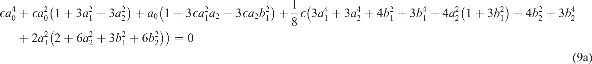
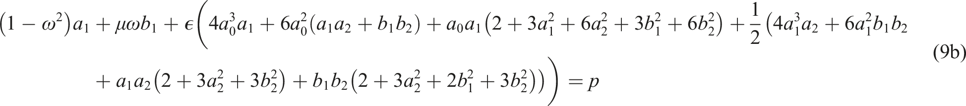
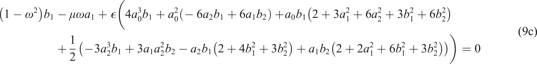
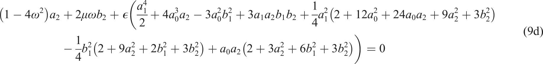
The values of the undetermined coefficients $a_{0}, a_{1}, b_{1}, a_{2},$ and $b_{2}$ are required to find to obtain the required results. Inserting Eq. (8) into Eq. (7), collecting the like harmonics, and discarding the terms with insignificant responses, we achieve

ϵ a_{0}^{4} + ϵ a_{0}^{2} (1 + 3 a_{1}^{2} + 3 a_{2}^{2}) + a_{0} (1 + 3 ϵ a_{1}^{2} a_{2} - 3 ϵ a_{2} b_{1}^{2}) + \frac{1}{8} ϵ (3 a_{1}^{4} + 3 a_{2}^{4} + 4 b_{1}^{2} + 3 b_{1}^{4} + 4 a_{2}^{2} (1 + 3 b_{1}^{2}) + 4 b_{2}^{2} + 3 b_{2}^{4} + 2 a_{1}^{2} (2 + 6 a_{2}^{2} + 3 b_{1}^{2} + 6 b_{2}^{2})) = 0

(9a)

(1 - ω^{2}) a_{1} + μ ω b_{1} + ϵ (4 a_{0}^{3} a_{1} + 6 a_{0}^{2} (a_{1} a_{2} + b_{1} b_{2}) + a_{0} a_{1} (2 + 3 a_{1}^{2} + 6 a_{2}^{2} + 3 b_{1}^{2} + 6 b_{2}^{2}) + \frac{1}{2} (4 a_{1}^{3} a_{2} + 6 a_{1}^{2} b_{1} b_{2} + a_{1} a_{2} (2 + 3 a_{2}^{2} + 3 b_{2}^{2}) + b_{1} b_{2} (2 + 3 a_{2}^{2} + 2 b_{1}^{2} + 3 b_{2}^{2}))) = p

(9b)

(1 - ω^{2}) b_{1} - μ ω a_{1} + ϵ (4 a_{0}^{3} b_{1} + a_{0}^{2} (- 6 a_{2} b_{1} + 6 a_{1} b_{2}) + a_{0} b_{1} (2 + 3 a_{1}^{2} + 6 a_{2}^{2} + 3 b_{1}^{2} + 6 b_{2}^{2}) + \frac{1}{2} (- 3 a_{2}^{3} b_{1} + 3 a_{1} a_{2}^{2} b_{2} - a_{2} b_{1} (2 + 4 b_{1}^{2} + 3 b_{2}^{2}) + a_{1} b_{2} (2 + 2 a_{1}^{2} + 6 b_{1}^{2} + 3 b_{2}^{2}))) = 0

(9c)

(1 - 4 ω^{2}) a_{2} + 2 μ ω b_{2} + ϵ (\frac{a_{1}^{4}}{2} + 4 a_{0}^{3} a_{2} - 3 a_{0}^{2} b_{1}^{2} + 3 a_{1} a_{2} b_{1} b_{2} + \frac{1}{4} a_{1}^{2} (2 + 12 a_{0}^{2} + 24 a_{0} a_{2} + 9 a_{2}^{2} + 3 b_{2}^{2}) - \frac{1}{4} b_{1}^{2} (2 + 9 a_{2}^{2} + 2 b_{1}^{2} + 3 b_{2}^{2}) + a_{0} a_{2} (2 + 3 a_{2}^{2} + 6 b_{1}^{2} + 3 b_{2}^{2})) = 0

(9d)

(1 - 4 ω^{2}) b_{2} - 2 μ ω a_{2} + \frac{ϵ}{2} (2 a_{1}^{3} b_{1} + 3 a_{1}^{2} (4 a_{0} + a_{2}) b_{2} + a_{1} b_{1} (2 + 12 a_{0}^{2} + 3 a_{2}^{2} + 2 b_{1}^{2} + 9 b_{2}^{2}) + b_{2} (8 a_{0}^{3} - 3 a_{2} b_{1}^{2} + 2 a_{0} (2 + 3 a_{2}^{2} + 6 b_{1}^{2} + 3 b_{2}^{2}))) = 0

(9e)

Deducting $ω^{2}$ from Eqs. (9c)-(9e) employing Eq. (9b), and discarding the terms with insignificant responses, then Eqs. (9c)-(9e) turn out the form

4 p b_{1} - 4 (a_{1}^{2} + b_{1}^{2}) μ ω + 4 ϵ (1 + 6 a_{0}^{2} + a_{1}^{2} + b_{1}^{2}) (- 2 a_{1} a_{2} b_{1} + a_{1}^{2} b_{2} - b_{1}^{2} b_{2}) = 0 .

(10a)

μ ω (- 16 a_{2} b_{1} + 8 a_{1} b_{2}) - 12 a_{1} a_{2} + 16 p a_{2} - 2 ϵ a_{1} (- a_{1}^{4} + 24 a_{0}^{3} a_{2} + a_{1}^{2} (- 1 - 6 a_{0}^{2} + 12 a_{0} a_{2}) + b_{1}^{2} + 6 a_{0}^{2} b_{1}^{2} + b_{1}^{4} + 12 a_{0} a_{2} (1 + b_{1}^{2})) = 0 .

(10b)

16 p b_{2} - 12 a_{1} b_{2} - μ ω (- 8 a_{1} a_{2} - 16 b_{1} b_{2}) + ϵ a_{1} (4 a_{1}^{3} b_{1} + a_{1} b_{1} (1 + 24 a_{0}^{2} + 4 b_{1}^{2}) - 24 a_{0} a_{1}^{2} b_{1}^{2} - 24 a_{0} (1 + 2 a_{0}^{2} + b_{1}^{2}) b_{2}) = 0 .

(10c)

By employing Eq. (10a), deducting ω from Eqs. (10b) and (10c), and picking up the linear components of $a_{2}$ , $b_{2}$ and discarding the terms with insignificant repercussions, we achieve

64 p a_{1}^{2} a_{2} - 48 a_{1}^{3} a_{2} - 48 a_{1} a_{2} b_{1}^{2} + 8 ϵ a_{1} (a_{1}^{2} + b_{1}^{2}) (a_{1}^{4} - 24 a_{0}^{3} a_{2} + a_{1}^{2} (1 + 6 a_{0}^{2} - 12 a_{0} a_{2}) - 6 a_{0}^{2} b_{1}^{2} - 12 a_{0} a_{2} (1 + b_{1}^{2}) - b_{1}^{2} (1 + b_{1}^{2})) = 0 .

(11a)

- 16 a_{1} (- 4 p a_{1} + 3 a_{1}^{2} + 3 b_{1}^{2}) b_{2} + 16 ϵ a_{1} (a_{1}^{2} + b_{1}^{2}) (a_{1}^{3} b_{1} + a_{1} b_{1} (1 + 6 a_{0}^{2} + b_{1}^{2}) - 6 a_{0} a_{1}^{2} b_{2} - 6 a_{0} (1 + 2 a_{0}^{2} + b_{1}^{2}) b_{2}) = 0 .

(11b)

Simplifying Eq. (11a) and Eq. (11b), $a_{2}$ and $b_{2}$ are obtained as follows

a_{2} = \frac{- ϵ (1 + 6 a_{0}^{2} + a_{1}^{2} + b_{1}^{2}) (a_{1}^{4} - b_{1}^{4})}{2 (4 p a_{1} - 3 a_{1}^{2} - 3 b_{1}^{2} - 6 ϵ a_{0} (a_{1}^{2} + b_{1}^{2}) (1 + 2 a_{0}^{2} + a_{1}^{2} + b_{1}^{2}))} .

(12a)

b_{2} = \frac{- ϵ a_{1} b_{1} (a_{1}^{2} + b_{1}^{2}) (1 + 6 a_{0}^{2} + a_{1}^{2} + b_{1}^{2})}{(4 p a_{1} - 3 a_{1}^{2} - 3 b_{1}^{2} - 6 ϵ a_{0} (a_{1}^{2} + b_{1}^{2}) (1 + 2 a_{0}^{2} + a_{1}^{2} + b_{1}^{2}))} .

(12b)

Inserting $a_{2}$ and $b_{2}$ in Eq. (10a), and then $b_{1}$ is stretching in a power series of $λ$ , we acquire

b_{1} = a_{1}^{2} λ + a_{1}^{4} λ^{3} + 2 a_{1}^{6} λ^{5},

(13a)where

λ = \frac{μ ω}{p} .

(13b)

Again inserting $a_{2}, b_{2}$ and $b_{1}$ in Eq. (9a) and $a_{0}$ is stretching in a power series of $δ (ε, a_{1})$ , we acquire

a_{0} = m_{0} + m_{1} δ + m_{2} δ^{2} + \dots,

(14a)where

m_{0} = - \frac{ϵ}{2} (a_{1}^{2} + b_{1}^{2}), m_{1} = - \frac{ϵ^{2}}{64} {(4 a_{1}^{2} + 3 a_{1}^{4} + 4 b_{1}^{2} + 6 a_{1}^{2} b_{1}^{2} + 3 b_{1}^{4})}^{2},

m_{2} = - \frac{ϵ^{3}}{256} {(4 a_{1}^{2} + 3 a_{1}^{4} + 4 b_{1}^{2} + 6 a_{1}^{2} b_{1}^{2} + 3 b_{1}^{4})}^{3}, δ = ϵ (1 + 3 a_{1}^{2}) .

(14b)Finally, inserting

a_{0}

a_{2}

b_{1}

and

b_{2}

into Eq. (9b) and solving,

a_{1}

is obtained. Systematically,

a_{0}, b_{1}, a_{2}

and

b_{2}

are achieved.

Example

Let’s examine a nonlinear damped oscillator subjected to an external periodic force^29–32 with quadratic^4,34 nonlinearity of the form

\ddot{x} + μ \dot{x} + x + ε x^{2} = p \cos (ω t) .

(15)

Inserting Eq. (8) into Eq. (15), collecting the like harmonics, and discarding the terms with insignificant responses, we achieve

a_{0} + ϵ a_{0}^{2} + \frac{1}{2} ϵ (a_{1}^{2} + a_{2}^{2} + b_{1}^{2} + b_{2}^{2}) = 0 .

(16a)

a_{1} (1 - ω^{2}) + ϵ a_{1} (2 a_{0} + a_{2}) + b_{1} (μ ω + ϵ b_{2}) = p .

(16b)

(1 - ω^{2}) b_{1} - μ ω a_{1} + ϵ (2 a_{0} b_{1} - a_{2} b_{1} + a_{1} b_{2}) = 0 .

(16c)

(1 - 4 ω^{2}) a_{2} + \frac{ϵ}{2} (a_{1}^{2} + 4 a_{0} a_{2} - b_{1}^{2}) + 2 μ ω b_{2} = 0 .

(16d)

(1 - 4 ω^{2}) b_{2} - 2 μ ω a_{2} + ϵ (a_{1} b_{1} + 2 a_{0} b_{2}) = 0 .

(16e)

Deducting $ω^{2}$ from Eqs. (16c)-(16e) employing Eq. (16b), and discarding the terms with insignificant responses, then Eqs. (16c)-(16e) turn out the form

p b_{1} - μ ω (b_{1}^{2} + a_{1}^{2}) - ϵ (2 a_{1} a_{2} b_{1} - a_{1}^{2} b_{2} + b_{1}^{2} b_{2}) = 0 .

(17a)

16 p a_{2} - 12 a_{1} a_{2} + μ ω (- 16 a_{2} b_{1} + 8 a_{1} b_{2}) + 2 ϵ (a_{1}^{3} - 12 a_{0} a_{1} a_{2} - 8 a_{1} a_{2}^{2} - a_{1} b_{1}^{2} - 8 a_{2} b_{1} b_{2}) = 0 .

(17b)

16 p b_{2} - 12 a_{1} b_{2} + μ ω (- 16 b_{1} b_{2} - 8 a_{1} a_{2}) + 4 ϵ (a_{1}^{2} b_{1} - 6 a_{0} a_{1} b_{2} - 4 a_{1} a_{2} b_{2} - 4 b_{1} b_{2}^{2}) = 0 .

(17c)

By employing Eq. (17a), deducting ω from Eqs. (17b) and (17c), and picking up the linear components of $a_{2}$ , $b_{2}$ and discarding the components with insignificant effects, we achieve

16 a_{2} (4 p a_{1} - 3 a_{1}^{2} - 3 b_{1}^{2}) + 8 ϵ (a_{1}^{2} - 12 a_{0} a_{2} - b_{1}^{2}) (a_{1}^{2} + b_{1}^{2}) = 0

(18a)

- 16 a_{1} (- 4 p a_{1} + 3 a_{1}^{2} + 3 b_{1}^{2}) b_{2} + 16 ϵ a_{1} (a_{1}^{3} b_{1} + a_{1} b_{1}^{3} - 6 a_{0} a_{1}^{2} b_{2} + 6 (- a_{0} + a_{2}) b_{1}^{2} b_{2}) = 0 .

(18b)

Simplifying Eqs. (18a) and (18b), we attain

a_{2} = - \frac{- ϵ a_{1}^{4} + ϵ b_{1}^{4}}{2 a_{1} (- 4 p + 3 a_{1} + 6 ϵ a_{0} a_{1})} .

(19a)

b_{2} = \frac{- ϵ a_{1}^{2} b_{1} - ϵ b_{1}^{3}}{4 p - 3 a_{1} - 6 ϵ a_{0} a_{1}} .

(19b)

Inserting $a_{2}$ and $b_{2}$ in Eq. (17a), and then $b_{1}$ is stretching in a power series of $λ$ , we acquire

b_{1} = a_{1}^{2} λ + a_{1}^{4} λ^{3} + 2 a_{1}^{6} λ^{5} .

(20a)

λ = \frac{μ ω}{p} .

(20b)

Again inserting $a_{2}, b_{2}$ and $b_{1}$ in Eq. (16a) and $a_{0}$ is stretching in a power series of $δ (ε)$ , we acquire

a_{0} = m_{0} + m_{1} δ^{2} + m_{2} δ^{4} + m_{3} δ^{6} + \dots,

(21a)where

m_{0} = \frac{- ϵ a_{1}^{2}}{4} (2 + ϵ^{2} a_{1}^{2} + ϵ^{4} a_{1}^{4}); m_{1} = \frac{- ϵ a_{1}^{4}}{4} (2 + 2 ϵ^{2} a_{1}^{2} + 3 ϵ^{4} a_{1}^{4})

m_{2} = \frac{- ϵ a_{1}^{6}}{4} (4 + 5 ϵ^{2} a_{1}^{2} + 9 ϵ^{4} a_{1}^{4}), m_{3} = \frac{- ϵ a_{1}^{8}}{4} (5 + 7 ϵ^{2} a_{1}^{2} + 14 ϵ^{4} a_{1}^{4}) .

(21b)

Finally, inserting $a_{0}$ , $a_{2}$ , $b_{1}$ and $b_{2}$ into Eq. (16b) and solving, $a_{1}$ is obtained. Systematically, $a_{0}, b_{1}, a_{2}$ and $b_{2}$ are achieved.

Example

Let’s examine a nonlinear damped oscillator subjected to an external periodic force^29–32 with biquadratic⁴ nonlinearity of the form

\ddot{x} + μ \dot{x} + x + ε x^{4} = p \cos (ω t) .

(21)

Substituting Eq. (8) into Eq. (21), collecting the like harmonics, and discarding the terms with insignificant responses, we achieve

ϵ a_{0}^{4} + 3 ϵ a_{0}^{2} (a_{1}^{2} + b_{1}^{2}) + \frac{3}{8} ϵ {(a_{1}^{2} + b_{1}^{2})}^{2} + a_{0} (1 + 3 ϵ a_{1}^{2} a_{2} - 3 ϵ a_{2} b_{1}^{2} + 6 ϵ a_{1} b_{1} b_{2}) = 0 .

(22a)

(1 - ω^{2}) a_{1} + μ ω b_{1} + ϵ (4 a_{0}^{3} a_{1} + 2 a_{1}^{3} a_{2} + 3 a_{0} a_{1} (a_{1}^{2} + b_{1}^{2}) + 3 a_{1}^{2} b_{1} b_{2} + b_{1}^{3} b_{2} + 6 a_{0}^{2} (a_{1} a_{2} + b_{1} b_{2})) = p .

(22b)

(1 - ω^{2}) b_{1} - μ ω a_{1} + ϵ (4 a_{0}^{3} b_{1} - 2 a_{2} b_{1}^{3} + 3 a_{0} b_{1} (a_{1}^{2} + b_{1}^{2}) + a_{1} (a_{1}^{2} + 3 b_{1}^{2}) b_{2} + a_{0}^{2} (- 6 a_{2} b_{1} + 6 a_{1} b_{2})) = 0 .

(22c)

(1 - 4 ω^{2}) a_{2} + 2 μ ω b_{2} + \frac{1}{2} ϵ (a_{1}^{4} + 8 a_{0}^{3} a_{2} - b_{1}^{4} + 6 a_{0}^{2} (a_{1}^{2} - b_{1}^{2}) + 12 a_{0} a_{2} (a_{1}^{2} + b_{1}^{2})) = 0 .

(22d)

(1 - 4 ω^{2}) b_{2} - 2 μ ω a_{2} + ϵ (6 a_{0}^{2} a_{1} b_{1} + a_{1} b_{1} (a_{1}^{2} + b_{1}^{2}) + 4 a_{0}^{3} b_{2} + 6 a_{0} b_{2} (a_{1}^{2} + b_{1}^{2})) = 0 .

(22e)

Deducting $ω^{2}$ from Eqs. (22c)-(22e) employing Eq. (22b), and discarding the terms with insignificant responses, then Eqs. (22c)-(22e) lead to the form

4 p b_{1} - 4 μ ω (a_{1}^{2} + b_{1}^{2}) + 4 ϵ (6 a_{0}^{2} + a_{1}^{2} + b_{1}^{2}) (- 2 a_{1} a_{2} b_{1} + a_{1}^{2} b_{2} - b_{1}^{2} b_{2}) = 0

(23a)

8 μ ω (a_{1} b_{2} - 2 a_{2} b_{1}) + 16 p a_{2} - 12 a_{1} a_{2} - 2 ϵ a_{1} (- a_{1}^{4} + 24 a_{0}^{3} a_{2} + b_{1}^{4} - 6 a_{0}^{2} (a_{1}^{2} - b_{1}^{2}) + 12 a_{0} a_{2} (a_{1}^{2} + b_{1}^{2})) = 0 .

(23b)

16 p b_{2} - 12 a_{1} b_{2} - 8 μ ω (a_{1} a_{2} - 2 b_{2} b_{1}) + 4 ϵ a_{1} (6 a_{0}^{2} a_{1} b_{1} + a_{1} b_{1} (a_{1}^{2} + b_{1}^{2}) - 12 a_{0}^{3} b_{2} - 6 a_{0} (a_{1}^{2} + b_{1}^{2}) b_{2}) = 0 .

(23c)

By employing Eq. (23a), deducting ω from Eqs. (23b) and (23c), and picking up the linear components of $a_{2}$ , $b_{2}$ and discarding the terms with insignificant repercussions, we achieve

- 16 a_{1} a_{2} (- 4 p a_{1} + 3 a_{1}^{2} + 3 b_{1}^{2}) - 8 ϵ a_{1} (a_{1}^{2} + b_{1}^{2}) (- a_{1}^{4} + 24 a_{0}^{3} a_{2} + b_{1}^{4} - 6 a_{0}^{2} (a_{1}^{2} - b_{1}^{2}) + 12 a_{0} a_{2} (a_{1}^{2} + b_{1}^{2})) = 0 .

(24a)

- 16 a_{1} (- 4 p a_{1} + 3 a_{1}^{2} + 3 b_{1}^{2}) b_{2} + 16 ϵ a_{1} (a_{1}^{2} + b_{1}^{2}) (6 a_{0}^{2} a_{1} b_{1} + a_{1} b_{1} (a_{1}^{2} + b_{1}^{2}) - 12 a_{0}^{3} b_{2} - 6 a_{0} (a_{1}^{2} + b_{1}^{2}) b_{2}) = 0 .

(24b)

Now solving Eqs. (24a) and Eqs, (24b), we attain

a_{2} = \frac{ϵ (6 a_{0}^{2} + a_{1}^{2} + b_{1}^{2}) (a_{1}^{4} - b_{1}^{4})}{2 (4 p a_{1} - 3 a_{1}^{2} - 3 b_{1}^{2} - 6 ϵ a_{0} (a_{1}^{2} + b_{1}^{2}) (2 a_{0}^{2} + a_{1}^{2} + b_{1}^{2}))}

(25a)

b_{2} = \frac{- ϵ a_{1} b_{1} (a_{1}^{2} + b_{1}^{2}) (6 a_{0}^{2} + a_{1}^{2} + b_{1}^{2})}{4 p a_{1} - 3 a_{1}^{2} - 3 b_{1}^{2} - 6 ϵ a_{0} (a_{1}^{2} + b_{1}^{2}) (2 a_{0}^{2} + a_{1}^{2} + b_{1}^{2})}

(25b)

Inserting $a_{2}$ and $b_{2}$ in Eq. (23a), and then $b_{1}$ is stretching in a power series of $λ$ , we acquire

b_{1} = a_{1}^{2} λ + a_{1}^{4} λ^{3} + 2 a_{1}^{6} λ^{5} .

(26a)

λ = \frac{μ ω}{p} .

(26b)

Again inserting $a_{2}, b_{2}$ and $b_{1}$ in Eq. (22a) and $a_{0}$ is stretching in a power series of $l (ε, a_{1}, b_{1})$ , we acquire

a_{0} = n_{0} + n_{1} l + n_{2} l^{2}

(27a)where

n_{0} = - \frac{3 ϵ}{8} (a_{1}^{4} + 2 a_{1}^{2} b_{1}^{2} + b_{1}^{4}), n_{1} = - \frac{9 ϵ^{2}}{64} {(a_{1}^{4} + 2 a_{1}^{2} b_{1}^{2} + b_{1}^{4})}^{2},

n_{2} = - \frac{27 ϵ^{3}}{256} {(a_{1}^{4} + 2 a_{1}^{2} b_{1}^{2} + b_{1}^{4})}^{3}, l = (3 ϵ a_{1}^{2} + 3 ϵ b_{1}^{2}),

(27b)

Finally, inserting $a_{0}$ , $a_{2}$ , $b_{1}$ , and $b_{2}$ into Eq. (22b) and solving, $a_{1}$ is obtained. Systematically, $a_{0}, b_{1}, a_{2}$ and $b_{2}$ are achieved.

Results and discussion

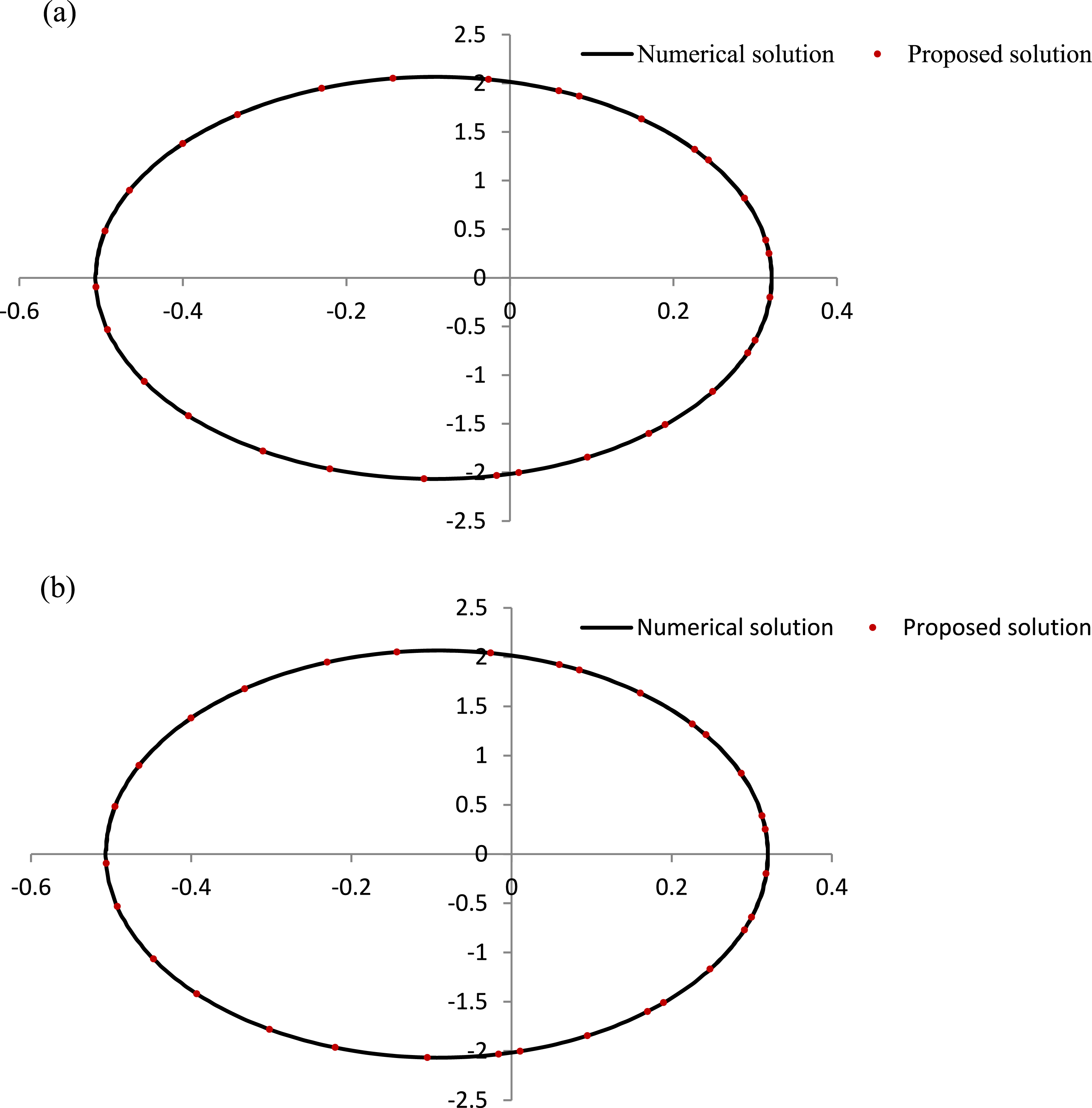
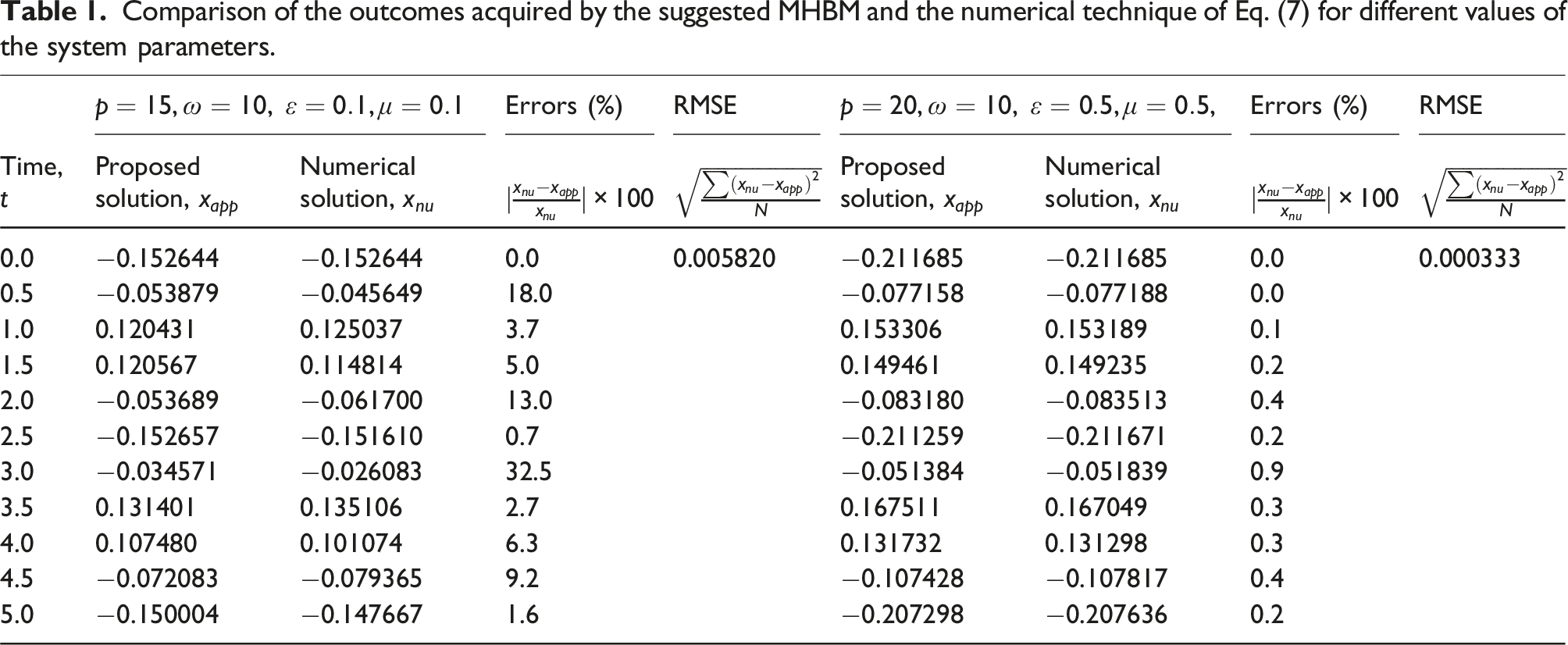
The outcomes have been assimilated with the numerical results for justifying the validity of proposed MHBM. Correlations among the results gained by the said process and the numerical findings have been demonstrated in Figures Figures 1(a)-3(b) for nonlinear forced vibration problems with quadratic-biquadratic, quadratic and biquadratic nonlinearities, respectively, for the diverse values of the system parameters. A comparison has been shown in Figure 1(f) between MHBM and HBM. Furthermore, the phase trajectories have been plotted for various values of the parameters in Figures 4(a)-6(b). Figures have been plotted for different values of the system parameters to justify the validity of the proposed method. Also, comparisons have been shown in tables with numerical errors and root mean square errors (RMSEs). The numerical errors and RMSEs tend to zero. It is also noticed that the errors obtained for the proposed method are less than the errors obtained in HBM. The proposed method performs better than the classical HBM. From the Table 1, it is cear that the accuracy of the proposed method is highly accepted (Table 1).

Figure 1.

(a) Comparison of the time-displacement results of Eq. (7) acquired by the proposed MHBM and numerical method for $p = 10, ω = 5, μ = 0.1, ε = 0.1$ or $x (0) = - 0.009818, \dot{x} (0) = 0.043332$ . (b) Comparison of the time-displacement results of Eq. (7) acquired by the proposed MHBM and numerical method for $p = 20, ω = 10, μ = 0.1, ε = 0.1$ or $x (0) = - 0.204027, \dot{x} (0) = 0.020387$ . (c) Comparison of the time-displacement results of Eq. (7) acquired by the proposed MHBM and numerical method for $p = 10, ω = 5, μ = 0.1, ε = 1.0$ or $x (0) = - 0.523685, \dot{x} (0) = 0.041923$ . (d) Comparison of the time-displacement results of Eq. (7) acquired by the proposed MHBM and numerical method for $p = 10, ω = 5, μ = 0.5, ε = 0.1$ or $x (0) = - 0.425380, \dot{x} (0) = 0.436121$ . (e) Comparison of the time-displacement results of Eq. (7) acquired by the HBM and numerical method for $p = 15, ω = 10, μ = 0.1, ε = 0.1$ or $x (0) = - 0.152558, \dot{x} (0) = 0.015281$ . (f) Comparison of the time-displacement results of Eq. (7) acquired by the proposed MHBM, HBM and numerical method for $p = 10, ω = 5, μ = 0.1, ε = 1.0$ or $x = - 0.523685, \dot{x} (0) = 0.041923$ . (g) Comparison of the time-displacement results of Eq. (7) acquired by the proposed MHBM, HBM and numerical method for $p = 10, ω = 5, μ = 0.1, ε = 1.3$ or, $x (0) = - 0.569034, \dot{x} (0) = 0.040878$ . (h) Comparison of the time-displacement results of Eq. (7) acquired by the proposed MHBM, HBM and numerical method for $p = 40, ω = 10, μ = 0.1, ε = 0.1$ or $x (0) = - 0.413139, \dot{x} (0) = 0.040796 .$ (i) Comparison of the time-displacement results of Eq. (7) acquired by the proposed MHBM, HBM and numerical method for $p = 10, ω = 5, μ = 4.0, ε = 1.0$ or $x (0) = - 0.315739, \dot{x} (0) = 0.935866 .$

Figure 2.

(a) Comparison of the time-displacement results of Eq. (15) acquired by the proposed MHBM and numerical method for $p = 10, ω = 5, μ = 0.1, ε = 0.1$ or $x (0) = - 0.425051, \dot{x} (0) = 0.043341$ . (b) Comparison of the time-displacement results of Eq. (15) acquired by the proposed MHBM and numerical method for $p = 5, ω = 3, μ = 0.1, ε = 0.5$ or $x (0) = - 0.720169, \dot{x} = 0.068322$ or $x (0) = - 1.568814, \dot{x} (0) = 0.062707$ .

Figure 3.

(a) Comparison of the time-displacement results of Eq. (21) acquired by the proposed MHBM and numerical method for $p = 10, ω = 3, μ = 0.1, ε = 1.0$ or $x (0) = - 1.568814, \dot{x} (0) = 0.062707$ . (b) Comparison of the time-displacement results of Eq. (21) acquired by the proposed MHBM and numerical method for $p = 5, ω = 3, μ = 0.1, ε = 0.5$ or $x (0) = - 0.650541, \dot{x} (0) = 0.069438$ .

Figure 4.

(a) Comparison of the phase diagram determined by the proposed method and a numerical method for Eq. (7) when $p = 10, ω = 5, μ = 0.1, ε = 1.0$ or $x (0) = - 0.523685, \dot{x} (0) = 0.041923$ . (b) Comparison of the phase diagram determined by the proposed method and a numerical method for Eq. (7) when $p = 10, ω = 5, μ = 0.1, ε = 0.1$ or $x (0) = - 0.009818, \dot{x} (0) = 0.043332$ .

Figure 5.

(a) Comparison of the phase diagram determined by the proposed method and a numerical method for Eq. (15) when $p = 5, ω = 3, μ = 0.1, ε = 0.5$ or $x (0) = - 0.720169,$ $\dot{x} (0) = 0.068322 .$ (b) Comparison of the phase diagram determined by the proposed method and a numerical method for Eq. (15) when $p = 3, ω = 5, μ = 0.1, ε = 1.0$ or $x (0) = - 0.132646,$ $\dot{x} (0) = 0.012965$ .

Figure 6.

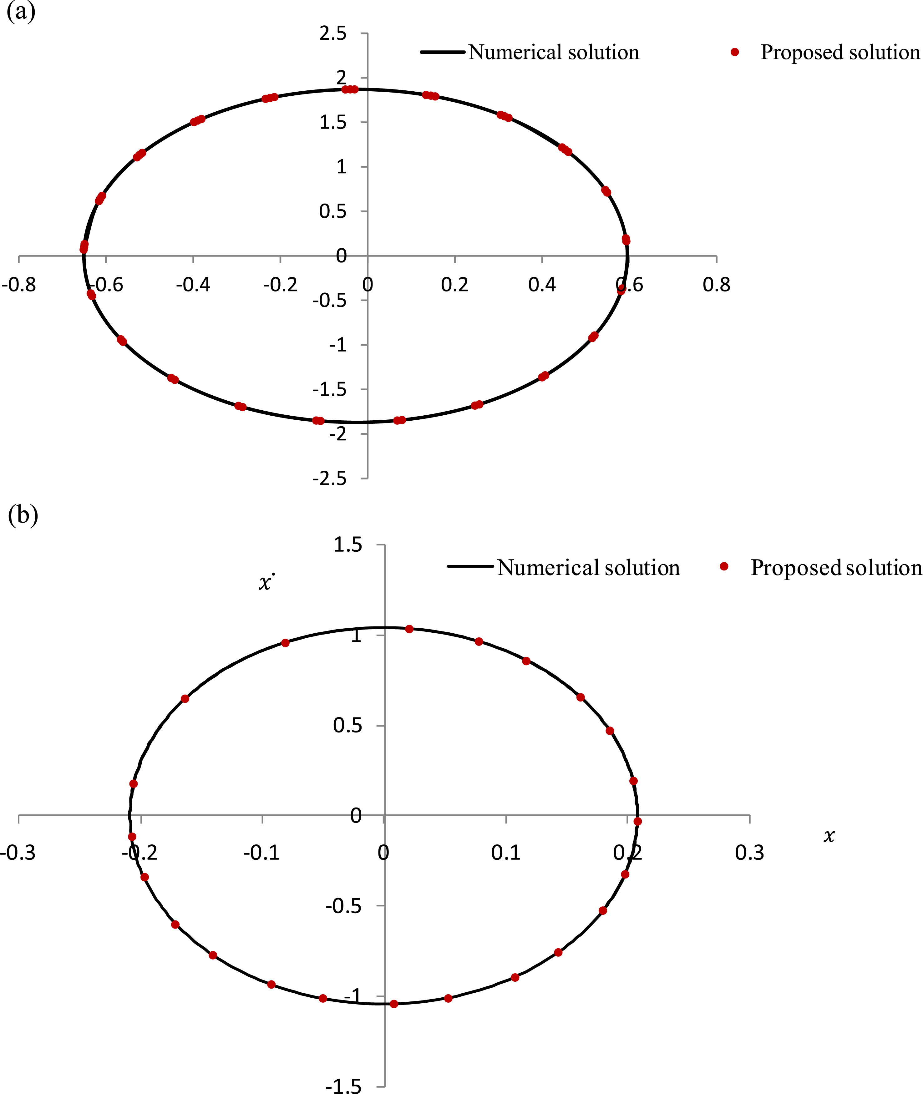
(a) Comparison of the phase diagram determined by the proposed method and a numerical method for Eq. (21) when $p = 5, ω = 3, μ = 0.1, ε = 0.5$ or $x (0) = - 0.0650541, \dot{x} (0) = 0.069438$ . (b) Comparison of the phase diagram determined by the proposed method and a numerical method for Eq. (22a)-(22e) when $p = 5, ω = 5, μ = 0.1, ε = 0.5$ or, $x (0) = - 0.206721, \dot{x} (0) = 0.021305 .$

Table 1.

Comparison of the outcomes acquired by the suggested MHBM and the numerical technique of Eq. (7) for different values of the system parameters.

	$p = 15, ω = 10,$ $ε = 0.1, μ = 0.1$		Errors (%)	RMSE	$p = 20, ω = 10,$ $ε = 0.5, μ = 0.5,$		Errors (%)	RMSE
Time, $t$	Proposed solution, $x_{a p p}$	Numerical solution, $x_{n u}$	$\| \frac{x_{n u} - x_{a p p}}{x_{n u}} \| \times 100$	$\sqrt{\frac{\sum {(x_{n u} - x_{a p p})}^{2}}{N}}$	Proposed solution, $x_{a p p}$	Numerical solution, $x_{n u}$	$\| \frac{x_{n u} - x_{a p p}}{x_{n u}} \| \times 100$	$\sqrt{\frac{\sum {(x_{n u} - x_{a p p})}^{2}}{N}}$
0.0	−0.152644	−0.152644	0.0	0.005820	−0.211685	−0.211685	0.0	0.000333
0.5	−0.053879	−0.045649	18.0		−0.077158	−0.077188	0.0
1.0	0.120431	0.125037	3.7		0.153306	0.153189	0.1
1.5	0.120567	0.114814	5.0		0.149461	0.149235	0.2
2.0	−0.053689	−0.061700	13.0		−0.083180	−0.083513	0.4
2.5	−0.152657	−0.151610	0.7		−0.211259	−0.211671	0.2
3.0	−0.034571	−0.026083	32.5		−0.051384	−0.051839	0.9
3.5	0.131401	0.135106	2.7		0.167511	0.167049	0.3
4.0	0.107480	0.101074	6.3		0.131732	0.131298	0.3
4.5	−0.072083	−0.079365	9.2		−0.107428	−0.107817	0.4
5.0	−0.150004	−0.147667	1.6		−0.207298	−0.207636	0.2

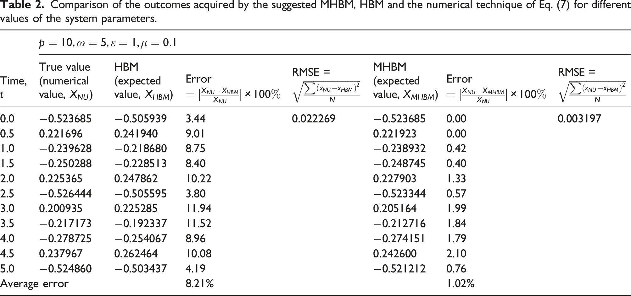
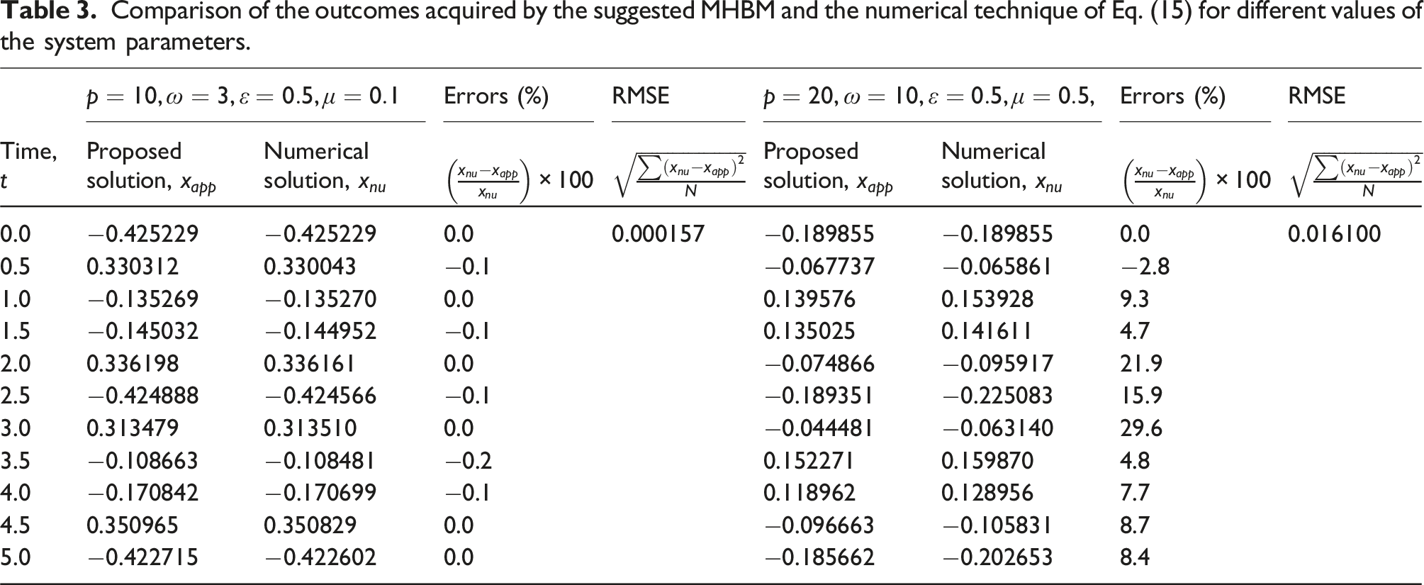
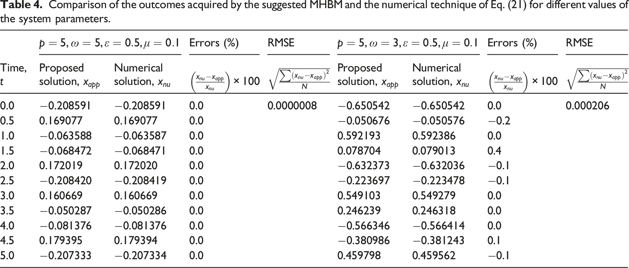
The low errors highlight that the MHBM achieves comparable accuracy with less computational effort compared to HBM (Table 2). Numerical methods are relatively simple but it requires accurate initial numerical guess values and large computational effort to obtain the desired solutions. Also, it does not provide the overall behavior of the nonlinear physical systems. Graphical presentation is important to identify the system’s behavior for any physical problem. To overcome those limitations of the numerical techniques and to obtain the accurate behavior of the physical systems, a MHBM is presented for solving nonlinear damped forced oscillators containing quadratic-biquadratic, quadratic, biquadratic nonlinearities in presence of various damping effects for both strong (

ε = 1.0

) and weak (

ε < 1

) nonlinearities. From the figures, phase diagrams and tables, it is noticed that the results acquired by the MHBM nicely coincide to the results obtained by fourth order Runge-Kutta. The MHBM reformulates the system of nonlinear algebraic equations into a simplified framework involving only a single nonlinear equation. The proposed approach significantly simplifies the computational process by reducing the complexity of the system of equations. In the classical HBM, all simultaneous nonlinear algebraic equations have to be solved numerically and comparisons have been given in Tables 3 and 4 for different values of the system parameters of Eqs. (15) and (22) respectively. It is a difficult task. Numerical resolution of these equations is computationally intensive and time-consuming. The difficulty increases with the complexity of the system, as the convergence of numerical solutions may not always be straightforward. The amplitude describes the system’s energy or maximum displacement during oscillations. The phase provides information about the timing or position of the oscillation within its cycle. Together, amplitude and phase variables offer a comprehensive description of the system’s oscillatory processes. Stability is examined using variational equations derived for amplitude and phase variables. This method of stability analysis is versatile and can be applied to any physical problem involving nonlinear dynamical systems. It enables researchers to predict the system’s response under varying conditions, ensuring robust design and control in practical applications. Graphical representations, such as phase planes or time evolution plots of amplitude and phase are used to detect steady-state solutions, their stability, illustrate transient and long-term behaviors of the system. These visual tools provide insights into whether a system returns to equilibrium or diverges from it under perturbations. This method provides good results for the values for

0 < ε \leq 1

and the analytical solutions converge to the numerical solutions. It is noticed that the proposed method is not suitable for large values of damping

μ

, initial amplitude

p

, forcing frequency

ω

and

ε

(i . e ., ε ≫ 1) .

Also the analytical solutions deviate from the numerical solutions for large values of the initial amplitude of the external force and large damping (please see Figure 1(g)- 1(h)).

Table 2.

Comparison of the outcomes acquired by the suggested MHBM, HBM and the numerical technique of Eq. (7) for different values of the system parameters.

	$p = 10, ω = 5, ε = 1, μ = 0.1$
Time, $t$	True value (numerical value, $X_{N U}$ )	HBM (expected value, $X_{H B M}$ )	Error $= \| \frac{X_{N U} - X_{H B M}}{X_{N U}} \| \times 100 %$	RMSE = $\sqrt{\frac{\sum {(x_{N U} - x_{H B M})}^{2}}{N}}$	MHBM (expected value, $X_{M H B M}$ )	Error $= \| \frac{X_{N U} - X_{M H B M}}{X_{N U}} \| \times 100 %$	RMSE = $\sqrt{\frac{\sum {(x_{N U} - x_{H B M})}^{2}}{N}}$
0.0	−0.523685	−0.505939	3.44	0.022269	−0.523685	0.00	0.003197
0.5	0.221696	0.241940	9.01		0.221923	0.00
1.0	−0.239628	−0.218680	8.75		−0.238932	0.42
1.5	−0.250288	−0.228513	8.40		−0.248745	0.40
2.0	0.225365	0.247862	10.22		0.227903	1.33
2.5	−0.526444	−0.505595	3.80		−0.523344	0.57
3.0	0.200935	0.225285	11.94		0.205164	1.99
3.5	−0.217173	−0.192337	11.52		−0.212716	1.84
4.0	−0.278725	−0.254067	8.96		−0.274151	1.79
4.5	0.237967	0.262464	10.08		0.242600	2.10
5.0	−0.524860	−0.503437	4.19		−0.521212	0.76
Average error			8.21%			1.02%

Table 3.

Comparison of the outcomes acquired by the suggested MHBM and the numerical technique of Eq. (15) for different values of the system parameters.

	$p = 10, ω = 3, ε = 0.5, μ = 0.1$		Errors (%)	RMSE	$p = 20, ω = 10, ε = 0.5, μ = 0.5,$		Errors (%)	RMSE
Time, $t$	Proposed solution, $x_{a p p}$	Numerical solution, $x_{n u}$	$(\frac{x_{n u} - x_{a p p}}{x_{n u}}) \times 100$	$\sqrt{\frac{\sum {(x_{n u} - x_{a p p})}^{2}}{N}}$	Proposed solution, $x_{a p p}$	Numerical solution, $x_{n u}$	$(\frac{x_{n u} - x_{a p p}}{x_{n u}}) \times 100$	$\sqrt{\frac{\sum {(x_{n u} - x_{a p p})}^{2}}{N}}$
0.0	−0.425229	−0.425229	0.0	0.000157	−0.189855	−0.189855	0.0	0.016100
0.5	0.330312	0.330043	−0.1		−0.067737	−0.065861	−2.8
1.0	−0.135269	−0.135270	0.0		0.139576	0.153928	9.3
1.5	−0.145032	−0.144952	−0.1		0.135025	0.141611	4.7
2.0	0.336198	0.336161	0.0		−0.074866	−0.095917	21.9
2.5	−0.424888	−0.424566	−0.1		−0.189351	−0.225083	15.9
3.0	0.313479	0.313510	0.0		−0.044481	−0.063140	29.6
3.5	−0.108663	−0.108481	−0.2		0.152271	0.159870	4.8
4.0	−0.170842	−0.170699	−0.1		0.118962	0.128956	7.7
4.5	0.350965	0.350829	0.0		−0.096663	−0.105831	8.7
5.0	−0.422715	−0.422602	0.0		−0.185662	−0.202653	8.4

Table 4.

Comparison of the outcomes acquired by the suggested MHBM and the numerical technique of Eq. (21) for different values of the system parameters.

	$p = 5, ω = 5, ε = 0.5, μ = 0.1$		Errors (%)	RMSE	$p = 5, ω = 3, ε = 0.5, μ = 0.1$		Errors (%)	RMSE
Time, $t$	Proposed solution, $x_{a p p}$	Numerical solution, $x_{n u}$	$(\frac{x_{n u} - x_{a p p}}{x_{n u}}) \times 100$	$\sqrt{\frac{\sum {(x_{n u} - x_{a p p})}^{2}}{N}}$	Proposed solution, $x_{a p p}$	Numerical solution, $x_{n u}$	$(\frac{x_{n u} - x_{a p p}}{x_{n u}}) \times 100$	$\sqrt{\frac{\sum {(x_{n u} - x_{a p p})}^{2}}{N}}$
0.0	−0.208591	−0.208591	0.0	0.0000008	−0.650542	−0.650542	0.0	0.000206
0.5	0.169077	0.169077	0.0		−0.050676	−0.050576	−0.2
1.0	−0.063588	−0.063587	0.0		0.592193	0.592386	0.0
1.5	−0.068472	−0.068471	0.0		0.078704	0.079013	0.4
2.0	0.172019	0.172020	0.0		−0.632373	−0.632036	−0.1
2.5	−0.208420	−0.208419	0.0		−0.223697	−0.223478	−0.1
3.0	0.160669	0.160669	0.0		0.549103	0.549279	0.0
3.5	−0.050287	−0.050286	0.0		0.246239	0.246318	0.0
4.0	−0.081376	−0.081376	0.0		−0.566346	−0.566414	0.0
4.5	0.179395	0.179394	0.0		−0.380986	−0.381243	0.1
5.0	−0.207333	−0.207334	0.0		0.459798	0.459562	−0.1

Conclusion

The validity of the proposed method is assured through the comparison of the obtained results with the numerical results in the whole solution domain for the different significant values of the systems parameters. The proposed approach significantly simplifies the computational process by reducing the complexity of the system of equations. The results obtained through this process exhibit significant resemblance to the numerical findings presented in the figures, phase planes, and tables. This procedure plays a crucial role in handling strongly as well as weakly nonlinear damped forced dynamical systems with generalized quadratic-biquadratic, quadratic, and biquadratic nonlinearities, respectively, where a truncated Fourier series is chosen as the solution of the differential equations. The proposed technique reduces the large computational effort and requires small computational time than that of other existing harmonic balance methods. It is noticed that the proposed method is suitable for significant values of the system parameters.

Footnotes

Acknowledgments

The author(s) expressed their gratitude to the unknown reviewers for assisting and recognizing the improvements made to the manuscript during the review process. We appreciate their time and effort in raising the concerns, comments, and suggestions to improve the manuscript.

Authors’ Contributions

All authors contributed equally to this study and approved the final manuscript.

Declaration of conflicting interests

The author(s) declared no potential conflicts of interest with respect to the research, authorship, and/or publication of this article.

Funding

The author(s) received no financial support for the research, authorship, and/or publication of this article.

ORCID iD

M Alhaz Uddin

Appendix

References

Wickert

. Non-linear vibration of a traveling tensioned beam. Int J Non Lin Mech 1992; 27: 503–517.

Nayfeh

. Introduction to perturbation techniques. John Wylie, 1993.

Nayfeh

. Perturbation method. New York: John Wiley & Sons, 1983.

Nayfeh

Mook

. Nonlinear oscillations. New York: John Wiley & Sons, 1989.

Krylov

Bogolyubov

. Introduction to nonlinear mechanics. Princeton University, 1948.

Bogoliubov

Mitropolskii

. Asymptotic methods in the theory of nonlinear oscillations. New York: Gordan and Breach, 1961.

Alam

. A unified Krylov-Bogoliubov-Mitropolskiimethod for solving nthorder nonlinear systems, J Franklin Inst, 399 (2) (2002) 239-248.

Alam

Azad

MAK

Hoque

. A general Struble’s technique for solving an nth-order weakly non-linear differential system with damping, Int J Non Lin Mech, 41 (2006) 905-918.

Jones

. Remarks on the perturbation process for certain conservative systems. Int J Non Lin Mech 1988; 13: 125–128.

10.

Cheung

Chen

Lau

. A modified Lindstedt-Poincare method for certain strongly nonlinear oscillators. Int J Non Lin Mech 1991; 26: 367–378.

11.

Alam

Yeasmin

Ahamed

. Generalization of the modified Lindstedt-Poincare method for solving some strong nonlinear oscillators. Ain Shams Eng J 2019; 10(1): 195–201.

12.

Fooladi

Abaspour

Kimiaeifar

, et al. On the analytical solution of Kirchhoff simplified Model for beam by using of homotopy analysis method. World Appl Sci J 2009; 6: 298–302.

13.

Liao

. The proposed homotopy analysis technique for the solution of nonlinear problems. Shanghai JiaoTong University, 1992. Ph.D. Thesis.

14.

. Homotopy perturbation method for nonlinear oscillators with coordinate dependent mass. Results Phys 2018; 10: 270–271.

15.

Uddin

Sattar

Alam

. An approximate technique for solving strongly nonlinear differential systems with damping effects. Indian J Math 2011; 53(1): 83–98.

16.

Uddin

Alom

Ullah

. An analytical approximate technique for solving a certain type of fourth order strongly nonlinear oscillatory differential system with small damping. Far East J Math Sci 2012; 68(1): 59–82.

17.

Wazwaz

. The variational iteration method: a reliable analytic tool for solving linear and nonlinear wave equations. Comput Math Appl 2008; 54: 926–932.

18.

. Some asymptotic methods for strongly nonlinear equations. Int J Mod Phys B 2006; 20: 1141–1199.

19.

Mickens

. A generalization of the method of harmonic balance. J Sound Vib 1986; 111: 515–518.

20.

Rahman

Haque

Shanta

. Harmonic balance solution of nonlinear differential equation (non-conservative). Journal of Advances in Vibration Engineering 2010; 9(4): 334–346.

21.

Wagner

Lentz

. On the detection of artifacts in harmonic balance solutions of nonlinear oscillators. Applied Mathematical Modeling 2019; 65: 408–414.

22.

. Y. The harmonic balance method for Yao-Cheng oscillator. J Low Freq Noise Vib Act Control 2019; 38: 1816–1818.

23.

Yeasmin

Sharif

Rahman

, et al. Analytical technique for solving the quadratic nonlinear oscillator, Results Phys 2020; 18: 103303.

24.

Rahman

Lee

. New modified multi-level residue harmonic balance method for solving nonlinearly vibrating double-beam problem. J Sound Vib 2018; 406: 295–327.

25.

Rahman

Hasan

ASMZ

Yeasmin

. Modified multi-level residue harmonic balance method for solving nonlinear vibration problem of beam resting on nonlinear elastic foundation. Journal of Applied and Computational Mechanics 2019; 5(4): 628–638.

26.

Hasan

ASMZ

Rahman

Lee

, et al. Multi-level residue harmonic balance solution for the nonlinear natural frequency of axially loaded beams with an internal hinge. Mech Adv Mater Struct 2018; 24(13): 1074–1085.

27.

Lee

. Analytic solution for nonlinear multimode beam vibration using a modified harmonic balance approach and Vieta’s substitution, Shock Vib, 2016: 6 pages.

28.

Ullah

Rahman

Uddin

. A modified harmonic balance method for solving forced vibration problems with strong nonlinearity. J Low Freq Noise Vib Act Control 2021; 40(2): 1096–1104. DOI: 10.1188/1461338420923333.

29.

Ullah

Uddin

Rahman

. A modified harmonic balance method for solving strongly generalized nonlinear damped forced vibration systems. Nonlinear Dynam Syst Theor 2021; 21(5): 544–552.

30.

Ullah

Uddin

Rahman

. An analytical technique for handling forced Van der Pol vibration equation. J Bangladesh Acad Sci 2021; 45(2): 231–240.

31.

Ullah

Rahman

Uddin

. Free vibration analysis of nonlinear axially loaded beams using a modified harmonic balance method. Partial Differential Equations in Applied Mathematics 2022; 6: 100414.

32.

Ullah

Uddin

Rahman

. Analytical solution of modified forced Van der Pol vibration equation using modified harmonic balance method, Khulna University Studies. Khulna Univ Stud 2022: 892–903. DOI: 10.53808/KUS.2022.ICSTEM4IR.0180-se.

33.

Kandil

Hamed

Awrejcewicz

. Harmonic balance method to analyze the steady-state response of a controlled mass-damper-spring model. Symmetry 2022; 14: 1247. DOI: 10.3390/sym1406124.

34.

Uddin

Sattar

. An approximate technique for solving strongly nonlinear biological systems with small damping effects. J. of the Calcutta Mathematical Society 2011; 7(1): 51–62.

Nonlinear damped forced oscillators with quadratic-biquadratic nonlinearities

Abstract

Keywords

Introduction

The method

Example

Example

Example

Results and discussion

Conclusion

Footnotes

Acknowledgments

Authors’ Contributions

Declaration of conflicting interests

Funding

ORCID iD

Appendix

References